Comparison of Baseline Load Forecasting Methodologies for Active and Reactive Power Demand

Abstract

Forecasting the electricity consumption is an essential activity to keep the grid stable and avoid problems in the devices connected to the grid. Equaling consumption to electricity production is crucial in the electricity market. The grids worldwide use different methodologies to predict the demand, in order to keep the grid stable, but is there any difference between making a short time prediction of active power and reactive power into the grid? The current paper analyzes the most usual forecasting algorithms used in the electrical grids: ‘X of Y’, weighted average, comparable day, and regression. The subjects of the study were 36 different buildings in Terni, Italy. The data supplied for Terni buildings was split into active and reactive power demand to the grid. The presented approach gives the possibility to apply the forecasting algorithm in order to predict the active and reactive power and then compare the discrepancy (error) associated with forecasting methodologies. In this paper, we compare the forecasting methodologies using MAPE and CVRMSE. All the algorithms show clear differences between the reactive and active power baseline accuracy. ‘Addition X of Y middle’ and ‘Addition Weighted average’ better follow the pattern of the reactive power demand (the prediction CVRMSE error is between 12.56% and 13.19%) while ‘Multiplication X of Y high’ and ‘Multiplication X of Y middle’ better predict the active power demand (the prediction CVRMSE error is between 12.90% and 15.08%).

1. Introduction

The rise in the quantity and diversity of electronic devices makes linking active and reactive power demand harder for every customer [1]. For such a reason, separate active and reactive power forecasting is a viable option. Every electrical grid uses a different approach to predict the electrical consumption. This paper will present popular algorithms used at present, and compare their accuracy, while at the same time showing the contrast between the active power and reactive power forecasting. Hence, we try to contribute to the scientific knowledge of efficient grid management, improving the prediction capacity of reactive power in the grid which facilitates exploitation of Distributed Energy Resources (DER) and integration of the renewable energy sources (RES) into the grid [2].

Forecasting methodologies are based on information from a single variable; that is, forecasting does not need standard deviation calculations that indicate the importance of each variable (weight) in the objective function, as is the case with regression methods, parameter estimation, or data reconciliation [3]. As such, consistency in calculation of the errors can be very important for comparing various algorithms [4] because it works like an indicator that is measured consistently. Additionally, coupling this with some sort of robust filtering like Hampel’s X84 rule [5,6].

The basic algorithm used in the electrical grids to generate Customer Baseline Load (CBL) is ‘X of Y’ methodology, used by, e.g., PJM ISO [7] or CAISO [8], New England ISO (ISONE) employs weighted average to forecasting [9], whereas comparable day and regression are used for short-term power forecasting of wind farms [10,11].

Numerous studies try to improve the baseline accuracy through innovative ideas, different methods, approaches, and assumptions to generate CBL [12].

Table 1. Overview of relevant CBL prediction errors in literature.

Reference	Description	Error
[13]	The authors completed short term forecasting, for 10 industrial customers in Korea.	MAPE 2.8–26%
[1]	The authors examined daily electricity consumption of an administration building located at the Southwark campus of London South Bank University in London.	RMSE 34%
[14]	The authors undertook short term forecasting for eight users and implemented the baselines in a demand response program.	Average real error 1.15–43%
[15]	The authors completed short time load forecasting in buildings blocks situated in California.	MAPE 10.88–17.97%
[11]	The authors simulated 195 scenarios of a non-residential building.	MAPE 22–40%
[16]	The data used in this paper were collected from 162 industrial and commercial customers.	Overall Performance Index 6–23.8%
[17]	The data used in this paper were collected from three commercial buildings in EEUU.	CVRMSE < 20%

shows some of the relevant previous studies with obtained prediction errors.

While several studies presented in Table 1 used Mean Absolute Percentage Error (MAPE) to estimate the CBL predication error, some experts do not recommend using MAPE [18]. According to the International Performance Measurement and Verification Protocol (IPMVP), the best indicator for a proper baseline error estimation is Coefficient of Variation Root Mean Square Error (CVRMSE) with an established threshold for a successful baseline as CVRMSE < 20% when considering hourly energy use [19].

In addition to the studies listed in Table 1, projects using Artificial Neural Networks (ANN) resulted in more accurate forecasting, but strongly were dependent upon the type of buildings and inputted data quality [20]. We also did not apply Support Vector Regression (SVR) because the method to measure the error in this method is not consistent (the training error and the error of when performing the data validation are different in SVR [21]) with the other methods studied in this document, which would not give us the possibility of comparing SVR with the other methods shown [22].

2. Materials and Methods

This research examined electricity demand in 36 buildings situated in Terni (Italy) during the years 2016, 2017, and 2018. The data were collected by the local Distribution System Operator (DSO) ASM Terni S.p.A.; data were gathered by means of Advanced Metering Infrastructure (AMI) installed at the customers’ locations. With respect to the dataset analyzed in this paper, DSO was identified a group of customers for which data were collected every 15 min; it is worth noting that the Italian Authority prescribes to collect only a monthly aggregated measure.

The implemented procedure used the consumption over the previous days to predict the electricity demand in a window event of 30 min. The algorithms used to generate the baselines were based on the most popular statistical methods implemented in the actual electricity market worldwide: ‘X of Y days’, comparable day, weighted average, regression, and comparable day with addition or multiplication adjustments [23]. In order to analyze the data, a ‘Matlab’ script was developed. The script reads the data in ‘.xlsx’ format, generates the baselines for active and reactive power demand, and calculates the errors between the baseline and actual consumption. Mean Absolute Percentage Error (MAPE) [23] and Coefficient of Variation of the Root Mean Square Error (CVRMSE) [24] were calculated.

The baselines can be generated half an hour in advance, or one day in advance of the desired time window.

Table 2. Inputs and outputs of baseline methodologies.

Type	Input	Output
X of Y	Load demand historical	Baseline with one week to one day in advance
Weighted average	Load demand historical	Baseline with one week to one day in advance
Comparable day	Load demand historical	Baseline with one week to one day in advance
Regression	Load demand historical Temperature historical Measurement of temperature	Baseline with one step (half hour) in advance
Adjustments	Load demand historical Measurement of load demand	Baseline with one step (half hour) in advance

shows the inputs and outputs of the applied baseline generation methods. In some cases, the input is a previously generated baseline.

2.1. X of Y

‘X of Y’ is a statistical methodology which uses ‘X’ of the ‘Y’ days before an event. Two alternative approaches are possible: ‘X of Y middle’ and ‘X of Y high’. In the former, ‘X’ takes the middle values of the ‘Y’ quantities, while the latter excludes the lowest (Y-X) values. Usually, the ‘X of Y middle’ is more accurate while ‘X of Y high’ is a more conservative approach [25].

Equations (1) and (2) show the algorithms used to generate the baselines ‘X of Y middle’ and ‘X of Y high’ [26]. Note that subscript t here denotes timestep during the day. In the case of ‘X of Y middle’, the ‘X’ values will be those closest to the average value of the ‘Y’ values, while in the case of ‘X of Y high’ the ‘X’ values will be those closest to the highest value of the ‘Y’ values.

Equation (1) Baseline X of Y middle [26].

$$b_{\left(t\right)}=\frac{1}{X}{\displaystyle \sum }_{d\in Mid\left(X,Y\right)}^{d=X}{l}_{\left(d,t\right)}$$

(1)

Equation (2) Baseline X of Y high [26].

$$b_{\left(t\right)}=\frac{1}{X}{\displaystyle \sum }_{d\in High\left(X,Y\right)}^{d=X}{l}_{\left(d, t\right)}$$

(2)

‘X of Y’ algorithms are used by Pennsylvania–New Jersey–Maryland interconnection (PJM), California Independent System Operator (CAISO), or New York Independent System Operator (NYISO) [26]. A study recommends that (0.4) ≤ (X/Y) ≤ (0.8) and that no data older than 60 days is used to generate the baseline as the weather change can affect the accuracy of the prediction [27]. For ‘X of Y’ algorithms, the current project took into consideration the demand data over a 5 week long period preceding each date and 0.6 ≤ (X/Y) ≤ 0.8, with Y = 5 and X = 3 or X = 4. Such choice is based upon a study [25] that recommended that the electricity demand data used to generate a baseline should be between 30 and 60 days. We selected 5 weeks (35 days) due to weather conditions, i.e., in order to minimize the impact of the changing seasons on predictions. The same study [25] used both Y = 5 and Y = 10. We chose Y = 5 because the number of previous days we selected (35) is closer to 30 than to 60. In the case when a period of time closer to 60 days would be selected, Y = 10 would be preferred.

2.2. Weighted Average

The weighted average algorithm awards more weight to the days further away from the event. The approach gives greater accuracy when there are many irregularities during the day closest to the event [28]. Equations (3) and (4) are used to generate the weighted average baseline [10].

Equation (3) Weighted average (1) [10].

$$W_{\left(t\right)}=\frac{1}{X-1}{\displaystyle \sum }_{d=1}^{d=n-1}{l}_{\left(d,t\right)}$$

(3)

Equation (4) Weighted average (2) [10].

$$b_{\left(t\right)}= \left(1-\gamma \right)W_{\left(t\right)}+\gamma l_{\left(n,t\right)}$$

(4)

In our study, value for the factor γ was taken as 0.9 according to recommendations [26], while the value of n = 5 was chosen for consistency with the ‘X of Y’ methodologies.

2.3. Comparable Day

The comparable day approach is simpler to apply, because it does not use any equation; the approach consists of generating a baseline with information about a ‘similar day’. While ‘similar’ is usually a subjective term, it can be determined by the weather, or day of the week, for example. The temperature is measured and used to forecast the demand using a previous day with a similar temperature; similarly, measurements of rain or snow fall may be considered [11]. Alternatively, our research took into consideration demand a week before an event to generate a new baseline. For example, to predict the electrical demand on a Monday, the data of the previous Monday were used.

2.4. Simple Regression

Simple regression makes a modification to the baseline (b1) and a more precise baseline (b2) using the temperature and the temperature historical data.

Equation (5) Simple regression.

$${\rho }_{\left(d\right)}=\frac{X{{\displaystyle \sum }}_{i=1}^{d-1}{l}_{\left(i\right)}{T}_{\left(i\right)}-{{\displaystyle \sum }}_{i=1}^{d-1}{l}_{\left(i\right)}{{\displaystyle \sum }}_{i=1}^{d-1}{T}_{\left(i\right)}}{X{{\displaystyle \sum }}_{i=1}^{d-1}{T}_{\left(i\right)}^2-{\left({{\displaystyle \sum }}_{i=1}^{d-1}{T}_{\left(i\right)}\right)}^2}$$

(5)

Equation (6) Simple regression.

$$b_{2\left(t\right)}={\rho }_{\left(d\right)}\left(T_{\left(t\right)}^{*}-T_{\left(t\right)}\right)+b_{1\left(t\right)}$$

(6)

Equation (7) Simple regression.

$$T_{\left(t\right)}=\frac{{{\displaystyle \sum }}_{n=1}^X{T}_{\left(n,t\right)}^{*}}{X}$$

(7)

2.5. Adjustments

Adjustments take a previously generated baseline and make an adjustment in the window before an event (half-hour in our research). Three types of adjustments were used in the current research, multiplication adjustment (Equations (8) and (9)), addition adjustment (Equations (10) and (11)), and linear regression adjustment (Equations (12)–(14)) [16].

2.5.1. Multiplication and Addition Adjustments

The multiplication and addition adjustment have the same concept: take a previously generated baseline and use a factor to reduce the error. In the case of multiplication adjustment, the factor multiplies the baseline, while in the case of addition adjustment the factor adds to or subtracts from the baseline. In our study, after making the adjustments, a subsequent physical analysis was undertaken, and we decided to specify zero baseline if the adjusted baseline took negative values. However, our approach is unable to predict negative demand, e.g., in the case when consumers generate electricity.

Equation (8) Multiplication factor.

$$M_{\left(t\right)}=\frac{{{\displaystyle \sum }}_{i=1}^{t-1}{l}_{r\left(i\right)}}{{{\displaystyle \sum }}_{i=1}^{t-1}{b}_{\left(i\right)}}$$

(8)

Equation (9) Multiplication adjusted Baseline.

$$b_{2\left(t\right)}=M_{\left(t\right)}{b}_{\left(t\right)}$$

(9)

Equation (10) Addition factor.

$$S_{\left(t\right)}=\frac{1}{t-1}{\displaystyle \sum }_{i=1}^{t-1}{l}_{r\left(i\right)}-b_{\left(i\right)}$$

(10)

Equation (11) Addition adjusted baseline.

$$b_{2\left(t\right)}=b_{\left(t\right)}+S_{\left(t\right)}$$

(11)

2.5.2. Linear Regression Adjustment

Linear regression is the most comprehensive method to forecast the demand because it takes into consideration the weather. Regression is used to predict the ‘total consumption’ during the day but is not the best way to predict the consumption in a short event window of half an hour [29]. Equations (6) through (8) are used to generate the regression baseline. The main difference between linear regression and simple regression methods is that simple regression does not use temperature, while linear regression does.

Equation (12) Linear regression factor [16].

$${\rho }_{\left(d,t\right)}=\frac{X{{\displaystyle \sum }}_{d=1}^n{l}_{\left(d,t\right)}{T}_{\left(d,t\right)}-{{\displaystyle \sum }}_{d=1}^n{l}_{\left(d,t\right)}{{\displaystyle \sum }}_{d=1}^n{T}_{\left(d,t\right)}}{X{{\displaystyle \sum }}_{d=1}^n{T}_{\left(d,t\right)}^2-{\left({{\displaystyle \sum }}_{d=1}^n{T}_{\left(d,t\right)}\right)}^2}$$

(12)

Equation (13) Linear regression baseline [16].

$$b_{2\left(t\right)}={\rho }_{\left(d,t\right)}\left(T_{\left(t\right)}^{*}-T_{m\left(d,t\right)}\right)+b_{\left(t\right)}$$

(13)

Equation (14) Average temperature [16].

$$T_{m\left(d,t\right)}=\frac{{{\displaystyle \sum }}_{i=1}^t{T}_{\left(i\right)}}{t}$$

(14)

2.6. Short Term Load Forecasting for Baseline Assessment

The electrical demand depends on numerous factors, e.g., temperature, solar radiation, rainfall, occupancy, etc. In order to compare the different algorithms, the current study calculated two baseline prediction errors: Mean Absolute Percentage Error (MAPE) and Coefficient of Variation Root Mean Square Error (CVRMSE). MAPE is the most widely used method to calculate the error [23], clearly showing the gap between the real and predicted values. However, MAPE exhibits drawbacks if the real value is zero or close to zero. In such cases, CVRMSE can prevent divergences [3]. CVRMSE is harder to calculate but does not have problems with the values close to zero. Equation (13) is used to calculate MAPE, while Equations (14) and (15) are used to calculate CVRMSE.

Equation (15) MAPE error.

$$MAPE=\frac{100}{Nb}{{\displaystyle \sum }}_{t=1}^{Nb}\left|\frac{b_{\left(t\right)}-l_{\left(t\right)}}{l_{\left(t\right)}}\right|$$

(15)

Equation (16) CVRMSE error.

$$CVRMSE=\frac{100}{b_m}\sqrt{{{\displaystyle \sum }}_{t=1}^{Nb}\frac{{\left(b_{\left(t\right)}-l_{\left(t\right)}\right)}^2}{Nb}}$$

(16)

Equation (17) Mean baseline value.

$$bm=\frac{{{\displaystyle \sum }}_{t=1}^{Nb}{b}_{\left(t\right)}}{Nb}$$

(17)

2.7. Assessment Average

Our study analyzed different buildings and numerous methodologies. The results are presented as an average for each methodology following Equation (16) (tb is the number of buildings—normally 36—but in some cases can be less because of missing data to generate some of the baselines).

Equation (18) Average error.

$$Average\text{\_}Error=\frac{1}{tb}{\displaystyle \sum }_{i=1}^{tb}Erro{r}_{\left(i\right)}$$

(18)

An additional parameter considered in this study is the number of buildings in which each method exhibits the best results (with the lowest error). Such parameter is shown in Tables 3–6 in the Min columns, whereas the opposite counts of the buildings reporting the worst performance of a particular method are presented in the Max columns.

2.8. Data Normalization

Data normalization typically treats the development of clean data; in order to do this we used MATLAB. Buildings 9 and 36 did not have any indication of the suitable baseline generation methods, as insufficient data were available to generate baselines for them. Such a result may be due to problems with the meters. In building 32, consumption was zero for a large part of the 3 years resulting in mostly zero baseline. We considered such a case as an exception and omitted the results of building 32 from Table 7. The zero consumption could be due to the specific use of the building, e.g., as a warehouse/storage or holiday home, or due to malfunction of the equipment used to measure the electricity consumption.

3. Results and Discussion

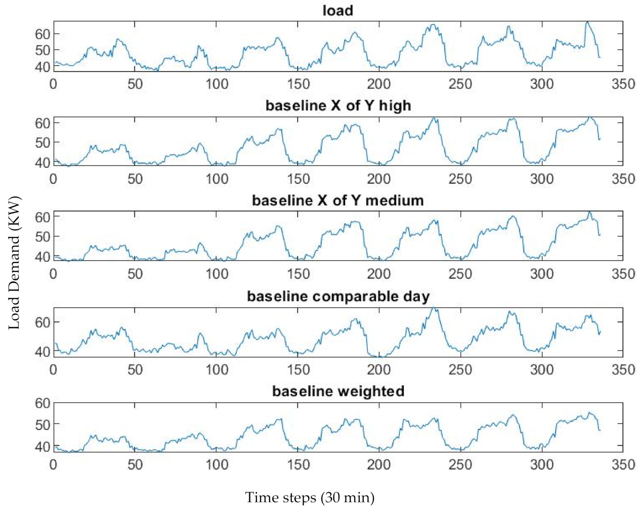
For this study we had 3 years of data, therefore, it was very difficult graphically to see the baseline and the different methods in such a long period of time. For that reason, we included graphs for one week, one graph for active power baselines (Figure 1), and one for reactive power baseline (Figure 2). However, we followed the IPMVP [19] recommendations and used CVRMSE as principal indicator, and we complemented it with MAPE because it is a common indicator and easy to understand.

3.1. Active Power Baseline

Table 3. Baseline, active power, MAPE (highlighted in red are the worst results, highlighted in blue are the best results).

Baseline, Active Power	MAPE [%]			Min			Max
	2016	2017	2018	2016	2017	2018	2016	2017	2018
Normal X of Y high	21.74	25.68	30.45	0	0	0	0	0	0
Normal X of Y middle	20.41	23.61	25.28	0	0	0	0	0	0
Normal comparable day	18.72	18.34	22.43	0	0	1	0	0	0
Normal weighted average	21.56	25.43	30.10	0	0	0	0	0	2
Normal simple regression	27.16	32.54	34.57	0	0	0	12	23	21
Multiplication X of Y high	10.42	9.95	12.97	4	5	6	0	0	0
Multiplication X of Y middle	10.46	9.94	13.44	3	12	8	0	0	0
Multiplication comparable day	11.54	10.93	14.79	5	4	5	0	0	0
Multiplication weighted average	10.48	9.97	13.05	6	6	7	0	0	0
Multiplication simple regression	12.89	12.50	16.14	0	0	1	0	0	0
Addition X of Y high	11.39	10.79	14.40	0	0	0	0	0	0
Addition X of Y middle	10.97	10.15	13.38	3	5	3	0	0	0
Addition comparable day	11.73	11.08	14.43	0	1	2	0	0	0
Addition weighted average	11.22	10.55	14.03	0	0	2	0	0	0
Addition simple regression	13.19	12.17	16.58	0	0	0	0	0	0
Linear regression X of Y high	25.09	26.33	31.04	0	0	0	0	0	0
Linear regression X of Y middle	25.00	26.14	30.71	0	0	0	0	0	0
Linear regression comparable day	25.66	26.80	31.68	0	0	0	2	5	4
Linear regression weighted average	25.04	26.26	30.90	0	0	0	0	0	0
Linear regression simple regression	26.24	27.15	32.17	0	0	0	7	5	7

shows the average MAPE for all buildings. The low error average was obtained for the methodologies with multiplication and addition adjustment. The multiplication adjustment with ‘X of Y high’ has the overall lowest average error over the considered years ranging between 9.95% and 12.97% annually. Baselines generated without adjustment and using linear regression have a similar average error. The simple regression baselines have the highest average error of 34.57% in 2018. Columns ‘Min’ and ‘Max’ in Table 3 show how many buildings have low and high average errors using each of the considered methods. The normal simple regression has the high average error and at the same time is the most common method producing high errors.

The number of minimum and maximum values does not necessarily have to match the number of considered buildings (36), as insufficient electricity demand data for a particular period would prevent baseline generation, meaning that the total number of baselines would be less than 36. Another possibility is that, for the same building, multiple methods might have the same maximum or minimum errors, increasing the number of minimum or maximum counts.

Table 4. Baseline, active power, CVRMSE (highlighted in red are the worst results, highlighted in blue are the best results).

Baseline, Active Power	CVRMSE (%)			Min			Max
	2016	2017	2018	2016	2017	2018	2016	2017	2018
Normal X of Y high	23.29	24.50	45.68	0	0	1	0	0	0
Normal X of Y middle	24.18	25.72	48.48	0	0	0	0	0	2
Normal comparable day	24.67	25.73	50.49	0	0	0	0	0	3
Normal weighted average	24.23	25.55	46.89	0	0	0	0	0	0
Normal simple regression	31.01	32.59	54.16	0	0	0	9	13	13
Multiplication X of Y high	18.96	34.39	43.74	5	3	5	0	1	0
Multiplication X of Y middle	22.57	38.56	44.40	0	1	0	1	1	4
Multiplication comparable day	34.52	39.37	64.16	0	0	0	4	6	8
Multiplication weighted average	19.35	30.36	38.82	0	1	2	0	1	2
Multiplication simple regression	26.78	48.46	53.80	0	0	0	3	7	4
Addition X of Y high	12.59	13.26	26.99	3	6	6	0	0	0
Addition X of Y middle	12.59	13.23	27.00	1	6	10	0	0	0
Addition comparable day	14.05	14.97	30.36	2	6	1	0	0	0
Addition weighted average	12.56	13.19	26.83	8	10	8	0	0	0
Addition simple regression	14.92	15.27	30.80	0	0	1	0	0	0
Linear regression X of Y high	29.41	27.73	46.66	0	0	0	0	0	0
Linear regression X of Y middle	29.44	27.74	46.69	0	0	0	0	0	0
Linear regression comparable day	30.00	28.56	48.04	0	0	0	0	2	2
Linear regression weighted average	29.43	27.72	46.61	0	0	0	0	0	0
Linear regression simple regression	30.39	28.56	48.08	0	0	0	2	2	2

shows the average $\mathrm{CVRMSE}$ for all buildings and the number of buildings with the best and the worst averages for each method. In this case, baseline calculation methods with the highest and the lowest CVRMSE do not match those with the highest number of extreme error values. The lowest CVRMSE is for ‘Addition Weighted average’, ranging between 12.56% and 26.83%, while the same method also has the highest number of buildings with low errors overall during the considered 3-year period.

Depending on the method used to calculate the error, the best baselines are using multiplication setting according to the MAPE calculation or the methods with addition adjustment according to the CVRMSE calculation. Comparatively, MAPE errors were mostly lower than CVRMSE for all prediction methods.

3.2. Reactive Power Baseline

Table 5. Baseline, reactive power, MAPE (highlighted in red are the worst results, highlighted in blue are the best results).

Baseline, Reactive Power	MAPE (%)			Min			Max
	2016	2017	2018	2016	2017	2018	2016	2017	2018
Normal X of Y high	38.01	47.94	48.60	1	1	2	0	0	0
Normal X of Y middle	35.09	50.08	49.39	0	0	2	0	1	0
Normal comparable day	31.90	48.04	46.91	0	0	0	0	1	0
Normal weighted average	38.51	48.55	49.64	0	0	0	2	1	1
Normal simple regression	113.02	109.54	109.84	0	1	0	17	22	25
Multiplication X of Y high	24.83	40.05	39.77	9	8	6	0	0	0
Multiplication X of Y middle	22.42	42.76	43.35	0	2	1	0	4	3
Multiplication comparable day	23.87	43.68	43.63	0	1	0	1	1	0
Multiplication weighted average	25.12	40.26	40.14	2	2	3	1	0	0
Multiplication simple regression	32.06	44.75	47.30	2	4	5	0	0	0
Addition X of Y high	24.65	35.82	35.28	1	2	3	0	0	0
Addition X of Y middle	20.81	35.70	35.19	0	2	6	0	0	0
Addition comparable day	21.79	36.99	36.18	4	2	2	0	0	0
Addition weighted average	24.53	35.56	35.09	1	5	3	1	0	0
Addition simple regression	37.87	51.30	52.56	0	0	0	0	2	3
Linear regression X of Y high	38.35	48.20	44.89	0	2	0	0	0	0
Linear regression X of Y middle	38.57	48.53	44.90	0	0	0	0	0	0
Linear regression comparable day	39.30	49.40	45.83	0	0	1	0	0	0
Linear regression weighted average	38.39	48.23	44.84	0	0	0	0	0	0
Linear regression simple regression	46.54	56.85	54.91	1	0	0	1	1	1

shows the MAPE calculation for the reactive power baselines. The algorithm with the best average error is the ‘Addition X of Y middle’, while ‘Multiplication X of Y high’ has the highest number of buildings with the lowest average errors during the overall 3-year period, despite having approximately 4% higher average error each year.

Table 6. Baseline, reactive power, CVRMSE (highlighted in red are the worst results, highlighted in blue are the best results).

Baseline, Reactive Power	CVRMSE (%)			Min			Max
	2016	2017	2018	2016	2017	2018	2016	2017	2018
Normal X of Y high	27.20	26.69	24.69	0	0	0	0	0	0
Normal X of Y middle	29.49	30.63	28.44	0	0	0	0	0	1
Normal comparable day	28.81	28.99	27.83	0	0	0	0	1	1
Normal weighted average	28.73	28.49	25.89	0	0	0	0	0	0
Normal simple regression	71.04	60.77	60.01	2	5	3	12	11	13
Multiplication X of Y high	31.78	53.17	28.47	1	1	1	1	2	0
Multiplication X of Y middle	50.85	50.54	59.77	0	0	0	1	2	7
Multiplication comparable day	61.48	68.71	64.87	0	0	0	3	7	4
Multiplication weighted average	26.39	57.82	29.72	1	0	1	0	2	0
Multiplication simple regression	23.29	37.39	24.97	0	0	1	0	1	1
Addition X of Y high	15.08	14.52	12.90	5	9	6	0	0	0
Addition X of Y middle	15.36	14.97	13.18	0	2	3	0	0	0
Addition comparable day	16.79	16.06	14.65	2	2	1	0	0	0
Addition weighted average	15.16	14.62	12.90	8	8	10	0	0	0
Addition simple regression	40.89	43.36	39.65	0	0	0	1	1	2
Linear regression X of Y high	32.61	30.77	22.48	0	0	0	0	0	0
Linear regression X of Y middle	32.73	30.92	22.56	0	0	0	0	0	0
Linear regression comparable day	33.22	31.37	23.36	0	0	0	1	0	0
Linear regression weighted average	32.66	30.81	22.47	0	0	0	0	0	0
Linear regression simple regression	49.33	49.87	43.28	0	1	0	0	1	0

shows the CVRMSE calculation where ‘Addition Weighted average’ and ‘Addition X of Y high’ have the same average errors. Baseline calculation methodology with the highest number of buildings with the lowest average error during the overall 3-year period is ‘Addition Weighted average’.

The worst methodology to generate a baseline of reactive power demand is ‘Normal simple regression’ which has the highest average error and the highest number of buildings with high errors (in both cases MAPE and CVRMSE). Comparatively, CVRMSE errors were mostly lower than MAPE for all prediction methods.

3.3. Comparison between Active and Reactive Power Baseline (2016, 2017, and 2018)

Table 7. The most accurate methods used for active (A) and reactive (R) power calculation per building ID.

ID	a	b	c	d	e	f	g	h	i	j	k	l	m	n	o	p	q	r	s	t
1								A				R
2						AR
3												R		A
4						R								A
5						R	A
6									AR
7									AR
8						A				R
9
10												AR
11		R						A
12							A							R
13													A
14	R						A
15							A					R
16							A				R
17							A					R
18						A					R
19									A	R
20												AR	AR
21								A					R
22		R							A
23									AR
24								A						R
25						AR
26			A											R		A
27	R											A
28						R	A
29								A			R
30									A	R
31						AR
32
33							AR
34									A	R
35						A				R
36
A count	0	0	1	0	0	6	8	5	7	0	0	3	2	2	0	1	0	0	0	0
R count	2	2	0	0	0	6	1	0	1	5	3	6	2	3	0	0	0	0	0	0
	Normal
	Multiplication
	Addition
	Linear regression
a	Normal X of Y high
b	Normal X of Y middle
c	Normal comparable day
d	Normal weighted average
e	Normal simple regression
f	Multiplication X of Y high
g	Multiplication X of Y middle
h	Multiplication comparable day
i	Multiplication weighted average
j	Multiplication simple regression
k	Addition X of Y high
l	Addition X of Y middle
m	Addition comparable day
n	Addition weighted average
o	Addition simple regression
p	Linear regression X of Y high
q	Linear regression X of Y middle
r	Linear regression comparable day
s	Linear regression weighted average
t	Linear regression simple regression

shows which algorithm is more accurate for each building. The building ID numbers are presented in the first column, while the other columns correspond to considered baseline generation methods. Each row corresponds to a single building, where A was placed for the baseline calculation method with the lowest MAPE for the active power, and R for the method with the lowest CVRMSE for the reactive power.

In nine buildings, the methods with the lowest error are the same but in the other 25 cases they are not coincident. In only 36% of the cases, we obtained the lowest set by applying a single method to predict active and reactive power; in the rest of the cases it would be better to apply different methods.

4. Conclusions and Future Work

Electrical grids need an upgrade in order to include the innovative technologies of electricity generation (wind turbines, solar panels) and the Distributed Energy Resources (DER). To control a process, it is necessary to understand and predict its main component factors, which in the case of the electrical grid, are the customers and generators. The presented research focuses on prediction of the customers’ characteristics, separating the demand in active and reactive power components for each building to improve the accuracy of demand prediction. The main limitation is the sample profile as all the buildings are located in Terni, Italy, in the Italian electrical market. We recommend that future research should consider other electrical markets subject to different usage patterns. While the used sample of selected buildings provided a representation of building performance, increasing the sample size may allow deeper analysis of singular cases such as the buildings with very rare or occasional electricity consumption.

When talking about active power, MAPE calculation is more important because the active power demand values are usually nonzero. For the reactive power, CVRMSE is more significant, because the reactive power demand can be zero, which makes MAPE calculations inaccurate. Consequently, the lowest error resulted from application of ‘Addition X of Y middle’ and ‘Addition Weighted average’ in prediction of reactive power (the forecasting error is between 12.9% and 15%), while ‘Multiplication X of Y high’ and ‘Multiplication X of Y middle’ provided better prediction of active power demand (the forecasting error is between 9.9% and 12.9%). However, the accuracy of the statistical methods used to generate baselines in this investigation also depended on the building to which they were applied. Better results were obtained by applying different baseline calculation methods to predict the demand for active and reactive power in different years.

Additional research is necessary to verify these findings on a larger customer dataset. In future research, it would be also interesting to investigate the accuracy of prediction methods for active and reactive power in the same building from one day to another, and whether it is better to apply different baseline forecasting methods on specific days. The recommendation would be to take a single building and explore the algorithms studied day by day to see how error varies and whether it is possible to determine which method provides more accurate results on particular days of the week/month/year.

References

- Amber, K.; Aslam, M.; Hussain, S. Electricity consumption forecasting models for administration buildings of the UK higher education sector. Energy Build. 2015, 90, 127–136. [Google Scholar] [CrossRef]
- Jiayi, H.; Chuanwen, J.; Rong, X. A review on distributed energy resources and MicroGrid. Renew. Sustain. Energy Rev. 2008, 12, 2472–2483. [Google Scholar] [CrossRef]
- Di Martino, F.; Loia, V.; Sessa, S. Multi-species PSO and fuzzy systems of Takagi–Sugeno–Kang type. Inf. Sci. 2014, 267, 240–251. [Google Scholar] [CrossRef]
- de Menezes, D.; Prata, D.; Secchi, A.; Pinto, J. A review on robust M-estimators for regression analysis. Comput. Chem. Eng. 2021, 147, 107254. [Google Scholar] [CrossRef]
- Hampel, F.R. The breakdown points of the mean combined with some rejection rules. Technometrics 1985, 27, 95–107. [Google Scholar] [CrossRef]
- Chaudhary, N.; Chowdhury, D.R. Data preprocessing for evaluation of recommendation models in E-commerce. Data 2019, 4, 23. [Google Scholar] [CrossRef] [Green Version]
- Walawalkar, R.; Blumsack, S.; Apt, J.; Fernands, S. An economic welfare analysis of demand response in the PJM electricity market. Energy Policy 2008, 36, 3692–3702. [Google Scholar] [CrossRef]
- Goodin, J. California Independent System Operator demand response & proxy demand resources. In Proceedings of the 2012 IEEE PES Innovative Smart Grid Technologies (ISGT), Washington, DC, USA, 16–20 January 2012; IEEE: Piscataway, NJ, USA, 2012; pp. 1–3. [Google Scholar]
- Ma, F.; Luo, X.; Litvinov, E. Cloud Computing for Power System Simulations at ISO New England—Experiences and Challenges. IEEE Trans. Smart Grid 2016, 7, 2596–2603. [Google Scholar] [CrossRef]
- Yang, X.; Ju, R.; Yuan, Z.; Zhang, Z. Short-term Power Forecasting Method and Application of Wind Farm. MATEC Web Conf. 2018, 232, 04001. [Google Scholar] [CrossRef]
- Ciulla, G.; D’Amico, A. Building energy performance forecasting: A multiple linear regression approach. Appl. Energy 2019, 253, 113500. [Google Scholar] [CrossRef]
- Ruiz, G.R.; Bandera, C.F. Validation of Calibrated Energy Models: Common Errors. Energies 2017, 10, 1587. [Google Scholar] [CrossRef] [Green Version]
- Won, J.-R.; Yoon, Y.-B.; Choi, J.-H.; Yi, K.-K. Case study of customer baseline (CBL) load determination in Korea based on statistical method. In Proceedings of the 2009 Transmission & Distribution Conference & Exposition: Asia and Pacific, Seoul, Korea, 26–30 October 2009; IEEE: Piscataway, NJ, USA, 2010; pp. 1–4. [Google Scholar]
- Escobar, E.; Cadena, A.; Correal, M.E.; Duran, H. Model to calculate the customer base-line for a demand response program in the colombian power market. In Proceedings of the 32nd Annual IAEE Conference “Energy, Economy, Environment: The Global View”, San Francisco, CA, USA, 21–24 June 2009; pp. 1–10. [Google Scholar]
- Zhou, X.; Gao, Y.; Yao, W.; Yu, N. A Robust Segmented Mixed Effect Regression Model for Baseline Electricity Consumption Forecasting. J. Mod. Power Syst. Clean Energy 2020, 1–10. [Google Scholar] [CrossRef]
- Song, T.; Li, Y.; Zhang, X.-P.; Li, J.; Wu, C.; Wu, Q.; Wang, B. A Cluster-Based Baseline Load Calculation Approach for Individual Industrial and Commercial Customer. Energies 2019, 12, 64. [Google Scholar] [CrossRef] [Green Version]
- Effinger, J.; Effinger, M.; Friedman, H. Overcoming barriers to whole building M&V in commercial buildings. In Proceedings of the ACEEE Summer Study on Energy Efficiency in Buildings, Pacific Grove, CA, USA, 12–17 August 2012. [Google Scholar]
- Tofallis, C. A better measure of relative prediction accuracy for model selection and model estimation. J. Oper. Res. Soc. 2015, 66, 1352–1362. [Google Scholar] [CrossRef] [Green Version]
- IPMVP Committee. International Performance Measurement and Verification Protocol: Concepts and Options for Determining Energy and Water Savings, Volume I; (No. DOE/GO-102001-1187; NREL/TP-810-29564); National Renewable Energy Laboratory: Golden, CO, USA, 2001.
- Yang, Y.; Meng, Y.; Xia, Y.; Lu, Y.; Yu, H. An efficient approach for short term load forecasting. In Proceedings of the International Multiconference of Engineers and Computer Scientists, Hong Kong, China, 16–18 March 2011. [Google Scholar]
- Dai, W.; Chuang, Y.-Y.; Lu, C.-J. A Clustering-based Sales Forecasting Scheme Using Support Vector Regression for Computer Server. Procedia Manuf. 2015, 2, 82–86. [Google Scholar] [CrossRef] [Green Version]
- Chen, Y.; Xu, P.; Chu, Y.; Li, W.; Wu, Y.; Ni, L.; Bao, Y.; Wang, K. Short-term electrical load forecasting using the Support Vector Regression (SVR) model to calculate the demand response baseline for office buildings. Appl. Energy 2017, 195, 659–670. [Google Scholar] [CrossRef]
- AleaSoft Energy Forecasting. European Electricity Markets Panorama: Italy. 2018. Available online: https://aleasoft.com/european-electricity-markets-panorama-italy (accessed on 25 July 2019).
- Taylor, J.W. Triple seasonal methods for short-term electricity demand forecasting. Eur. J. Oper. Res. 2010, 204, 139–152. [Google Scholar] [CrossRef] [Green Version]
- EnerNOC Utility Solutions. Energy Baseline Methodologies for Industrial Facilities; Northwest Energy Efficiency Alliance: Portland, OR, USA, 2013. [Google Scholar]
- Mohajeryami, S.; Doostan, M.; Asadinejad, A.; Schwarz, P. Error Analysis of Customer Baseline Load (CBL) Calculation Methods for Residential Customers. IEEE Trans. Ind. Appl. 2016, 53, 5–14. [Google Scholar] [CrossRef]
- Križanič, F.; Oplotnik, Z.J. Analysis of the Energy Market Operator Activity in Eight European Countries. Int. J. Energy Econ. Policy 2014, 4, 716–725. [Google Scholar]
- Lora, A.T.; Santos, J.M.R.; Expósito, A.G.; Ramos, J.L.M.; Santos, J.C.R. Electricity market price forecasting based on weighted nearest neighbors techniques. IEEE Trans. Power Syst. 2007, 22, 1294–1301. [Google Scholar] [CrossRef] [Green Version]
- Tsekouras, G.; Dialynas, E.; Hatziargyriou, N.; Kavatza, S. A non-linear multivariable regression model for midterm energy forecasting of power systems. Electr. Power Syst. Res. 2007, 77, 1560–1568. [Google Scholar] [CrossRef]
Figure 1.
Active power baseline building 3.
Figure 2.
Reactive power baseline building 3.