
Photovoltaic Evaporative Chimney I–V Measurement System
by
 , , , and
Pablo Casado
1, 
José M. Blanes
1 ,
,
Francisco Javier Aguilar Valero
2,
Cristian Torres
1,
Manuel Lucas Miralles
2 and
Javier Ruiz Ramírez
2,* 1
Industrial Electronics Group, Miguel Hernández University of Elche, Avda. de la Universidad, s/n, 03202 Elche, Spain
2
Department of Mechanical Engineering and Energy, Miguel Hernández University of Elche, Avda. de la Universidad, s/n, 03202 Elche, Spain
*
Author to whom correspondence should be addressed.
Energies 2021, 14(24), 8198; https://doi.org/10.3390/en14248198
Submission received: 30 October 2021
/
Revised: 2 December 2021
/
Accepted: 4 December 2021
/
Published: 7 December 2021
(This article belongs to the Special Issue Solar Cooling and Heating Technologies)
Abstract
:The photovoltaic evaporative chimney is a novel solar-cooling system that serves a double purpose: it increases the efficiency of the photovoltaic (PV) panels and it cools down a water stream which can be used to dissipate the heat from a refrigeration cycle. One of the major issues arising from the operation of the chimney is the temperature stratification in the panel due to the movement of the air in the chimney. This effect can trigger the activation of the bypass diodes of the module, creating local maximum power points (MPP) that can compromise the grid-tied inverter tracking. To fill this gap, this paper deals with the design and implementation of an I–V curve measurement system to be used in the performance analysis of the system. The I–V curve tracer consists of a capacitive load controlled by a single board computer. The final design includes protections, capacitor charging/discharging power electronics, remote commands inputs, and current, voltage, irradiance, and temperature sensors.The results show that the modules bypass diodes are not activated during the tests, and no local MPPs appear. Moreover, the curves measured show the benefits of the photovoltaic chimney: the cooling effect increases the power generated by the PV panels by around 10%.
1. Introduction, Background, and Objectives
1.1. Introduction
The 2030 climate and energy framework includes EU-wide targets and policy objectives for the period from 2021 to 2030. It addresses the key actions required across all sectors to allow the EU to move towards a decarbonized economy. The key targets for 2030 include at least 40% cuts in greenhouse gas emissions (from 1990 levels), at least 32% share for renewable energy, and at least 32.5% improvement in energy efficiency.
According to EU information, 40% of the total energy consumption of the Union comes from the buildings sector, and this is responsible for 36% of greenhouse gas emissions. In this sense, the European Directives are focused on improving the energy efficiency of buildings to reach the ambitious goal of carbon neutrality by 2050. The EU has established a legislative framework in order to boost the energy performance of buildings, which includes the Energy Performance of Buildings Directive (EPBD) 2010/31/EU and the Energy Efficiency Directive 2012/27/EU.
The energy consumption in buildings due to space cooling has skyrocketed in the last decades, more than tripling in the last 30 years. It is therefore expected that the energy demand for space cooling and, as a consequence, the energy use to meet that demand, will continue to grow for decades to come [1]. There are several applications in the tertiary sector, such as offices or hospitals, where the thermal demand for heating and cooling matches the sunshine duration. In these cases, the use of solar energy to power air conditioning systems is an attractive idea. This solution could be particularly interesting in places with high solar irradiance and long days.
Solar cooling systems can be classified into two main categories, depending on the type of energy used to drive them: solar thermal cooling systems and solar electric cooling systems. The works of Kim and Ferreira [2] and Ghafoor and Munir [3] include a state-of-the-art review of different solar cooling technologies. In solar thermal cooling systems, solar thermal collectors generate heat that is used to drive a thermal cooling system (usually involving the physical phenomena of sorption). In solar electric cooling systems, PV panels generate electricity which is used to drive the compressor of a heat pump (vapor-compression system). Several studies comparing different solar cooling technologies (PV or thermally driven) in terms of performance can be found in the literature [4,5,6,7,8].
The surveyed literature has shown how difficult is for solar thermal cooling technologies to compete with solar electric cooling systems due to technical and economic reasons. According to Mugnier et al. [9], International Energy Agency Task 53, PV driven compression systems are the most promising and the closest to market solar solution today in the case of small to medium units. Photovoltaic-driven air conditioners will play a major role in reducing the energy consumption in buildings [10]. This alternative becomes even more attractive because of the cost decrease and the increase of the panels’ performance.
In PV panels, the operating temperature plays a key role in the conversion process. It is known that the efficiency of a solar cell decreases with increasing temperature. Typical values for commercially available multicrystalline silicon cells are around 14–19%. That means that the remainder radiated solar energy is transformed into heat, causing the heating of the solar cells.According to Biwole et al. [11], the drop in the efficiency is about 0.5%/°C. This implies that the power production can decrease up to 22% in summer periods (operating temperatures ranging 40–70 °C). Therefore, the temperature regulation of PV modules is important in order to enhance their efficiency, and it can be achieved by either active or passive cooling techniques. Chandrasekar et al. [12] reported a detailed review of thermal regulation techniques for PV modules. Active cooling techniques imply the use of water or air as coolant agent. Significant benefits concerning the PV module performance have been reported [13,14,15,16]. Some disadvantages concern the extra external (cooling media) energy consumption to create the fluid flow and the initial investment. Regarding passive techniques, the application of phase-change materials (PCM) is the most popular solution. Owing to their high heat of fusion, PCM can absorb a lot of energy before undergoing a phase change (melting or solidifying). The PCM temperature remains constant during this phase transition. Therefore, the integration of PCM and PV modules constitutes an attractive alternative to the temperature regulation problem, as the panels remain at a constant temperature when they are integrated with PCM. Another advantage is that the stored heat can be reused for further enhancement of the efficiency of the system (as a PV-T). A detailed study investigating the combination of PV and PCM can be found in [17]. The cyclic stability of the PCM and the poor thermal conductivity constitute the major limitations according to the authors.
1.2. Background: The Photovoltaic Evaporative Chimney
The photovoltaic evaporative chimney is a novel solar electric cooling system. A schematic representation of the system is shown in Figure 1. As it can be seen, it consists of a solar chimney that has been attached to the rear side of a PV panel. A buoyancy-driven flow is induced in the channel of the chimney closer to the module due to the temperature difference between the panel and the ambient air. As a result, this flow cools down the panel, increasing its performance. On the other hand, water is sprayed by a series of nozzles in parallel with the airflow in the other channel of the chimney. As in a cooling tower, a small part of the water evaporates, cooling the remaining water. Depending on the ambient conditions, the air in contact with the water can even be cooled, resulting in a further enhancement of the cooling effect in the panel. Therefore, the system serves a double purpose: increasing the efficiency of the PV panel and cooling down a water stream which can be used to dissipate the heat from a refrigeration cycle (water–water heat pump).
The system was firstly defined and assessed by Lucas et al. [18]. The authors compared two PV modules, one naked (Module 1) and the other operating alongside with an evaporative chimney (Module 2), and they reported an electrical efficiency improvement of 4.9%.
Figure 2 shows the temperature distributions on the PV modules, measured by 18 thermocouples installed in the panels. In this figure, the average temperature of three thermocouples horizontally averaged in each section (bottom, middle, and top of the panels) is depicted.
The temperature levels are fairly constant in Module 1. However, a temperature stratification is observed in Module 2. This effect is produced by the movement and heating of the air inside the chimney. The refrigeration of the panel is quite significant in the bottom section, where the difference of temperatures is higher than 10 °C between the two panels, less evident in the middle (3.5 °C), and almost ineffective in the upper part of the panel (1 °C).
Nowadays, most PV modules use bypass diodes to prevent output current reduction and hot-spots due to shading effects [19]. In a PV module, all the cells connected in series carry the same current. When there is a mismatch in the cells’ working conditions, and some cells produce more current than others, the current flow will find the bypass diode’s path reducing the output voltage. Usually there is not one bypass diode per cell; instead, the cells are grouped in strings and one bypass diode is used in each string. The activation of bypass diodes has one undesired effect, it creates local maximum power points (MPP), and the maximum power points tracking (MPPT) circuit precision can be compromised.
Figure 3 shows the configuration of the solar modules used in the experimental setup presented in Lucas et al. [18], model Sunrise SR-P660255 (Table 1). These solar modules have 60 cells in series divided in three strings of 20 cells; each string has two bypass diodes in parallel.
In the case that one of the strings is not able to generate the same current that the other ones, its respective bypass diode will be activated, and the resulting I–V and P–V curves will have the shape of the curves shown in Figure 4. The situation could be even worse if there is a mismatch between the three strings; in this case, three zones will appear (two diodes activated, one diode activated, and no diode activated, with three different local MPP).
In the literature, these electrical mismatch conditions are usually related with shading, but, if nonuniform artificial cooling is used, cell temperature mismatches could also trigger this effect. Under the same irradiance conditions, cells at lower temperature can produce more power because their open-circuit voltage is higher and so is the MPP voltage, but, on the other hand, their short-circuit current is slightly decreased, so there are some cells that produce more current than others, showing a potential option to activate the bypass diodes.
To date, the experimental tests presented to assess the efficiency of the evaporative chimney have been always performed on a system where the photovoltaic panels are directly connected to a grid-tied inverter. It is supposed that the inverter maximum power tracking (MPPT) system ensures the extraction of the maximum power available, although if local maximums are presented this could not be the case. This fact constituted the main motivation of this work.
1.3. Objectives
To fill this gap, the aim of this work was to design and implement an electronic system to measure the full I–V of the PV modules in real time, in order to ensure that the evaporative cooling system is not producing enough cell temperature mismatching conditions to activate the string bypass diodes, and that the power extracted by the inverter is the maximum.
2. Materials and Methods
2.1. Experimental Facility: The Evaporative Photovoltaic Chimney
The pilot plant where the experiments were conducted (Figure 5) is located in Elche, southeast Spain. It consists of four PV panels (Sunrise model SR-P660255 (see Table 1)) integrated with four evaporative chimneys. The orientation for the PV panels is true south, and they are tilted at an angle of 45°. As previously mentioned, the evaporative system chimney cools the panels down due to the buoyancy-driven flow induced in the convective zone, and rejects the heat from the condenser of a water-cooled chiller in the evaporative area.
A series of sensors were used to measure the performance of the photovoltaic evaporative chimney. Figure 6 depicts the sensors installed in the pilot plant. During the experiments carried out in this investigation, the variables that were monitored and recorded were the solar radiation and the environmental conditions. The experimental facility includes a first-class pyranometer to measure the solar irradiance, while the ambient air temperature, the air relative humidity, the wind speed, and the wind direction were measured with a meteorological station (see Figure 5a). The sensors specifications are shown in Table 2. An Agilent 34972A data-acquisition system was used to monitor and record all the data measured during the experiments. The recording time step was set to 10 s.
2.2. Experimental Procedure
Several sets of experiments were conducted during the summer of 2021. The tests were carried out following the procedure indicated in Ruiz et al. [20]. During the experiments, the I–V curve tracer, described in Section 2.3, was connected to one of the PV panels (panel 4, left-hand side of Figure 5b) in order to measure the performance of the module. During the experimental tests campaign, some experiments were performed with the evaporative chimney attached to panel 4 deactivated (no water flow). The aim was to compare the I–V curves of this panel with the chimney on and off.
2.3. I–V Measurement System Design
To measure PV modules I–V curves, different methods can be used, although their principle of operation is the same. They are based on a controlled sweep of the current provided by the panel, from the short-circuit point to the open-circuit point. The methods described in the literature to perform the curve sweep are as follows:
- (1)
- Variable Resistance. The simplest way to measure the I–V curve is by using a variable resistor connected directly to the panel. The value of the resistor is increased in small steps from zero to open circuit, measuring the current and voltage provided by the panel in each step. These variations can be carried out manually [21], making the process very slow or automated [22,23] (for example connecting different resistors in parallel and using switches controlled by a computer and automating the measurements). This method is only valid for low-power installations, because during the measurement all the generated power by the PV modules are dissipated in the resistors.
- (2)
- Electronic Load. The electronic load method is based on using a transistor as a variable load connected to the panel [24,25,26,27]. To sweep the curve, the transistor works in the three possible modes of operation (on, linear zone, and off), controlled by the voltage applied to the gate. The great advantage of this method, with respect to the variable resistance, is its simpler control and the fast and accurate variation of the transistor equivalent resistance. This method can only be used for medium/low power measurements, as the transistor must be able to dissipate all the power supplied by the photovoltaic installation.
- (3)
- DC–DC Converter. The DC–DC converter’s ability to emulate a resistor has been used in many applications. This ability can also be applied to obtain the I–V curves in PV applications [28]. The value of the emulated resistance can be varied by modifying the converter duty cycle; therefore, if a duty cycle sweep is performed, a characteristic curve sweep will also be performed. Buck–boost-type converters and their variations (SEPIC and Cûk) are the only ones that allow a complete sweep of the curve. Buck-type converters do not allow the curve to be captured near the short-circuit point, and Boost-type ones do not allow capture of the open-circuit point. The main problem with this methodology is the current/voltage ripple caused by the commutations, which makes it difficult to accurately measure the curve.
- (4)
- Capacitive Load. This measurement method is based on connecting the PV modules to a high-capacity discharged capacitor. The capacitor will charge from zero volts up to the module open-circuit voltage of the panel, sweeping the entire characteristic curve [23,29]. The capacitance needed depends on the speed of the measurement equipment, the short-circuit current, and the open-circuit voltage of the modules.
The implemented curve tracer is based on this last method because of its simplicity and accuracy. For the connection and disconnection of the installation to the measurement equipment, a relay with four poles is used while the charging and discharging of the capacitor is controlled by two IGBTs transistors. The capacitor current and voltage during the sweep are captured through an Analog Discovery 2 USB oscilloscope connected to a single-board computer, Raspberry Pi 4 model B, which controls the full process and also acquires the data from the temperature and irradiance sensors that are connected through an analog–digital converter via I2C protocol. The full I–V curve acquisition process was automated with a Python application, and a user-friendly interface was created. Figure 7 shows a simplified block diagram of the I–V curve tracer designed.
2.3.1. Power Electronics Circuit
The main element is the capacitor with a capacitance high enough so the charging process is not excessively fast and allows the acquisition of enough sensed points to characterize the curve. It is worth noting that the distribution of points acquired on the curve is not uniform, as initially (when the capacitor is discharged) the photovoltaic module will provide its maximum current and the capacitor will charge quickly, and at the end of the acquisition, the photovoltaic module approaches its open circuit, providing low current and charging the capacitor slowly. Taking into account that the acquisition system maximum sample rate is 100 MS/s, the capacitor was designed so it can acquire more than one thousand points of the curve in the worst-case scenario (maximum short-circuit current 22 A, minimum open-circuit voltage 10 V), so a 2200 F capacitance is needed. Finally, a 2200 F/3000 V Vishay electrolytic capacitor was selected. The rest of the power circuit consists of a relay that is used to isolate the photovoltaic panel from the system when no measurements are needed. Moreover, the IGBTs transistors have the function of connecting and disconnecting the capacitor to charge it through the module or to discharge it through a resistor.
2.3.2. Measurement Circuit
The data to be measured during each curve capture are the capacitor, voltage and current, the ambient temperature, and the irradiance. For voltage and current measurements, the LV25-P and LA55-P sensors from the LEM manufacturer (Geneva, Switzerland) are used. The outputs of these sensors are directly connected to an Analog Discovery 2 USB oscilloscope that is controlled by the Raspberry Pi 4. The temperature is measured with a Texas Instruments LM35 sensor and the irradiance with a sensor model 6450 from the manufacturer Davis (Hayward, CA, USA). The temperature and irradiance sensors are connected to an analog–digital converter ADS1015 from Adafruit that communicates with the Raspberry Pi using the I2C communication protocol.
2.3.3. Control Circuit
The control circuit is governed by a single-board computer, the Rapsberry Pi 4 model B, which controls the power electronics and the measurements circuits. All control and monitoring software was programmed in Python. A 7” touchscreen is used to program, export, and represent the measurements. The system has also wireless connection so it can be used remotely if a wireless network is available. All the system is powered by a 12 V DC input; this input can be a battery or a commercial AC/DC adapter. Figure 8 shows the I–V curve tracer system; it is not assembled so that the different parts can be shown.
3. Results and Discussion
3.1. I–V Curves
Figure 9 shows two thermographic photographs of the PV module number 4 operating along with an evaporative chimney. Both photographs were taken under the same irradiance and ambient temperature conditions during different days. In Figure 9a, the evaporative chimney is not activated, while in Figure 9b, it is activated. The cooling effect of the evaporative chimney is evident, and so is the temperature stratification with a more than 20 °C difference between the lower and upper part of the PV, matching the results reported by Lucas et al. [18], Figure 2.
To ensure that the temperature stratification caused by the chimney does activate the bypass diodes causing local maximums, regardless of the ambient conditions, a periodic measurement of the curves was programmed, and a curve sweep was performed every one minute. The results are shown in Figure 10. As it can be seen, the temporal evolution of the I–V curves from 10:52 h to 12:19 h in the morning (Figure 10a), for a PV panel operating alongside with the evaporative chimney, does not present local maximums. Figure 10b presents the temporal evolution of the P–V curves. As it can be seen, the power generated by the modules decreases from 200 to 150 W in the period 10–12 h. This can be explained by to the increase in the ambient temperature and the irradiance during the day. While the temperature changed from 20.43 °C to 29.11 °C, the radiation increased from 887 to 1035.7 W/m.
It should be noted that the maximum experimental uncertainty value for the PV power is 10.80%. It was calculated according to the ISO Guide [30] (type B evaluation for standard uncertainty and level of confidence of 95% for the expanded uncertainty), taking into account the accuracy of the developed curve tracer.
3.2. Influence of the Evaporative Chimney on the I–V Curves
Once it was assessed that the evaporative chimney does not activate the bypass diodes, the effect of the chimney on the performance of the panels, via the I–V curves, were analyzed. Figure 11 shows two examples of curves measured with the designed I–V curve tracer. Both curves were measured under same irradiance and ambient temperature conditions (1005 W/m and 21 °C). The difference between both measurements is the solar chimney system activation. It can be seen that, although the PV module temperature is not uniform when the chimney is activated, the bypass diodes of the panel are not activated, and no local maximums appear in the P–V curve. The advantage of using the evaporative chimney is highlighted. As it can be seen in the figure, although the short-circuit current is slightly reduced due to the cooling effect, the open-circuit voltage increases from 32.40 V to 34.49 V. As a result, there is an increase of the maximum power generated by the module. In this example, the maximum power increase was around 11% with the use of the chimney (197 W versus 177 W).
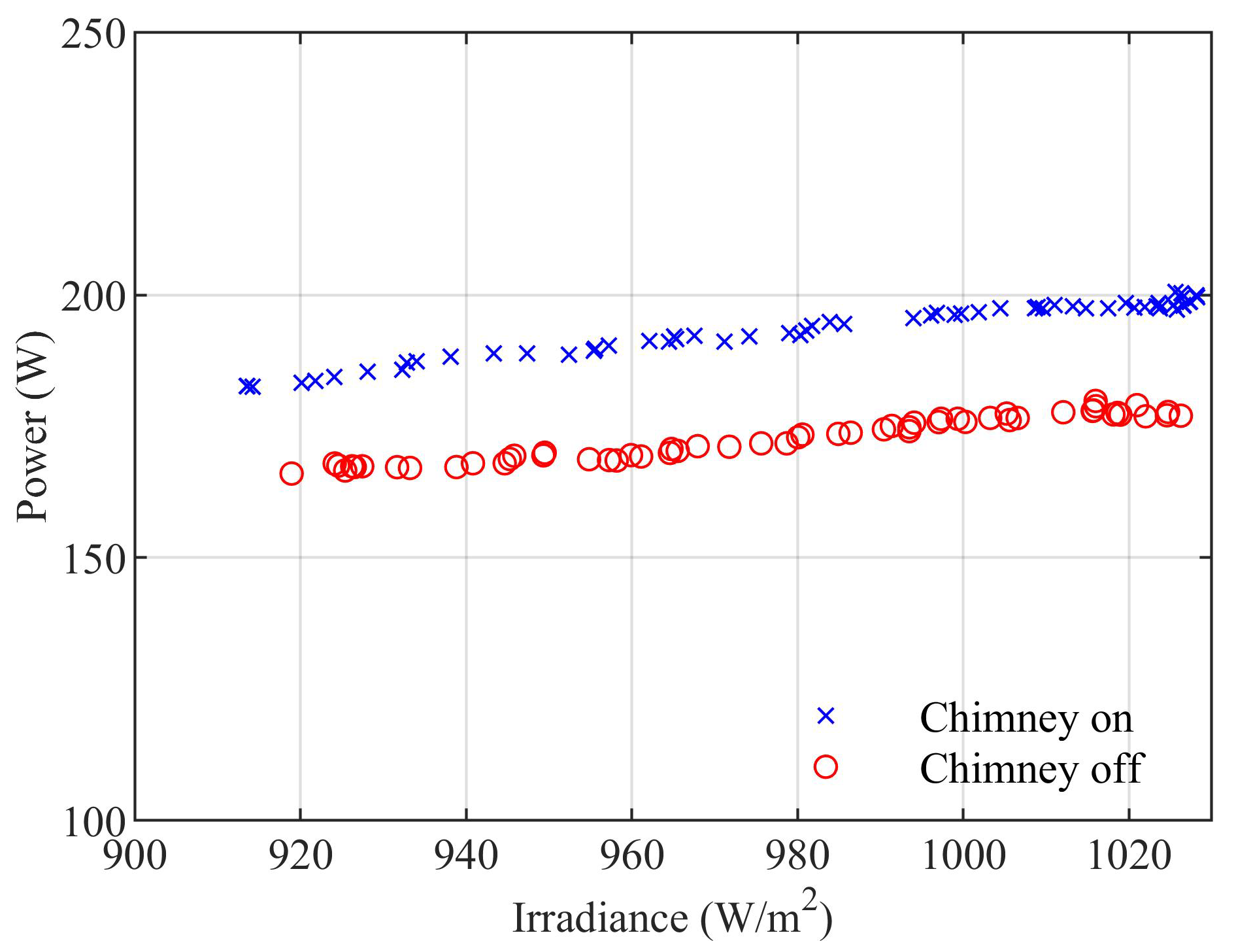
Finally, a comparison between the maximum power extracted with the chimney activated and deactivated for difference irradiance levels is shown in Figure 12. It is worth noting that the tests were performed during two different days, at the same hours, and the ambient temperature was almost the same both days. The whole I–V curve was measured each minute using the designed curve measurement system, and the maximum power was extracted later just for the comparison. The benefits of evaporative chimney cooling effects are obvious, increasing the power extracted from the PV modules at the same working conditions.
4. Conclusions
This study has enabled the investigation of the performance of an evaporative cooling chimney. The main motivation to conduct this work was to investigate if the temperature stratification in the panel due to the air circulation in its rear side activated the bypass diodes of the module, creating local maximum power points (MPPs). To fill this gap, an I–V curve measurement system was developed and implemented, and the full I–V curves were measured in real time. The main findings obtained during this investigation can be summarized as follows:
- The modules bypass diodes are not activated during the experimental tests despite the temperature stratification that appears in the PV modules. Therefore, the MPPT of the grid-tied inverter is not compromised.
- The photovoltaic chimney system improves the efficiency of the panels. For a typical case, the short-circuit current is slightly reduced, while the open-circuit voltage increases from 32.40 V to 34.49 V. As a result, there is an increase of the maximum power generated by the module, typically from 180 W to 200 W (10% increase).
- The power generation slightly increases with the level of solar irradiance for the same ambient temperature. The improvement of power generation remains fairly constant between the cases where the chimney is activated and deactivated.
Future Works
Once it is assessed that the modules bypass diodes are not activated, and no local MPP appear, the I–V curve tracer can be used for different purposes:
- Analyzing the influence of the operating conditions (i.e., water flow rate sprayed by the nozzles, number of chimneys activated, heat load, etc.) on the system performance.
- Implementing other active cooling techniques to achieve the temperature reduction of the panels (i.e., water sliding onto the front surface of the panels (Lucas et al. [31]).
- Conducting a thorough economic analysis of the system, including all the costs and taking into account the integration between the electrical energy demand of the heat pump and the PV energy generation hourly profiles. The study can be extended to different climatic conditions (e.g., Mediterranean climates).
Author Contributions
Conceptualization, P.C., C.T. and J.M.B.; software, P.C., C.T. and J.M.B.; formal analysis, P.C., F.J.A.V. and J.R.R.; investigation, P.C., C.T. and J.R.R.; data curation, P.C., J.M.B. and J.R.R.; writing—original draft preparation, J.M.B., F.J.A.V. and J.R.R.; writing—review and editing, J.M.B., M.L.M. and J.R.R.; supervision, M.L.M. and J.R.R. All authors have read and agreed to the published version of the manuscript.
Funding
This research received no external funding.
Conflicts of Interest
The authors declare no conflict of interest.
Abbreviations
The following abbreviations are used in this manuscript:
| Symbols | |
| I | current (A) |
| P | power (W) |
| V | voltage (V) |
| Abbreviations | |
| PV | photovoltaic |
References
- IEA. The Future of Cooling: Opportunities for Energy-Efficient Air Conditioning; Annual Report; IEA: Paris, France, 2018.
- Kim, D.; Ferreira, C.I. Solar refrigeration options—A state-of-the-art review. Int. J. Refrig. 2008, 31, 3–15. [Google Scholar] [CrossRef]
- Ghafoor, A.; Munir, A. Worldwide overview of solar thermal cooling technologies. Renew. Sustain. Energy Rev. 2015, 43, 763–774. [Google Scholar] [CrossRef]
- Fong, K.; Chow, T.; Lee, C.; Lin, Z.; Chan, L. Comparative study of different solar cooling systems for buildings in subtropical city. Sol. Energy 2010, 84, 227–244. [Google Scholar] [CrossRef]
- Otanicar, T.; Taylor, R.A.; Phelan, P.E. Prospects for solar cooling—An economic and environmental assessment. Sol. Energy 2012, 86, 1287–1299. [Google Scholar] [CrossRef]
- Hartmann, N.; Glueck, C.; Schmidt, F. Solar cooling for small office buildings: Comparison of solar thermal and photovoltaic options for two different European climates. Renew. Energy 2011, 36, 1329–1338. [Google Scholar] [CrossRef]
- Lazzarin, R.M. Solar cooling: PV or thermal? A thermodynamic and economical analysis. Int. J. Refrig. 2014, 39, 38–47. [Google Scholar] [CrossRef]
- Lazzarin, R.; Noro, M. Past, present, future of solar cooling: Technical and economical considerations. Sol. Energy 2018, 172, 2–13. [Google Scholar] [CrossRef]
- Mugnier, D.; Fedrizzi, R.; Thygesen, R.; Selke, T. New Generation Solar Cooling and Heating Systems with IEA SHC Task 53: Overview and First Results. Energy Procedia 2015, 70, 470–473. [Google Scholar] [CrossRef] [Green Version]
- Al-Alili, A.; Hwang, Y.; Radermacher, R. Review of solar thermal air conditioning technologies. Int. J. Refrig. 2014, 39, 4–22. [Google Scholar] [CrossRef]
- Biwole, P.H.; Eclache, P.; Kuznik, F. Phase-change materials to improve solar panel’s performance. Energy Build. 2013, 62, 59–67. [Google Scholar] [CrossRef] [Green Version]
- Chandrasekar, M.; Rajkumar, S.; Valavan, D. A review on the thermal regulation techniques for non integrated flat PV modules mounted on building top. Energy Build. 2015, 86, 692–697. [Google Scholar] [CrossRef]
- Odeh, S.; Behnia, M. Improving Photovoltaic Module Efficiency Using Water Cooling. Heat Transf. Eng. 2009, 30, 499–505. [Google Scholar] [CrossRef]
- Teo, H.; Lee, P.; Hawlader, M. An active cooling system for photovoltaic modules. Appl. Energy 2012, 90, 309–315. [Google Scholar] [CrossRef]
- Bahaidarah, H.; Subhan, A.; Gandhidasan, P.; Rehman, S. Performance evaluation of a PV (photovoltaic) module by back surface water cooling for hot climatic conditions. Energy 2013, 59, 445–453. [Google Scholar] [CrossRef]
- Kaiser, A.; Zamora, B.; Mazón, R.; García, J.; Vera, F. Experimental study of cooling BIPV modules by forced convection in the air channel. Appl. Energy 2014, 135, 88–97. [Google Scholar] [CrossRef]
- Chandel, S.; Agarwal, T. Review of cooling techniques using phase change materials for enhancing efficiency of photovoltaic power systems. Renew. Sustain. Energy Rev. 2017, 73, 1342–1351. [Google Scholar] [CrossRef]
- Lucas, M.; Aguilar, F.; Ruiz, J.; Cutillas, C.; Kaiser, A.; Vicente, P. Photovoltaic Evaporative Chimney as a new alternative to enhance solar cooling. Renew. Energy 2017, 111, 26–37. [Google Scholar] [CrossRef]
- Vieira, R.G.; de Araújo, F.M.U.; Dhimish, M.; Guerra, M.I.S. A Comprehensive Review on Bypass Diode Application on Photovoltaic Modules. Energies 2020, 13, 2472. [Google Scholar] [CrossRef]
- Ruiz, J.; Martínez, P.; Sadafi, H.; Aguilar, F.; Vicente, P.; Lucas, M. Experimental characterization of a photovoltaic solar-driven cooling system based on an evaporative chimney. Renew. Energy 2020, 161, 43–54. [Google Scholar] [CrossRef]
- Van Dyk, E.; Gxasheka, A.; Meyer, E. Monitoring current-voltage characteristics of photovoltaic modules. In Proceedings of the Conference Record of the Twenty-Ninth IEEE Photovoltaic Specialists Conference, New Orleans, LA, USA, 19–24 May 2002; pp. 1516–1519. [Google Scholar] [CrossRef]
- Van Dyk, E.; Gxasheka, A.; Meyer, E. Monitoring current–voltage characteristics and energy output of silicon photovoltaic modules. Renew. Energy 2005, 30, 399–411. [Google Scholar] [CrossRef]
- Recart, F.; Mackel, H.; Cuevas, A.; Sinton, R. Simple Data Acquisition of the Current-Voltage and Illumination-Voltage Curves of Solar Cells1. In Proceedings of the 2006 IEEE 4th World Conference on Photovoltaic Energy Conference, Waikoloa, HI, USA, 7–12 May 2006; Volume 1, pp. 1215–1218. [Google Scholar] [CrossRef]
- Kuai, Y.; Yuvarajan, S. An electronic load for testing photovoltaic panels. J. Power Sources 2006, 154, 308–313. [Google Scholar] [CrossRef]
- Forero, N.; Hernández, J.; Gordillo, G. Development of a monitoring system for a PV solar plant. Energy Convers. Manag. 2006, 47, 2329–2336. [Google Scholar] [CrossRef]
- Salmon, J.; Phelps, R.; Michael, S.; Loomis, H. Solar Cell Measurement System for NPS Spacecraft Architecture and Technology Demonstration Satellite, NPSAT1. 2003. Available online: https://www.edn.com/power-mosfet-is-core-of-regulated-dc-electronic-load/ (accessed on 1 February 2021).
- Garrigós, A.; Blanes, J. Power Mosfet Is Core of Regulated DC Load. 2005. Available online: http://hdl.handle.net/10945/30341 (accessed on 1 February 2021).
- Aranda, E.D.; Gomez Galan, J.A.; de Cardona, M.S.; Andujar Marquez, J.M. Measuring the I–V curve of PV generators. IEEE Ind. Electron. Mag. 2009, 3, 4–14. [Google Scholar] [CrossRef]
- Muñoz, J.; Lorenzo, E. Capacitive load based on IGBTs for on-site characterization of PV arrays. Sol. Energy 2006, 80, 1489–1497. [Google Scholar] [CrossRef] [Green Version]
- ISO. Evaluation of Measurement Data. Guide to the Expression of Uncertainty in Measurement; ISO: Geneva, Switzerland, 2008. [Google Scholar]
- Lucas, M.; Ruiz, J.; Aguilar, F.; Cutillas, C.; Kaiser, A.; Vicente, P. Experimental study of a modified evaporative photovoltaic chimney including water sliding. Renew. Energy 2019, 134, 161–168. [Google Scholar] [CrossRef]
Figure 1.
Evaporative PV solar chimney. Reprinted from Lucas et al. [18] with permission from Elsevier, 2017.
Figure 1.
Evaporative PV solar chimney. Reprinted from Lucas et al. [18] with permission from Elsevier, 2017.

Figure 2.
Temperature distributions in the PV modules. Adapted from Lucas et al. [18].
Figure 2.
Temperature distributions in the PV modules. Adapted from Lucas et al. [18].

Figure 3.
SR-P660255 bypass diode configuration.

Figure 4.
I–V curve example with local maximums due to the bypass diodes activation.
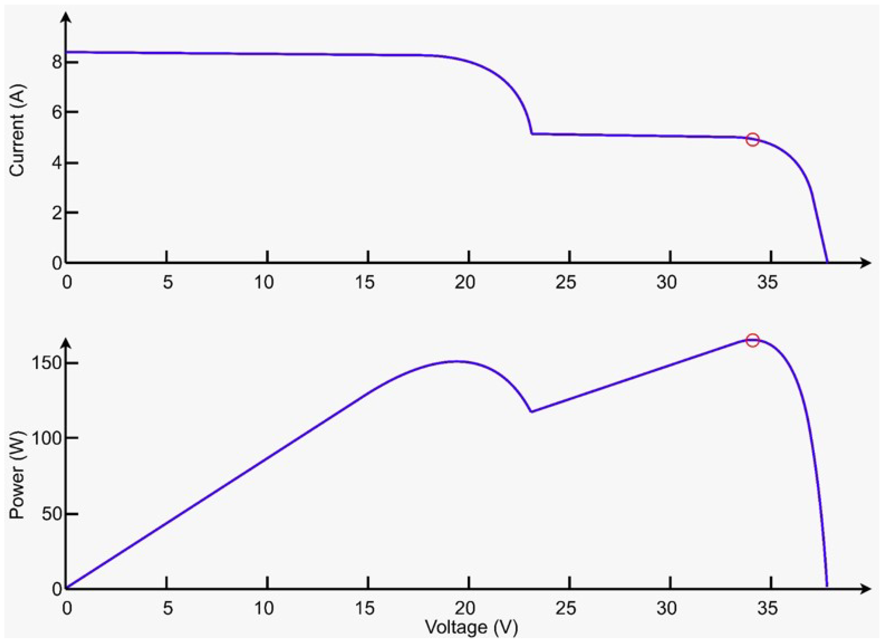
Figure 5.
Experimental facility. (a) Front view. (b) Rear view. Reprinted from Ruiz et al. [20] with permission from Elsevier, 2020.
Figure 5.
Experimental facility. (a) Front view. (b) Rear view. Reprinted from Ruiz et al. [20] with permission from Elsevier, 2020.
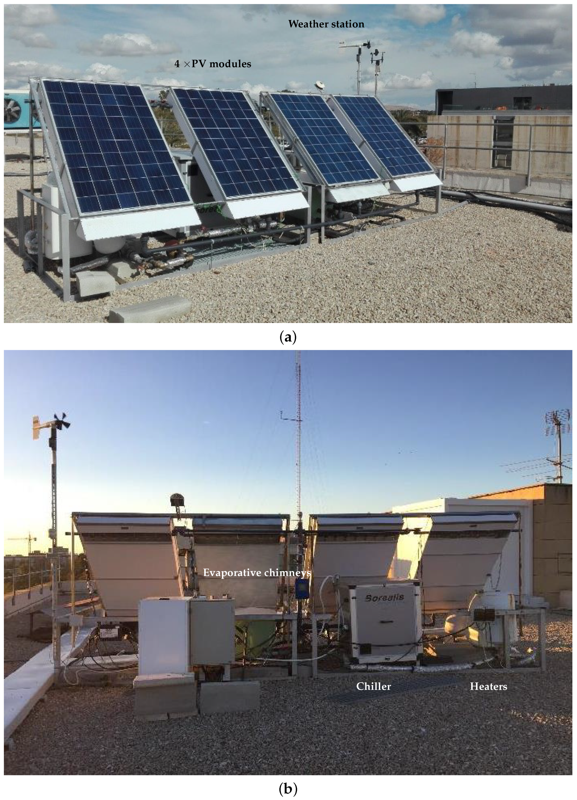
Figure 6.
Schematic diagram of the experimental measuring equipment. Reprinted from Ruiz et al. [20] with permission from Elsevier, 2020.
Figure 6.
Schematic diagram of the experimental measuring equipment. Reprinted from Ruiz et al. [20] with permission from Elsevier, 2020.
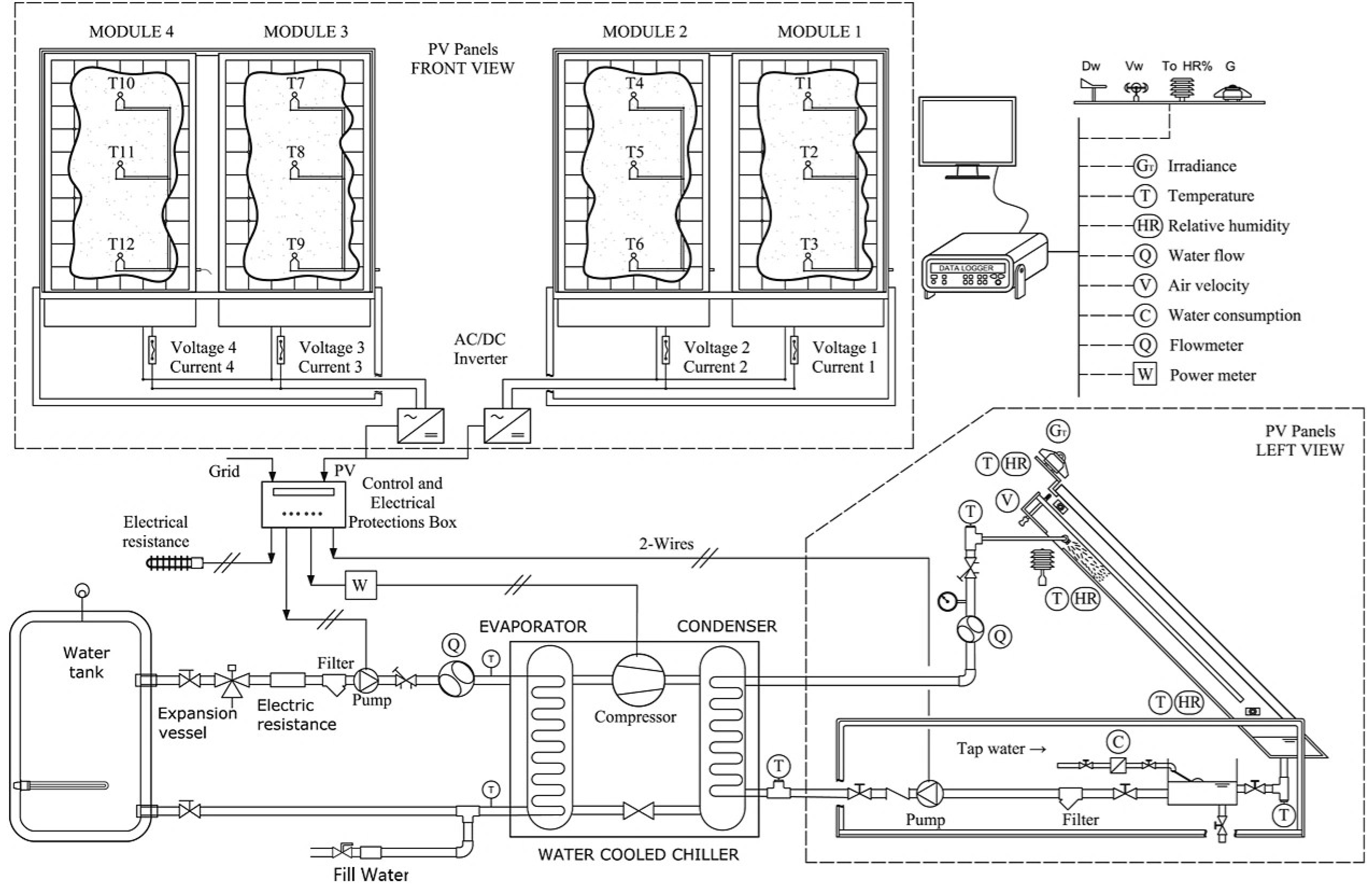
Figure 7.
I–V curve tracer block diagram.

Figure 8.
I–V curve tracer system (not assembled).

Figure 9.
Thermographic evaluation of the module temperature distribution. (a) Evaporative chimney on and (b) evaporative chimney off.
Figure 9.
Thermographic evaluation of the module temperature distribution. (a) Evaporative chimney on and (b) evaporative chimney off.

Figure 10.
Temporal evolution of the (a) I–V and (b) P–V curves measured with chimney activated during 1 experimental test.
Figure 10.
Temporal evolution of the (a) I–V and (b) P–V curves measured with chimney activated during 1 experimental test.
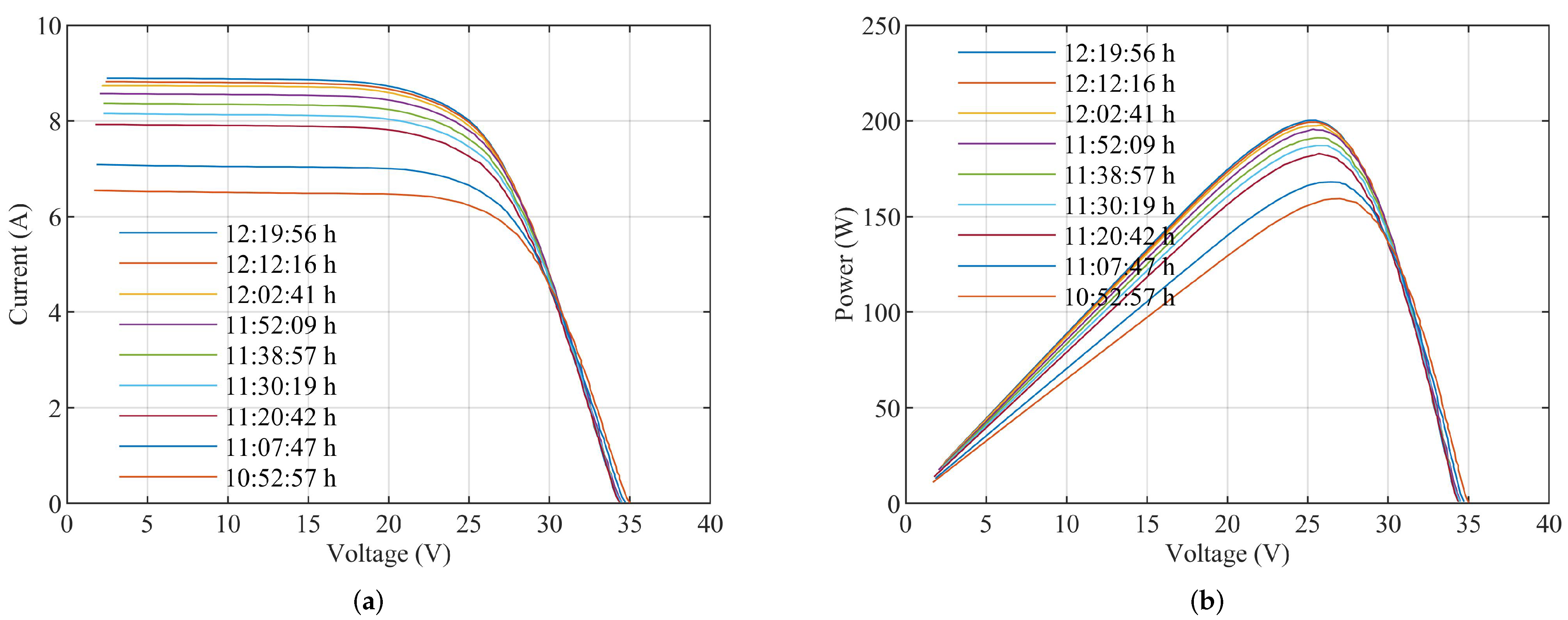
Figure 11.
(a) I–V curves comparison with chimney activated and deactivated. (b) P–V curves comparison with chimney activated and deactivated.
Figure 11.
(a) I–V curves comparison with chimney activated and deactivated. (b) P–V curves comparison with chimney activated and deactivated.

Figure 12.
Maximum power available for different irradiance levels with the chimney activated and deactivated.
Figure 12.
Maximum power available for different irradiance levels with the chimney activated and deactivated.

Table 1.
Sunrise SR-660255 specifications.
| Magnitude | Units | Value |
|---|---|---|
| Maximum power | W | 255 |
| Dimensions | mm | 1637 × 992 × 40 |
| Number of cells | - | 60 |
| Number of diodes | - | 6 |
| Cell type | - | Polycrystalline |
| Module efficiency | % | 15.7 |
| Short-circuit current | A | 9.11 |
| Open-circuit voltage | V | 37.49 |
| Nominal voltage | V | 30.24 |
| Nominal current | A | 8.44 |
Table 2.
Measuring equipment used in the experimental tests.
| Variable | Brand-Model | Sensor Type | Range | Accuracy |
|---|---|---|---|---|
| Ambient air temperature | E+E Elektronik (EE 21) | Capacitive sensor | −20–80 °C | ±0.3 °C |
| Ambient air relative humidity | E+E Elektronik (EE 21) | Capacitive sensor | 0–100% | % |
| Wind direction | Young (05103L) | Balanced vane | 0–360° | |
| Wind speed | Young (05103L) | 4-blade helicoid propeller | 0–50 m/s | m/s |
| Irradiance | Kipp&Zonen CM-6B | First-class pyranometer | 0–1400 W/m | % RD |
Publisher’s Note: MDPI stays neutral with regard to jurisdictional claims in published maps and institutional affiliations. |
© 2021 by the authors. Licensee MDPI, Basel, Switzerland. This article is an open access article distributed under the terms and conditions of the Creative Commons Attribution (CC BY) license (https://creativecommons.org/licenses/by/4.0/).
Share and Cite
MDPI and ACS Style
Casado, P.; Blanes, J.M.; Valero, F.J.A.; Torres, C.; Lucas Miralles, M.; Ruiz Ramírez, J. Photovoltaic Evaporative Chimney I–V Measurement System. Energies 2021, 14, 8198. https://doi.org/10.3390/en14248198
AMA Style
Casado P, Blanes JM, Valero FJA, Torres C, Lucas Miralles M, Ruiz Ramírez J. Photovoltaic Evaporative Chimney I–V Measurement System. Energies. 2021; 14(24):8198. https://doi.org/10.3390/en14248198
Chicago/Turabian StyleCasado, Pablo, José M. Blanes, Francisco Javier Aguilar Valero, Cristian Torres, Manuel Lucas Miralles, and Javier Ruiz Ramírez. 2021. "Photovoltaic Evaporative Chimney I–V Measurement System" Energies 14, no. 24: 8198. https://doi.org/10.3390/en14248198
Note that from the first issue of 2016, this journal uses article numbers instead of page numbers. See further details here.