Optimization Algorithm of Effective Stress Coefficient for Permeability

Abstract

The effective stress coefficient for permeability is a significant index for characterizing the variation in permeability with effective stress. The realization of its accuracy is essential for studying the stress sensitivity of oil and gas reservoirs. The determination of the effective stress coefficient for permeability can be mainly evaluated using the cross-plotting or response surface method. Both methods preprocess experimental data and preset a specific function relation, resulting in deviation in the calculation results. To improve the calculation accuracy of the effective stress coefficient for permeability, a 3D surface fitting calculation method was proposed according to the linear effective stress law and continuity hypothesis. The statistical parameters of the aforementioned three methods were compared, and the results showed that the three-dimensional (3D) surface fitting method had the advantages of a high correlation coefficient, low root mean square error, and low residual error. The principal of using the 3D surface fitting method to calculate the effective stress coefficient of permeability was to evaluate the influence of two independent variables on a dependent variable by means of a 3D nonlinear regression. Therefore, the method could be applied to studying the relationship between other physical properties and effective stress.

1. Introduction

Effective stress has always been a notable research topic in pore elastomechanics theory, which has substantial guiding significance for oil and gas development and is widely used in reservoir numerical simulations, oil and gas productivity prediction, and reservoir reconstruction.

Terzaghi [1] first proposed the expression of effective stress as follows:

$${\sigma }_{eff}^T=\sigma -P,$$

(1)

Equation (1) is suitable for studying the settlement of loose soil and mechanical failure of most rocks. However, the cementation mode, pore structure, and compressibility of rock in oil and gas reservoirs differ from those of soil, and thus Equation (1) is not suitable to express effective stress.

According to the theory of Biot [2,3] and the principle of stress–strain superposition, Nur [4] derived an accurate expression of the effective stress applicable to the elastic deformation of pores:

$${\sigma }_{eff}=\sigma -\alpha P,$$

(2)

where α is the Biot coefficient, σ_eff is the effective stress (MPa), σ is the overlying stress or confining pressure (MPa), and P is the pore fluid pressure (MPa).

Many theoretical and experimental studies have shown that the predicted value of the Biot coefficient is less than 1 [3,5,6]. For rocks in general, the Biot coefficient is between 0.12 and 0.91. The Biot coefficient of effective stress mainly focuses on measuring the pore elastic parameters of rock and represents the degree of the relative influence of pore fluid pressure and overburdened pressure on the pore elastic parameters.

However, the effective stress coefficient is less than 1, which is not applicable to all types of rock. Ghabezloo [7], Meng [8], Wang [9], Li Min and Xiao Wenlian et al. [10] found that the effective stress coefficient was greater than 1 when they tested the permeability of rocks containing clay minerals, which indicated that the influence of pore fluid pressure on permeability was greater than confining pressure.

According to various scholars including Berryman [11], Robin [12], and Bernabe [13,14], there is no uniform law of effective stress for different physical properties, and the effective stress coefficients differ significantly. Therefore, different symbols should be used to represent the effective stress coefficients for different physical properties. When using permeability as the research object, such coefficient should be called the effective stress coefficient for permeability (ESCP, expressed as α_k to distinguish it from the Biot coefficient).

Bernabe [13,14] first proposed the concept of effective stress for permeability and then expressed the relationship among permeability and effective stress, confining pressure, and pore pressure as follows:

$$k=f_k\left(\sigma ,P\right)=f_k\left({\sigma }_{eff}\right)=f_k\left(\sigma -{\alpha }_{k}P\right),$$

(3)

where α_k is ESCP, which reflects the relative magnitude of the influence of pore fluid pressure and confining pressure on permeability.

The calculation of the ESCP is helpful for studying the deformation law and seepage characteristics of reservoir rock. This calculation is the basis of the evaluation of reservoir stress sensitivity and is of great significance for oil and gas productivity evaluation and efficient development [15,16].

2. Calculation Methods for the ESCP

The determination of the ESCP depends on the test data obtained from the stress-sensitive experiment. The ESCP can be obtained after the data are processed using the cross-plotting method [17] or the response surface method [18].

2.1. Cross-Plotting Method

Walsh [17] used the cross-plotting method to calculate the effective stress coefficient while studying the permeability of fractured rock that changed with the confining and pore fluid pressures. The main steps of this method are as follows.

(1) Linear fitting was performed for determining the relationship between $k^{-\frac{1}{3}}$ and pore fluid pressure under different confining pressures.

(2) In the linear diagram of the relationship between $k^{-\frac{1}{3}}$ and pore fluid pressure, isolines of several groups of permeability were drawn, and the confining pressure and pore fluid pressure under the same permeability could be obtained by cross-plotting.

(3) The relationship between the confining pressure and pore fluid pressure under the same permeability was linearly fitted, and the slope of the linear relationship between the confining pressure and pore fluid pressure was determined as the effective stress coefficient. The effective stress coefficient of the rock sample was obtained by averaging several groups of the ESCP.

The cross-plotting method implies two prerequisites: first, the effective stress should be linear, that is, Equation (2), and second, the relationship of permeability with effective stress was preset as follows [17]:

$${\left(\frac{k}{k_0}\right)}^{\frac{1}{3}}=1-\frac{\sqrt{2}h}{a_0}ln\left(\frac{{\sigma }_{eff}}{{\sigma }_{{eff}_0}}\right),$$

(4)

where $k_0$ and $a_0$ are the permeability and half-width of the crack at a reference stress ${\sigma }_{{eff}_0}$, respectively, and h is the root mean square of the height distribution of the crack surface. Jones [19] demonstrated Equation (4) in an experimental study of fractured carbonate rocks. Equation (4) was derived by Walsh [17,20] and is based on the plate fracture model, considering fracture roughness. Therefore, Equation (4) is mainly applicable to fractured rocks.

2.2. Response Surface Method

Xiao [18] and Li [21,22] used the response surface method to investigate the stress sensitivity and effective stress coefficient of tight sandstone. The steps of this method are as follows.

(1) Transform the permeability or volumetric strain data into a simpler form and appropriately weight the variance.

$$k^{\prime }=k^{\lambda },$$

(5)

where k is the original experimental data of permeability, k′ is the converted permeability data, and λ demonstrates power, which is typically between −3 and +3. A transformation can simplify the surface or standardize the known variances or errors in the data; however, this must be performed carefully to avoid skewing the statistical analysis.

(2) Fit the converted data to the quadric surface for both σ and P:

$$k^{\prime }=x_1+x_2\sigma +x_{3}P+x_4{\sigma }^2+x_5\sigma P+x_6{P}^2,$$

(6)

where x_i coefficients are determined from the fit.

(3) Statistical parameters and quadric surface figures were used to infer the physical and mechanical effects, permeability evolution, and effective stress coefficients of rock.

Equation (6) could be simplified as follows:

$$k^{\prime }=y_1{\left(\sigma -y_{2}P\right)}^2+y_3\left(\sigma -y_{2}P\right)+y_4,$$

(7)

where y_i coefficients are determined from the fit. Equation (6) can be derived by expanding Equation (7).

By introducing an intermediate variable (i.e., effective stress σ_k), Equations (6) and (7) can be written as follows:

$${\sigma }_k=\sigma -y_{2}P,$$

(8)

$$k^{\prime }=y_1{\left({\sigma }_k\right)}^2+y_3\left({\sigma }_k\right)+y_4,$$

(9)

Equations (8) and (9) demonstrate that the response surface method implies two conditions for use: first, the effective stress should be linear, that is, Equation (2), and second, the evolution of permeability with effective stress is assumed to be a quadratic polynomial function. Therefore, the essence of the response surface method is to use a bivariate quadratic polynomial to fit the experimental data and then obtain statistical parameters and effective stress coefficients.

The aforementioned analysis showed that the calculation of the effective stress coefficient by the cross-plotting method and response surface method had the following defects:

(1) The specific functional relationship between permeability and effective stress could not satisfy the experimental data for all rock types.

(2) Preprocessing of the original experimental data may lead to fitting errors and even distortion of the analysis results.

2.3. 3D Surface Fitting Method

On the basis of defects of the cross-plotting method and response surface method, this study proposes a method of fitting experimental data with a 3D surface to obtain the effective stress coefficient.

The functional relationship between rock permeability and effective stress could be expressed as follows:

$$k=f_k\left(\sigma -{\alpha }_{k}P\right),$$

(10)

Equation (10) mainly contains three types:

(1) Power law model [23,24]

$$k=b{\left(\sigma -aP\right)}^{-c},$$

(11)

(2) Exponential model [25]

$$k=c{e}^{-b\left(\sigma -aP\right)},$$

(12)

(3) Quadratic polynomial model [26]

$$k=b{\left(\sigma -aP\right)}^2+c\left(\sigma -aP\right)+d,$$

(13)

where $a$, b, c, and d are fitting parameters, and $a$ is the ESCP of each model.

An assumption was that the effective stress linearly correlated with the confining and pore fluid pressures, satisfying Equation (2). Assuming that Equation (10) is continuously differentiable within the range of the stress variation,

$$dk=\frac{\partial k}{\partial \sigma }d\sigma +\frac{\partial k}{\partial p}dP=\frac{dk}{d{\sigma }_{eff}}·d\sigma -{\alpha }_k·\frac{dk}{d{\sigma }_{eff}}·dP,$$

(14)

The ESCP represents the relative influence of pore fluid and confining pressures on permeability, which was used to evaluate the contribution of two independent variables (σ, P) to a dependent variable (k). The ESCP can be expressed as the ratio of the partial derivative coefficients of the two independent variables:

$$\left(\frac{\partial k}{\partial P}\right)/\left(\frac{\partial k}{\partial \sigma }\right)=\left(-{\alpha }_k\frac{dk}{d{\sigma }_{eff}}\right)/\left(\frac{dk}{d{\sigma }_{eff}}\right)=-{\alpha }_k,$$

(15)

$${\alpha }_k=-\left(\frac{\partial k}{\partial P}\right)/\left(\frac{\partial k}{\partial \sigma }\right),$$

(16)

The calculation of the ESCP was transformed into the problem of fitting the 3D surface of experimental data on the confining pressure, pore fluid pressure, and permeability. The Curve Fitting toolbox in MATLAB was used to fit the experimental data through three models, and three fitting parameters, a, were obtained. Finally, the a in the optimal fitting scheme was selected as the ESCP of the rock sample.

The 3D surface fitting method is proposed according to linear effective stress law and continuity hypothesis. If the effective stress cannot be expressed by the linear relationship between confining pressure and pore pressure, the 3D surface fitting method is no longer applicable.

3. Results

The experimental data of two tight sandstones (rock samples 1 and 2, from Qiao [27]) and two lithic sandstones (rock samples D13−4 and D15−2, from Xiao [18]) were selected.

Two tight sandstones from British Columbia, Canada, were Jurassic sandstones. The samples were dark gray and mainly consisted of quartz, black silica, and feldspar clasts. The porosity of the sandstone ranged from 1.65% to 3.23%. The rock samples were cylindrical specimens with a diameter of 38 mm and a height of 51 mm. The experimental data for rock samples 1 and 2 are listed in

Table 1. Stress sensitivity experimental data of rock samples 1 and 2.

σ/MPa	P/MPa	k/mD
		Sample 1	Sample 2
10	2	0.00533	0.00631
10	5	0.0113	0.0142
10	8	0.019	0.0182
20	4	0.0042	0.00324
20	8	0.00932	0.0073
20	12	0.0151	0.0155
20	16	0.0309	0.03
30	5	0.00487	0.0024
30	10	0.00551	0.00421
30	15	0.0103	0.0115
30	20	0.015	0.014
30	25	0.0307	0.0313
ESCP was obtained by the cross-plotting method		0.509	0.612

.

The 3D surface fitting method was used to fit the experimental data of the two rock samples (Table 1).

Table A1. Accuracy and calculation results of 3D surface fitting method (rock samples 1 and 2).

Rock Sample	Model	R2	RMSE	Calculation Results of 3D Surface Fitting Method	Calculation Results of Cross-Plotting Method
Sample 1	quadratic polynomial	0.9206	0.003083	1.551	0.509
Sample 1	exponential	0.9085	0.003121	1.507	0.509
Sample 1	power law	-	-	-	0.509
Sample 2	quadratic polynomial	0.9333	0.002921	1.539	0.612
Sample 2	exponential	0.9085	0.003121	1.507	0.612
Sample 2	power law	-	-	-	0.612

in the Appendix A lists the precision and calculation results of different fitting functions, and Figure 1 shows the corresponding fitting curves.

Two lithic sandstones were taken from the Permian and buried at a depth of approximately 2700 m. The porosity of D13−4 was 6.48%, and that of D15−2 was 6.88%. Experimental data and calculation results of the lithic sandstones are shown in

Table A2. Stress sensitivity test data (rock sample D13−4 from Xiao [18]).

σ/MPa	P/MPa	k/mD	σ/MPa	P/MPa	k/mD
51.00	26.02	0.21032	45.00	10.35	0.19216
51.00	22.46	0.18967	45.00	14.35	0.19428
51.00	18.15	0.17284	45.00	18.44	0.20139
51.00	14.01	0.15984	45.00	22.41	0.20740
51.00	10.24	0.14886	45.00	26.50	0.23058
51.00	6.01	0.14468	39.00	26.58	0.42405
51.00	10.09	0.14444	39.00	22.49	0.37336
51.00	14.23	0.14734	39.00	18.47	0.33524
51.00	18.24	0.15184	39.00	14.50	0.30324
51.00	22.31	0.16027	39.00	10.34	0.27396
51.00	26.08	0.17022	39.00	6.32	0.25667
45.00	26.51	0.30610	39.00	10.31	0.26015
45.00	22.41	0.27366	39.00	14.45	0.27361
45.00	18.31	0.23324	39.00	18.42	0.28018
45.00	14.18	0.21248	39.00	22.53	0.30107
45.00	10.22	0.19993	39.00	26.54	0.32863
45.00	6.24	0.19301

ESCP is obtained by response surface method: 0.25920.

and

Table A3. Stress sensitivity test data (rock sample D15−2 from Xiao [18]).

σ/MPa	P/MPa	k/mD	σ/MPa	P/MPa	k/mD
12.00	10.19	0.06359	42.00	19.81	0.01131
17.00	10.19	0.03808	47.00	19.79	0.00962
22.00	10.12	0.02416	52.00	19.73	0.00871
27.00	10.05	0.01733	47.00	19.77	0.00915
32.00	9.98	0.01350	42.00	19.82	0.01035
37.00	9.92	0.01140	37.00	19.89	0.01254
42.00	9.87	0.00998	32.00	19.96	0.01671
47.00	9.85	0.00896	27.00	20.12	0.02621
52.00	9.82	0.00819	22.00	20.13	0.04885
47.00	9.34	0.00846	27.00	25.13	0.04658
42.00	9.85	0.00904	32.00	25.20	0.02961
37.00	9.93	0.00980	37.00	25.00	0.01979
32.00	9.96	0.01094	42.00	24.92	0.01412
27.00	10.00	0.01318	47.00	24.83	0.01130
22.00	10.07	0.01813	52.00	24.75	0.00964
17.00	10.15	0.02907	47.00	24.79	0.01036
12.00	10.19	0.05745	42.00	24.91	0.01247
17.00	15.18	0.06110	37.00	25.01	0.01640
22.00	15.11	0.03592	32.00	25.06	0.02511
27.00	15.07	0.02268	27.00	25.19	0.04535
32.00	14.98	0.01650	32.00	30.08	0.04340
37.00	14.90	0.01315	37.00	30.05	0.02762
42.00	14.87	0.01095	42.00	29.93	0.01842
47.00	14.76	0.00934	47.00	29.85	0.01311
52.00	14.73	0.00857	52.00	29.75	0.01039
47.00	14.73	0.00898	47.00	29.81	0.01196
42.00	14.77	0.00966	42.00	29.91	0.01542
37.00	14.84	0.01169	37.00	30.00	0.02328
32.00	14.88	0.01365	32.00	30.08	0.04093
27.00	14.97	0.01880	37.00	35.04	0.04064
22.00	15.09	0.03031	42.00	34.96	0.02616
17.00	15.13	0.05882	47.00	34.84	0.01635
22.00	20.25	0.05688	52.00	34.71	0.01247
27.00	20.11	0.03019	47.00	34.79	0.01508
32.00	20.03	0.01948	42.00	35.00	0.02260
37.00	19.92	0.01455	37.00	35.11	0.03903

ESCP is obtained by response surface method: 0.6497.

in the Appendix A.

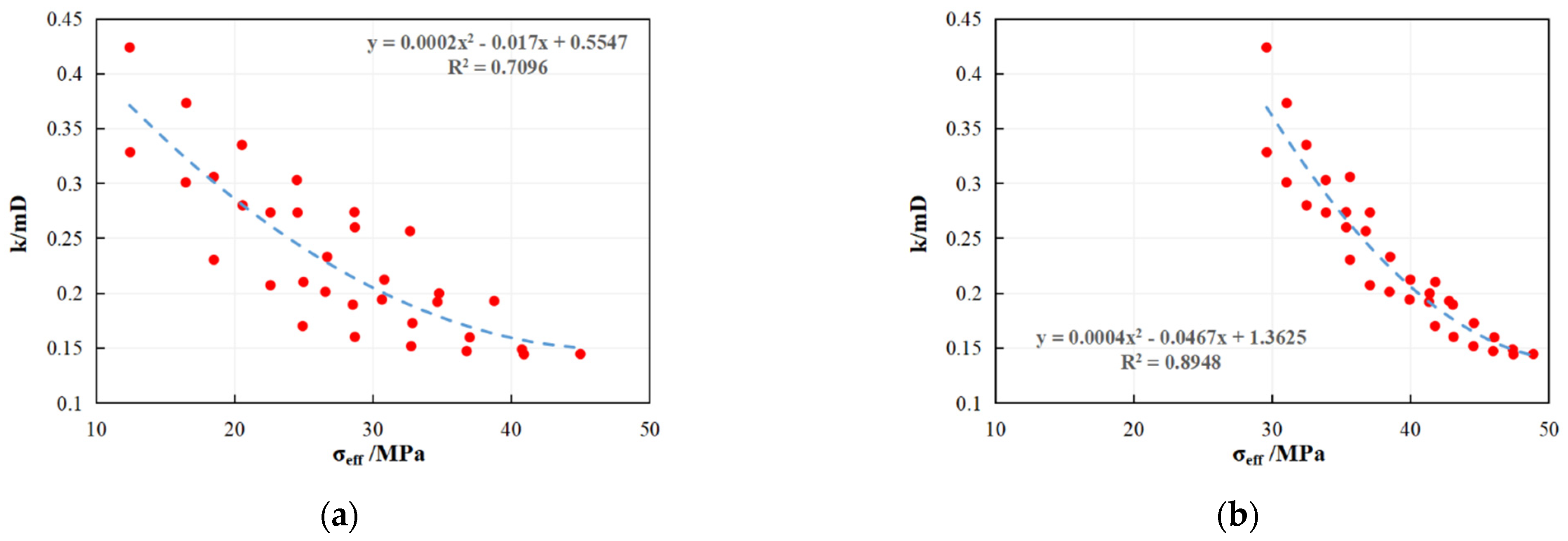
The 3D surface fitting method was used to fit the experimental data of the two rock samples, D13−4 and D15−2.

Table A4. Accuracy and calculation results of 3D surface fitting method (rock sample D13−4 and D15−2).

Rock Sample	Model	R2	RMSE	Calculation Results of 3D Surface Fitting Method	Calculation Results of Response Surface Method
D13−4	power law	0.8952	0.02397	0.3388	0.25920
D13−4	quadratic polynomial	0.8948	0.02442	0.3537	0.25920
D13−4	exponential	0.8924	0.02428	0.3518	0.25920
D15−2	power law	0.9741	0.002434	0.9002	0.6497
D15−2	quadratic polynomial	0.9428	0.003613	0.7978	0.6497
D15−2	exponential	0.9367	0.003828	0.7767	0.6497

in the Appendix A lists the precision and calculation results of the different fitting functions. The ESCP of rock samples D13−4 and D15−2 was set as 1, three functional relationships were used to fit the experimental data; the fitting correlation coefficients were all lower than that of the 3D surface fitting method. Figure 2 and Figure 3 list part of fitting curves of the two rock samples.

Figure 2 shows that the fitting correlation coefficient is only 0.7096 when the ESCP is set as 1. It cannot accurately describe the variation law of sandstone permeability with confining and pore fluid pressures if the effective stress coefficient is set as 1. Therefore, the first step in the evaluation of stress sensitivity of reservoir permeability involves obtaining the ESCP based on the experimental data, and the second step involves the evaluation of reservoir stress sensitivity.

Figure 3a,b shows that when the permeability is between 0.03 and 0.05 mD, the 3D surface fitting method has a better effect than the response surface method. When the effective stress coefficient was set to 0.6479, most data points were not on the fitting surface.

Figure 1, Figure 2 and Figure 3 demonstrate that the fitting effect of the 3D surface fitting method is better than the cross-plotting method and response surface method. The following section presents a quantitative analysis of the various methods from the perspective of data statistics.

4. Discussion

The accuracy and reliability of the 3D surface fitting method, cross-plotting method, and response surface method were quantitatively analyzed by selecting three common statistical parameters: correlation coefficient, root mean square error (RMSE), and residual error.

4.1. Comparison of the 3D Surface Fitting Method and Cross-Plotting Method

The ESCP values of rock samples 1 and 2 obtained by the 3D surface fitting method are 1.551 and 1.539, respectively. The results obtained by the different fitting types are relatively stable and consistent (Table A1 in the Appendix A). The ESCPs of rock samples 1 and 2 obtained by the cross-plotting method were 0.509 and 0.612, respectively. An ESCP of less than 1 indicates that the pore fluid pressure has less effect on permeability than the confining pressure; more than 1 means the opposite. The results obtained by the two methods are the opposite. The original experimental data must be analyzed to determine which method is the most reliable.

Three groups of experimental data were selected (

Table 2. Comparison of the effects of confining and pore fluid pressures on permeability (samples 1 and 2).

σ/MPa	P/MPa	k/mD		∆σ/MPa		∆k/mD
		Sample 1	Sample 2	Sample 1	Sample 2	Sample 1	Sample 2
10	5	0.0113	0.0142	20	20	0.00643	0.0118
30	5	0.00487	0.0024	-	-	-	-
30	25	0.0307	0.0313	20	20	0.02583	0.0289

). Using the permeability under a confining pressure of 30 MPa and pore fluid pressure of 5 MPa as a reference, the permeability change values were obtained when the confining pressure was reduced by 20 MPa, and the pore fluid pressure was increased by 20 MPa, respectively. The changing values of the confining and pore fluid pressures were the same. If the change in permeability during the period of change in the pore fluid pressure is greater than that during confining pressure change, the pore fluid pressure has a greater influence on permeability, and the ESCP should be greater than 1.

The calculation results in Table 2 show that when the pore fluid pressure changes by 20 MPa, the permeability change values of rock samples 1 and 2 are 0.02583 and 0.0289 mD, respectively. When the confining pressure changes by 20 MPa, the permeability change values of rock samples 1 and 2 are 0.00643 and 0.0118 mD, respectively. The effect of pore fluid pressure on permeability is significantly greater than that of confining pressure; that is, the ESCPs of rock samples 1 and 2 are greater than 1.

The ESCP calculated using the cross-plotting method is inconsistent with the experimental data. The main reason for this deviation is that if the original data points cannot coincide with the cross plot, the confining and pore fluid pressures of the cross point must be calculated using the interpolation method. Bernabe [13] pointed out that the stress–permeability data were too scattered and that interpolation could lead to statistical errors; thus, interpolation was generally applied to stress–strain analysis.

4.1.1. Comparison of Three Fitting Functions

Three functions were used to fit the experimental data of rock samples 1 and 2. The quadratic polynomial type had the highest correlation coefficient, followed by the exponential type, and the power law type had a negative correlation coefficient. The relationship between permeability and effective stress in rock samples 1 and 2 did not agree with the power law function.

The quadratic polynomial model that Yin and Wang [26] proposed was based on the thick-walled tube theory, mainly used to describe the quadratic parabolic relationship between permeability and effective stress of capillary rock. The matrix rock and fractured rock can be described by exponential and power law models, respectively. Zhao [28] and Dong have posited that the logarithmic, quadratic polynomial, and power law models are the best for characterizing fractured rock, porous tight sandstone, and fine-grained sandstone, respectively.

The power law model, introduced by Shi [24], was using to fit experimental data and achieved good results. However, Xiao [18] and Dong [23] have pointed out that the power law relationship is an empirical formula based on the fitting of experimental data, without clear physical meaning and theoretical support. The fitting results in this study also showed that the power law relation was invalid and not universally applicable.

David et al. [25] discussed the exponential model in detail and posited that the exponential relation is an empirical formula based on experimental data. When the experimental pressure was less than the critical pressure, the equation was in good agreement with the experimental data. Notably, the exponential model can be simplified using Equation (18).

McKee et al. [29] deduced the following formulas for the functional relationships between the effective stress and two factors, porosity and permeability:

$$\varphi ={\varphi }_0\frac{e^{-{\overline{c}}_p∆\sigma }}{1-{\varphi }_0\left(1-e^{-{\overline{c}}_p∆\sigma }\right)},$$

(17)

$$k=k_0\frac{e^{-3{\overline{c}}_p∆\sigma }}{1-{\varphi }_0\left(1-e^{-{\overline{c}}_p∆\sigma }\right)},$$

(18)

where ${\varphi }_0$ and $k_0$ are the porosity and permeability when the effective stress is 0, ${\overline{c}}_p$ is the average pore compressibility, and ∆σ is the change in the effective stress. Because the initial porosity of tight sandstone is small, Equation (18) can be simplified as follows:

$$\varphi ={\varphi }_0\frac{e^{-{\overline{c}}_p∆\sigma }}{1-{\varphi }_0\left(1-e^{-{\overline{c}}_p∆\sigma }\right)},$$

(19)

Equation (19) is an exponential model that is simple in mathematical form, easy to use, and widely used to fit stress-sensitive experimental data.

Table A5. Research status of experiment for pressure sensitivity.

Reference	Year	Rock Type	Fitting Model
			Exponential	Power Law	Quadratic Polynomial
Reyes [31]	2002	shale	exponential
Chalmers [32]	2012	shale	exponential
Dong [23]	2013	shale		power law
Xiao [18]	2013	sandstone	exponential	power law	quadratic polynomial
Dou [33]	2016	-	exponential
Lu et al. [34]	2020	sandstone		power law
Zheng et al. [35]	2020	shale	exponential

in the Appendix A lists the experimental research information on stress sensitivity. Many experimental results have demonstrated that this simplification was acceptable for rocks with small initial porosity.

4.1.2. Correlation Coefficient and RMSE

The ESCP obtained by the cross-plotting and 3D surface fitting methods was used to fit the experimental data. The correlation coefficient (R²) and RMSE are listed in

Table 3. Correlation coefficient and RMSE of different methods (rock samples, 1 and 2).

Method	Sample	Model	ESCP	R2	RMSE
3D surface fitting	1	Quadratic polynomial	1.551	0.9206	0.003083
	1	Exponential	1.551	0.9085	0.003121
	2	Quadratic polynomial	1.539	0.9333	0.002921
	2	Exponential	1.539	0.9085	0.003121
Cross-plotting	1	Quadratic polynomial	0.509	0.2066	0.009189
	1	Exponential	0.509	0.0928	0.009321
	2	Quadratic polynomial	0.612	0.2955	0.008951
	2	Exponential	0.612	0.1494	0.009026

.

In Table 3, the correlation coefficients of the 3D surface fitting method are all greater than 0.9, and the correlation coefficients of the cross-plotting method are less than 0.3. The larger the correlation coefficients, the closer the statistical results are to the actual situation. The RMSE of the 3D surface fitting method is approximately 0.003, and that of the cross-plotting method is approximately 0.009, which is three times that of the former. The bigger the RMSE, the bigger the difference between the statistical results and the actual situation is. Comparing the correlation coefficient and RMSE of the two methods demonstrates the advantages of the 3D surface fitting method.

4.1.3. Residual Error

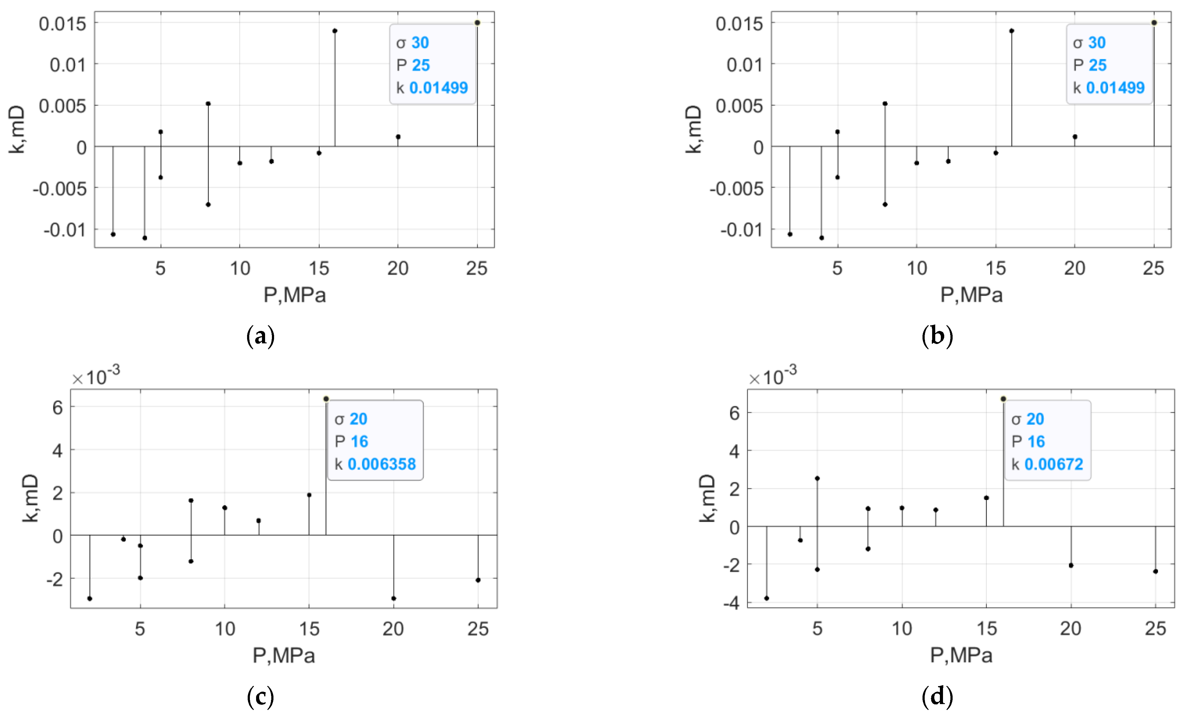
To directly reflect the difference between the cross-plotting and 3D surface fitting methods, distribution maps of the residual error for the two methods under different fitting relations were drawn (Figure 4 and Figure 5).

Figure 4a,b shows that the residual error of the cross-plotting method ranges from −0.012 to 0.018, and the maximum residual error is 0.01784. Figure 4c,d shows that the distribution interval of the residual error of the 3D surface fitting method is from −0.004 to 0.0068, and the maximum value is 0.00672. The scope and maximum value of the residual error of the 3D surface fitting method are smaller than those of the cross-plotting method by nearly three times.

Figure 5a,b shows that the residual error of the cross-plotting method ranges from −0.012 to 0.018, and the maximum residual error is 0.01736. Figure 5c,d shows that the distribution interval of the residual error of the 3D surface fitting method is from −0.004 to 0.0068, and the maximum value is 0.00672. The scope and maximum value of the residual error of the 3D surface fitting method are nearly three times smaller than those of the cross-plotting method, indicating that the accuracy and reliability of the 3D surface fitting method are much higher than those of the cross-plotting method.

Comparative analysis of the three statistical parameters shows that the ESCP obtained by the cross-plotting method cannot accurately fit the experimental data of rock, and the correlation coefficients are less than 0.3. The correlation coefficients of the 3D surface fitting method were all greater than 0.9, demonstrating the method’s benefit.

4.2. Comparison of the 3D Surface Fitting Method and Response Surface Method

Table A4 in the Appendix A lists the precision and calculation results of the 3D surface fitting method using different fitting functions. The fitting accuracy of the power law type is the highest, but the calculation results of the effective stress coefficient significantly differ from those of the other two types. The exponential and quadratic polynomial models have the theoretical basis support, the difference in calculation result is small. The power law relation had no theoretical basis and failed to fit rock samples 1 and 2. Therefore, the exponential and quadratic polynomial models are more reliable than the power law relation. In this study, the power law relation was not considered in the calculation of ESCP.

The ESCP values of rock samples D13−4 and D15−2 obtained by the 3D surface fitting method were 0.3537 and 0.7767, respectively. The ESCP values of rock samples D13−4 and D15−2 obtained by the response surface method were 0.2592 and 0.6497 [18], respectively.

4.2.1. Correlation Coefficient and RMSE

The ESCPs obtained by the response surface and 3D surface fitting method were used to fit the test data of samples D13−4 and D15−2. The correlation coefficient and RMSE are listed in

Table 4. Correlation coefficient and RMSE of different methods (rock samples D13−4 and D15−2).

Method	Sample	Model	ESCP	R2	RMSE
3D surface fitting	D13−4	Quadratic polynomial	0.3537	0.8948	0.02442
	D13−4	Exponential	0.3518	0.8924	0.02428
	D15−2	Quadratic polynomial	0.7767	0.9367	0.003828
	D15−2	Exponential	0.7978	0.9428	0.003613
response surface	D13−4	Quadratic polynomial	0.2592	0.8845	0.02515
	D13−4	Exponential	0.2592	0.8824	0.02497
	D15−2	Quadratic polynomial	0.6497	0.9193	0.004293
	D15−2	Exponential	0.6497	0.9185	0.004282

.

For rock sample D13−4, whether a quadratic polynomial model or exponential model is used for fitting, the correlation coefficient of the 3D surface fitting method is larger than that of the response surface method, while the RMSE is smaller than that of the response surface method. The same situation is observed in rock sample D15−2.

The comparison of the correlation coefficient and RMSE of the two methods showed a slightly improved data processing accuracy when using the 3D surface fitting method.

4.2.2. Residual Error

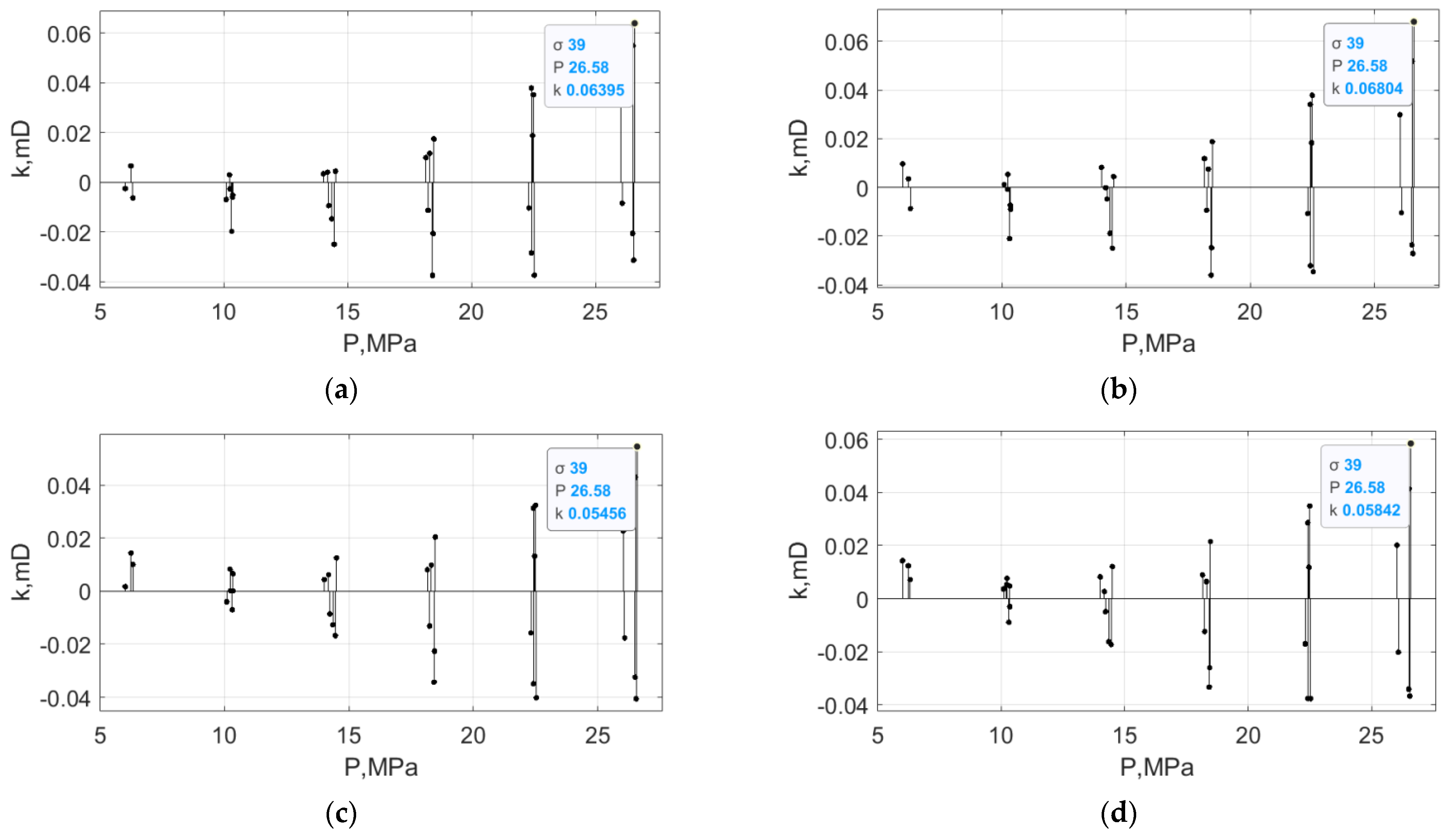
Experimental data of rock samples D13−4 and D15−2 were processed to draw residual error distribution maps of the response surface and 3D surface fitting methods by using different fitting functions (Figure 6 and Figure 7).

In Figure 6a,b, the distribution range of the residual error of the response surface method is from −0.04 to 0.07, and the maximum value of the residual error is 0.06804. Figure 6c,d shows that the distribution interval of the residual error of the 3D surface fitting method is from −0.04 to 0.06, and the maximum value of the residual error is 0.05842. The distribution interval and maximum value of the residual error of the latter are approximately 0.01 smaller than those of the former, indicating that the fitting accuracy of the latter is slightly higher than that of the former.

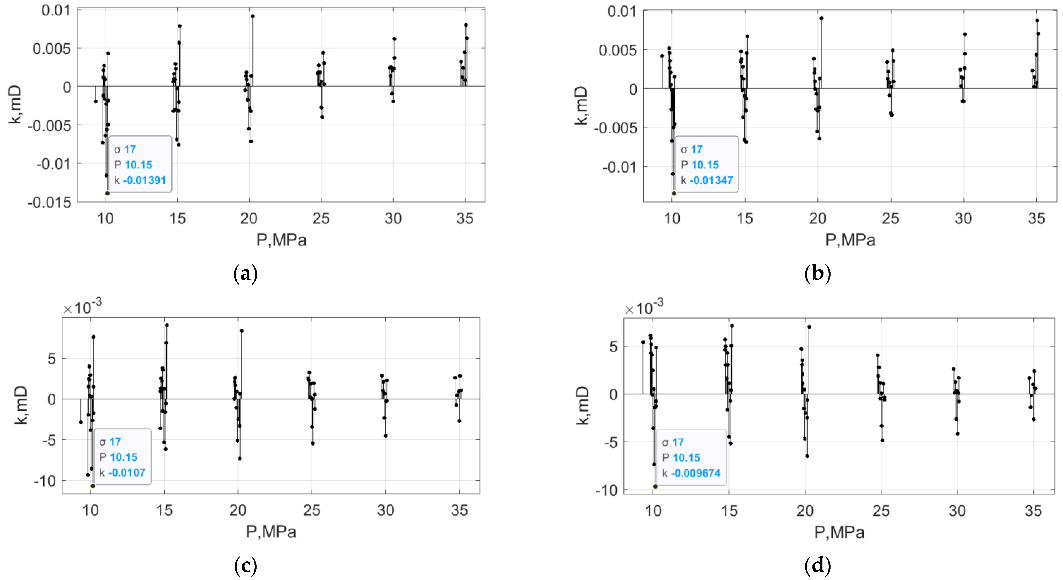
In Figure 7a,b, the distribution range of residual error of the response surface method is from −0.014 to 0.01, and the maximum value of the residual error is 0.01391. Figure 7c,d shows that the distribution interval of the residual error of the 3D surface fitting method is from −0.0107 to 0.01, and the maximum value of the residual error is 0.0107. The distribution interval and maximum value of the residual error of the latter are approximately 0.003 smaller than those of the former, which also indicates that the fitting accuracy of the latter is higher than that of the former.

The 3D surface fitting method performed better than the response surface method in three statistical parameters; although the advantages were not obvious, the superiority was assured. The 3D surface fitting method is of great significance for improving the processing accuracy of experimental data, and lays a good foundation for the research of effective stress law, permeability evolution law, and evaluation of reservoir stress sensitivity.

5. Conclusions

This study analyzed the essence of the cross-plotting and response surface methods. The analysis demonstrated that the preprocessing of the original experimental data and the preset of the function relation might lead to the calculation deviation of ESCP. To avoid calculation deviation and improve the fitting accuracy, a 3D surface fitting method was proposed to calculate the ESCP. The 3D surface fitting method was compared with the cross-plotting and response surface methods by quantitative analysis of the statistical parameters.

(1) Compared with the cross-plotting method, the 3D surface fitting method had obvious advantages: the correlation coefficient was increased by 0.6, and the RMSE and maximum residual error were reduced by nearly three times. The preprocessing of the original experimental data led to the distortion of the calculation results by the cross-plotting method.

(2) The three statistical parameters of the 3D surface fitting method were better than those of the response surface method, and the calculation results were more accurate and reliable.

(3) The power law relationship model between permeability and stress failed to fit the stress-sensitive experimental data of some rock samples, and no basic theoretical support was observed. Therefore, a power law model should be used with caution.

(4) The exponential model of permeability change with stress can be simplified by a theoretical formula, and its mathematical form is simple and widely used.

The key to investigating the effective stress and fluid-structure interaction of porous media lied in the mechanism and functional relationship of the confining pressure and pore fluid pressure on the flow characteristics [30]. When the mechanism of action and function relation were not determined, only the effective stress was insufficient, especially when the effective stress could not be expressed by a simple linear relation.

References

- Terzaghi, K. The shearing resistance of saturated soils and the angle between planes of shear. First Int. Conf. Soil Mech. 1936, 1, 54–59. [Google Scholar]
- Biot, M.A. Theory of Deformation of a Porous Viscoelastic Anisotropic Solid. J. Appl. Phys. 1956, 27, 459–467. [Google Scholar] [CrossRef]
- Biot, M.A.; Willis, D.G. The Elastic Coefficients of the Theory of Consolidation. J. Appl. Mech. Trans. ASME 1957, 24, 594–601. [Google Scholar] [CrossRef]
- Nur, A.; Byerlee, J.D. An Exact Effective Stress Law for Elastic Deformation of Rock with Fluids. J. Geophys. Res. 1971, 76, 6414–6419. [Google Scholar] [CrossRef]
- Yu, B.; Liu, C.; Zhang, D.; Zhao, H.; Li, M.; Liu, Y.; Yu, G.; Li, H. Experimental Study on the Anisotropy of the Effective Stress Coefficient of Sandstone Under True Triaxial Stress. J. Nat. Gas Sci. Eng. 2020, 84, 103651. [Google Scholar] [CrossRef]
- An, C.; Killough, J.; Xia, X. Investigating the Effects of Stress Creep and Effective Stress Coefficient on Stress-Dependent Permeability Measurements of Shale Rock. J. Pet. Sci. Eng. 2021, 198, 108155. [Google Scholar] [CrossRef]
- Ghabezloo, S.; Sulem, J.; Guedon, S.; Martineau, F. Effective stress law for the permeability of a limestone. Int. J. Rock Mech. Min. Sci. 2009, 46, 297–306. [Google Scholar] [CrossRef] [Green Version]
- Meng, F.B.; Li, X.; Baud, P.; Wong, T.F. Bedding Anisotropy and Effective Stress Law for the Permeability and Deformation of Clayey Sandstones. Rock Mech. Rock Eng. 2020, 123, 4707–4729. [Google Scholar] [CrossRef]
- Wang, Y.; Meng, F.; Wang, X.; Baud, P.; Wong, T.-F. Effective Stress Law for the Permeability and Deformation of Four Porous Limestones. J. Geophys. Res.-Solid Earth 2018, 123, 4707–4729. [Google Scholar] [CrossRef]
- Xiao, W.; Bernabe, Y.; Evans, B.; Mok, U.; Zhao, J.; Ren, X.; Chen, M. Klinkenberg Effect and Effective Pressure for Gas Permeability of Tight Sandstones. J. Geophys. Res.-Solid Earth 2019, 124, 1412–1429. [Google Scholar] [CrossRef]
- Berryman, J.G. Effective Stress for Transport Properties of Inhomogeneous Porous Rock. J. Geophys. Res.-Solid Earth 1992, 97, 17409–17424. [Google Scholar] [CrossRef] [Green Version]
- Robin, P.Y.F. Note on Effective Pressure. J. Geophys. Res. 1973, 78, 2434–2437. [Google Scholar] [CrossRef]
- Bernabe, Y. Comparison of The Effective Pressure Law for Permeability and Resistivity Formation Factor in Chelmsford Granite. Pure Appl. Geophys. 1988, 127, 607–625. [Google Scholar] [CrossRef]
- Bernabe, Y. The Effective Pressure Law for Permeability in Chelmsford Granite and Barre Granite. Int. J. Rock Mech. Min. Sci. 1986, 23, 267–275. [Google Scholar] [CrossRef]
- Yang, C.; Liu, J. Petroleum rock mechanics: An area worthy of focus in geo-energy research. Adv. Geo-Energy Res. 2021, 5, 2. [Google Scholar] [CrossRef]
- Wang, F.; Gong, R.; Huang, Z.; Meng, Q.; Zhang, Q.; Zhan, S. Single-phase inflow performance relationship in stress-sensitive reservoirs. Adv. Geo-Energy Res. 2021, 5, 10. [Google Scholar] [CrossRef]
- Walsh, J.B. Effect of Pore Pressure and Confining Pressure on Fracture Permeability. Int. J. Rock Mech. Min. Sci. 1981, 18, 429–435. [Google Scholar] [CrossRef]
- Xiao, W.L. The Study on Non-Linear Effective Stress for Permeability in Low-Permeability Rocks. Ph.D. Thesis, Southwest Petroleum University, Chengdu, China, 2013. [Google Scholar]
- Jones, F.O., Jr. A Laboratory Study of the Effects of Confining Pressure on Fracture Flow and Storage Capacity in Carbonate Rocks. J. Pet. Technol. 1975, 27, 21–27. [Google Scholar] [CrossRef]
- Bernabe, Y. The Effective Pressure Law for Permeability During Pore Pressure and Confining Pressure Cycling of Several Crystalline Rocks. J. Geophys. Res.-Solid Earth Planets 1987, 92, 649–657. [Google Scholar] [CrossRef]
- Xiao, W.L.; Jiang, L.; Li, M.; Zhao, J.Z.; Zheng, L.L.; Li, X.F.; Zhang, Z.P. Effect of Clay Minerals on the Effective Pressure Law in Clay-rich Sandstones. J. Nat. Gas Sci. Eng. 2015, 27, 1242–1251. [Google Scholar] [CrossRef]
- Li, M.; Xiao, W.L.; Bernabe, Y.; Zhao, J.Z. Nonlinear Effective Pressure Law for Permeability. J. Geophys. Res.-Solid Earth 2014, 119, 302–318. [Google Scholar] [CrossRef]
- Dong, J.J.; Hsu, J.Y.; Wu, W.J.; Shimamoto, T.; Hung, J.H.; Yeh, E.C.; Wu, Y.H.; Sone, H. Stress-dependence of the Permeability and Porosity of Sandstone and Shale From TCDP Hole-A. Int. J. Rock Mech. Min. Sci. 2010, 47, 1141–1157. [Google Scholar] [CrossRef]
- Shi, Y.L.; Wang, C.Y. Pore Pressure Generation in Sedimentary Basins: Overloading Versus Aquathermal. J. Geophys. Res.-Solid Earth Planets 1986, 91, 2153–2162. [Google Scholar] [CrossRef]
- David, C.; Wong, T.F.; Zhu, W.L.; Zhang, J.X. Laboratory Measurement of Compaction-induced Permeability Change in Porous Rocks: Implications for the Generation and Maintenance of Pore Pressure Excess in the Crust. Pure Appl. Geophys. 1994, 143, 425–456. [Google Scholar] [CrossRef]
- Yin, S.X.; Wang, S.X. Rock permeability at different scales and the relationship between stress and its mechanism. Sci. CHINA (SERIES D) 2006, 5, 472–480. [Google Scholar]
- Qiao, L.P.; Wang, Z.C.; LI, S.C. Effective Stress Law for Permeability of Tight Gas Reservoir Sandstone. Chin. J. Rock Mech. Eng. 2011, 30, 1422–1427. [Google Scholar]
- Zhao, J.; Xiao, W.; Li, M.; Xiang, Z.; Li, L.; Wang, J. The Effective Pressure Law for Permeability of Clay-Rich Sandstones. Pet. Sci. 2011, 8, 194–199. [Google Scholar] [CrossRef] [Green Version]
- McKee, C.R.; Bumb, A.C.; Koenig, R.A. Stress-dependent Permeability and Porosity of Coal and Other Geologic Formations. SPE Form. Eval. 1988, 3, 81–91. [Google Scholar] [CrossRef]
- Zhang, T.; Li, Z.; Adenutsi, C.D. A new model for calculating permeability of natural fractures in dual-porosity reservoir. Adv. Geo-Energy Res. 2017, 1, 7. [Google Scholar] [CrossRef] [Green Version]
- Reyes, L.; Osisanya, S.O. Empirical Correlation of Effective Stress Dependent Shale Rock Properties. J. Can. Pet. Technol. 2002, 41, 47–53. [Google Scholar] [CrossRef]
- Chalmers, G.R.L.; Ross, D.J.K.; Bustin, R.M. Geological Controls on Matrix Permeability of Devonian Gas Shales in the Horn River and Liard Basins, Northeastern British Columbia, Canada. Int. J. Coal Geol. 2012, 103, 120–131. [Google Scholar] [CrossRef]
- Dou, H.G.; Zhang, H.J.; Yao, S.L.; Zhu, D.; Sun, T.; Ma, S.Y.; Wang, X.L. Measurement and evaluation of the stress sensitivity in tight reservoirs. Pet. Explor. Dev. 2016, 43, 1022–1028. [Google Scholar] [CrossRef]
- Lu, R.B.; Hu, L.; Wang, W.J.; Yang, L.; Zhang, Q. Stress Sensitivity Characterization and Field Application in High Temperature-Pressure Gas Reservoir. Spec. Oil Gas Reserv. 2020, 27, 108–113. [Google Scholar]
- Zheng, Y.X.; Liu, J.J.; Liu, Y.C.; Shi, D.; Zhang, B.H. Experimental Investigation on the Stress-Dependent Permeability of Intact and Fractured Shale. Geofluids 2020, 2020, 8897911. [Google Scholar] [CrossRef]
Figure 1.
Fitting curves of experimental data of rock samples 1 and 2. (a) Sample 1 was fitted by a quadratic polynomial; (b) sample 1 was fitted by the exponential model; (c) sample 2 was fitted by a quadratic polynomial; (d) sample 2 was fitted by the exponential model.
Figure 2.
Experimental data of rock sample D13−4 was fitted by a quadratic polynomial. (a) Set the ESCP as 1; (b) set the ESCP as 0.3537.
Figure 3.
Longitudinal section of 3D fitting surface for the experimental data of rock sample D15−2. (a) Sample D15−2 was fitted by the exponential model (ESCP was set as 0.7978 calculated by the 3D surface fitting method); (b) sample D15−2 was fitted by the exponential model (ESCP was set as 0.6479 calculated by the response surface method).
Figure 4.
Residual error distribution diagram (rock sample 1). (a) The cross-plotting method (quadratic polynomial fitting rock sample 1); (b) the cross-plotting method (exponential fitting rock sample 1); (c) the 3D surface fitting method (quadratic polynomial fitting rock sample 1); (d) the 3D surface fitting method (exponential fitting rock sample 1).
Figure 5.
Residual error distribution diagram (rock sample 2). (a) The cross-plotting method (quadratic polynomial fitting rock sample 2); (b) the cross-plotting method (exponential fitting rock sample 2); (c) the 3D surface fitting method (quadratic polynomial fitting rock sample 2); (d) the 3D surface fitting method (exponential fitting rock sample 2).
Figure 6.
Residual error distribution diagram (rock sample D13−4). (a) The response surface method (quadratic polynomial fitting rock sample D13−4); (b) the response surface method (exponential fitting rock sample D13−4); (c) the 3D surface fitting method (quadratic polynomial fitting rock sample D13−4); (d) the 3D surface fitting method (exponential fitting rock sample D13−4).
Figure 7.
Residual error distribution diagram (rock sample D15−2). (a) The cross-plotting method (quadratic polynomial fitting rock sample D15−2); (b) the cross-plotting method (exponential fitting rock sample D15−2); (c) the 3D surface fitting method (quadratic polynomial fitting rock sample D15−2); (d) the 3D surface fitting method (exponential fitting rock sample D15−2).