
Graph Modeling for Efficient Retrieval of Power Network Model Change History


1
Faculty of Technical Sciences, Department of Power, Electronic and Telecommunication Engineering, University of Novi Sad, Trg D. Obradovića 6, Novi Sad 21000, Serbia
2
Faculty of Technical Sciences, Department of Computing and Control Engineering, University of Novi Sad, Trg D. Obradovića 6, Novi Sad 21000, Serbia
*
Author to whom correspondence should be addressed.
Energies 2021, 14(24), 8351; https://doi.org/10.3390/en14248351
Submission received: 30 October 2021
/
Revised: 6 December 2021
/
Accepted: 8 December 2021
/
Published: 11 December 2021
(This article belongs to the Topic Innovative Techniques for Smart Grids)
Abstract
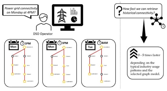
:Power grids are constantly evolving, and data changes are increasing. Operational technology (OT) is controlled by IT technologies in smart grids, where changes in the physical world impose changes in the software data model, as well as the continuous generation of data points, resulting in time series datasets. The increased need for processing large amounts of data combined with requirements to maintain and increase overall performances has created a significant challenge for traditional database solutions and relational database models. The main idea of this paper was to find and propose a graph model that will allow the retrieval of historical connectivity in a reduced time complexity. Furthermore, the research question was addressed by evaluating three different approaches where the results provide a foundation for the proposed design guidelines related to optimizing graph-based databases for a modern smart grid system. The results of the experiments demonstrated reduced time complexities from 3 to 5 times depending on the typical industry usage patterns and the selected graph model. This suggests that the design decision may severely affect the outcome for given smart grid use cases when using historical features in OT technologies. Therefore, the main contribution of the research is the proposed guidelines on how to design an optimal graph model that satisfies the described smart grid requirements.
1. Introduction
Power network grids (the grids herein) were designed in the previous century, but the requirements and context of modern cities have forced the grid to evolve, rendering current grids obsolete. Connectivity in the grids can vary as a consequence of: (1) changes in the state of its elements such as switching the equipment on and off, or (2) physical changes to the grid’s topology such as extending the feeders to new parts of the city or replacing existing equipment. We focused on the first scenario, while the second scenario introduces a much lower rate of changes in the equivalent period. If the grid is in an area often exposed to hazards or climate disaster—connectivity will be more affected. In usual scenarios, there are about a hundred changes during a day, and during storms (e.g., storm mode), there are about several thousand. Distribution System Operators (DSO) make various analyses as they must have insight into the connectivity of the whole network, both in real-time and to keep a history for training purposes and post-accident analyses. As operational technology (OT) is controlled by IT technologies in smart grids, changes in the physical world impose changes in the software data model. Processing large amounts of data, while maintaining performances for a real-time decision-making software system, creates a problem for traditional database solutions and relational database models.
One of the main advantages of graph databases in smart grids over relational databases and NoSQL stores is performance, as they are optimized for the graph data models. Graph databases are typically thousands of times more powerful than traditional databases in terms of indexing, computing power, storage, and querying. In relational databases, performances on data relations decrease as the dataset grows. Smart grid data increase on a daily basis, so graph databases could be a better solution, as the performance remains relatively constant. In addition, smart grid models are very complex and change frequently. This can be a problem as relational databases require a comprehensive data model up front. Moreover, graph databases are inherently flexible, because graphs can be extended with new vertices and new edge types almost effortlessly [1].
DSO data can be generated by various equipment and stored in different formats:
- Raw waveforms (voltage and currents) sampled at relatively high sampling frequencies
- Pre-processed waveforms (e.g., RMS) typically sampled at low sampling frequencies.
- Status variables (e.g., if a relay is opened or closed) typically sampled at low sampling frequencies.
Here, we consider historical data of status variables, which are part of the Supervisory Control and Data Acquisition (SCADA) systems [2]. The historical database is an important component in typical SCADA architecture, and it is used to store all data collected by the system. The historical database stores a significant quantity of data, as it stores thousands of alarms, statuses of digital variables, and nominal values of analog variables [3]. In this paper, the focus was on digital values as the sample rate is substantial when compared to the rate of static data changes. A digital value can represent the status of circuit breakers, trip relays, fuses, switches, and other grid equipment. Therefore, we are dealing with partially evolved dynamic graphs [4] as we are considering just attribute evolution—dynamic graph changes represented by the actions: add attribute value, remove attribute value, or update attribute value. In this scenario, remove attribute is not allowed, as the status can be either OPEN or CLOSED and it cannot be omitted.
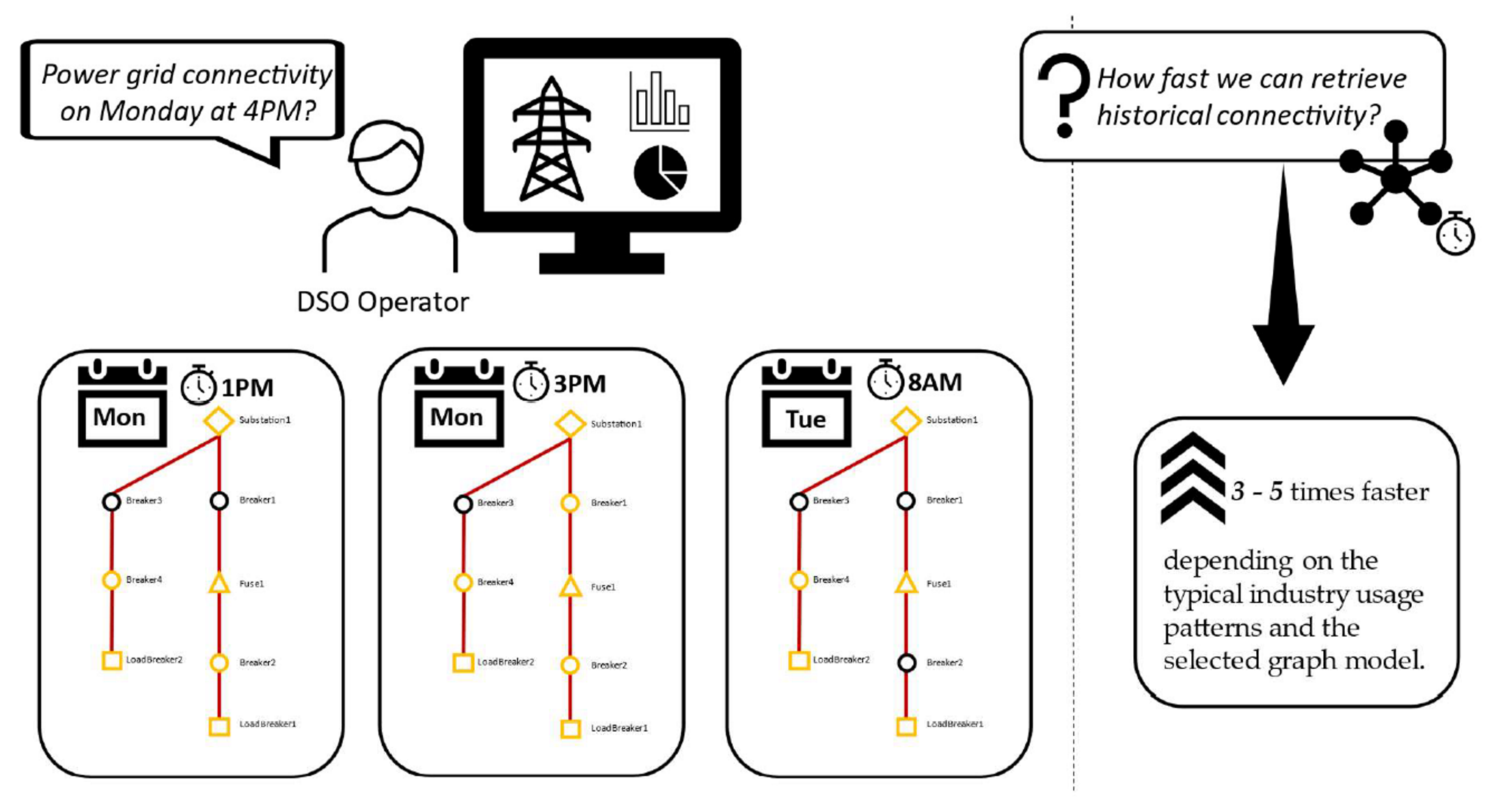
The main idea is to provide a full recreation of the network topology representing the grid at an arbitrary time in history. Usually, time series databases are designed to provide a fast read and write by element, making it difficult to query a whole set or subset of graph elements in a particular period. Therefore, the research question of this paper is what is the most efficient graph database model to provide an efficient write per graph element while providing an efficient graph or subgraph scan for different time points? This is a slightly different problem in comparison to the other problems focused on in historical databases presented in related works. The main issue in replaying the historical sequence of network topology changes or retrieving a graph connectivity in an arbitrary historical point is that we cannot query data samples by datetime unless we search for historical value in each element of the graph model. The time complexity of such an algorithm would be quadratic (O(n2)), rendering such an approach inapplicable for large data models and real-time characteristics of smart grids. The large data models are a consequence of the dynamics of data—some statuses can stay unchanged in history for a long time, while other statuses might change. The result is to have slowly changing values correlated with different values in the same timeline (Figure 1). The properties of smart grid data changes described introduce difficulties in designing an efficient historical data model. For instance, if we look at just four vertices, and its few changes for one day (Figure 1)—all vertices have an initial value of status, and every next vertex is a change during time. Assume that we want to see how those vertices were connected in any moment in time—in Figure 1, this moment is tx.
If we simply go through vertices and search for that exact date (tx), our query will return an empty value. The correct returned value should be BRE1:OPENED—DIS1: CLOSED—BRE2:OPENED—DIS2:OPENED. Having an efficient solution for querying described dynamic graphs in time would provide a usable feature for DSOs as it would enable the analysis of events that happened in the past.
In this paper, we focused on finding and proposing a graph model that will allow the retrieval of historical connectivity in a reduced time complexity. As with modeling any solution, there is no one approach that is the optimal in all circumstances, even though we are focused on smart grid use cases. Therefore, we investigated three different approaches based on the graph theory and existing research in the area of graph databases. The three approaches were applied to modeling the same instance of a real power distribution grid network model resulting in three referent test sets. Test sets were built for a commercially available graph database management system (Neo4j) that was used for running the experiments. The experiments revealed the performances of different queries that correspond to the described smart grid use cases. Along the proposed graph models optimized for reduced time complexity when retrieving the historical graph connectivity, the main contribution of this paper is the resulting guideline that elaborates when to use which graph model type based on the smart grid use cases and patterns of database usage. In Section 2, we describe related works. Section 3 describes the methodology and specific approaches that have been chosen and how they have been implemented. Section 4 presents the experiments and provides the results, while Section 5 is dedicated to the evaluation of the results and discussion. Finally, Section 6 summarizes the main points and outlines further research steps.
2. Related Works
Many tools and libraries have been developed for social network analysis, but they are all mainly focused on examining static network snapshots. Not much work has been performed on the analysis of temporal or evolving graphs and neither one of the graph data management systems handles optimizing snapshot retrieval queries over historical graphs, or on supporting temporal analysis of large networks [5].
The focus of the research concerning evolving graphs has been on efficiently storing and retrieving graph snapshots. This is the predominantly used approach for graph analysis due to its accessibility. A snapshot method captures a sequence of static graphs from a temporal graph; thus, existing graph algorithms can be directly applied to each static graph [6]. The authors’ main idea in Ref. [7] was to store the historical trace of the network on a disk, and to load the required graphs on-demand in memory. They used a collection of graph historical snapshots, one corresponding to each time instance. For large temporal graphs, there are studies on graph partition [8]. They store individual snapshots of a single graph on different computers. Semertzidis and Pitoura [9] discussed an alternative approach for storing time-varying networks using a hierarchical time index to support snapshots with different granularity and presented historical graph queries. Cattuto et al. [10] presented the historical graph stored as a sequence of graph snapshots, where vertices and edges are associated with time intervals. In Ref. [11], graph mining algorithms were provided that assume a static underlying graph.
The time-versioning process has been proven by various authors. The problem that they introduce is an increase in complexity of the graph structure, as well as the complexity of the queries, which leads to a reduction in performance, scalability, and maintainability. Castelltort and Laurent [12] created a meta-graph, which chains history in a linked list. The history of edges is considered with two approaches—single and multi-edge. This adds more complexity, due to the increased number of checks in each query, which leads to poor performance for deep history. There is a different approach for creating a meta-graph [13], which is based on modeling differences between versions as graphs. The biggest problem, from a performance standpoint, is graphs that have a lot of incoming/outgoing edges.
Maduako et al. [14] made a time-tree for the timeline, and each vertex was connected to a leaf in that tree according to the time when it is created. As we are dealing with a complete graph recreation problem, where the solution gives insight to the grid manager into the historical network state from moment x to moment y, and we want to have information about how elements in the grid were connected in each moment, these approaches would not provide the required results.
Nowadays, graph databases have been used for a wide variety of power system analyses, such as power flow calculation, topology analysis, state estimation [15], and real-time EMS framework [16]. In Ref. [17], traditional relational databases (PostgreSQL) were compared with graph databases (Neo4j) in the analysis of power grid data. With experiments, they demonstrated a better performance of topology modeling and analysis using graph databases. However, they did not cover historical data. Liu et al. [16] proposed an EMS real-time analysis framework for an evolving graph-based power system.
Even though extensive research in the area of modeling the history within graph databases exists, to the best of the authors knowledge, no work has provided an experimentally confirmed comparison of different approaches retrieving the historical connectedness of the power network graph models. With the aim to provide the best approach to reduce the time complexity of retrieving the connectivity in arbitrary historical points, this paper proposes clear guidelines on what graph model type to use based on the smart grid use cases and patterns of database usage.
3. Methodology
For a vertex, the number of head ends adjacent to a vertex is called the indegree of the vertex and the number of tail ends adjacent to a vertex is its outdegree.
Definition 1 (Graph).
A graph G is given by a pair (V, E) where V stands for a set of vertices and E stands for a set of edges with E⊆ (V × V).
Definition 2.
For G = (V, A) and v∈ V, the indegree of v is denoted as deg-(v) and its outdegree is denoted as deg + (v).
Definition 3.
Inset, I(v) = {x | (x, v)∈ E}, is the set of all vertices that represent head ends adjacent to a vertex.
Definition 4.
Outset, O(v) = {x | (v, x)∈ E}, is the set of all vertices that represent tail ends adjacent to a vertex.
Data structures that can preserve a graph’s history are called temporal, evolving, or time-varying graphs [18]. There are several ways of modeling formally discrete temporal graphs. One is to consider an underlying static graph and assign a set of natural numbers, called a label, to every edge. Another one is to view a temporal graph as a sequence of static graphs, as used by the authors in Ref. [6]. Finally, it is useful to expand the whole temporal graph in time and obtain an equivalent static graph without losing any information. A common approach to solving this problem is to first express the given temporal graph as a static graph and then try to apply or adjust one of the existing tools that works on static graphs.
The research methodology (Figure 2) consisted of five steps:
- Formulating the research question: the approach started from the transfer of knowledge from industry to academia. The issue of time complexity in retrieving the historical graph connectivity led to the research of the available literature, as described in Section 2. Once the scientific gap emerged, the research question was formulated: how to provide a full recreation of graph connectivity representing the grid at any time in history consisting of frequent topology changes.
- Hypothesis definition: we needed to define a hypothesis that would address the research question, provide the basis for the advancement of the scientific field, and define supporting claims that can be verified experimentally. The main hypothesis in this paper is: if we define graph models where historical values are connected to the power grid elements in the same graph, the time complexity will be reduced for retrieving graph connectivity in any given moment in history, while the space complexity will not contain any data duplication.
- Experimental validation of hypothesis claims: in order to ensure a valid context for experiments, we relied on a model of a real distribution power grid, as described in Section 4.2. Using the same real model, we created test data for different graph models where each graph model has been created to support a hypothesis based on graph theory and the research of related works. In essence, we created an exporter from the existing SQL-based model by relying on the Common Information Model (CIM) standard. Then, we imported the same model to the graph database but in three different ways, to reflect each of the proposed approaches described in Section 3.1, Section 3.2 and Section 3.3. With ensured valid test data samples, we designed three experiments to address all the inputs defined by use cases that we are focusing on in smart grid problems. The inputs needed to analyze the overall solution are: a typical random write to the graph (see Section 4.4), a typical random read of node values from the graph (see Section 4.3), and retrieving graphs and subgraphs from any moment in history (see Section 4.5).
- Result analysis and presentation: after collecting the measurements from experiments, we performed statistical analysis of the data, and we decided to present the results in tabular form with the given standard deviation to outline how close to the mean were our averages. Moreover, for easer discussion, we extracted graphs to visually present the information to the reader.
- Conclusion: as described in Section 5, we used typical use cases and usage patterns that can be found in industry and applied them in the context of experimental results. Each typical use case was defined as a scenario, and our discussion around scenarios provides a guideline when each of the proposed graph models would make the most benefit considering the main hypothesis. These guidelines confirm supporting claims of the hypothesis and provide the innovation of this paper as they can be used by anyone interested in our research question.
The following sections elaborate the three most representative approaches.
3.1. The First Approach
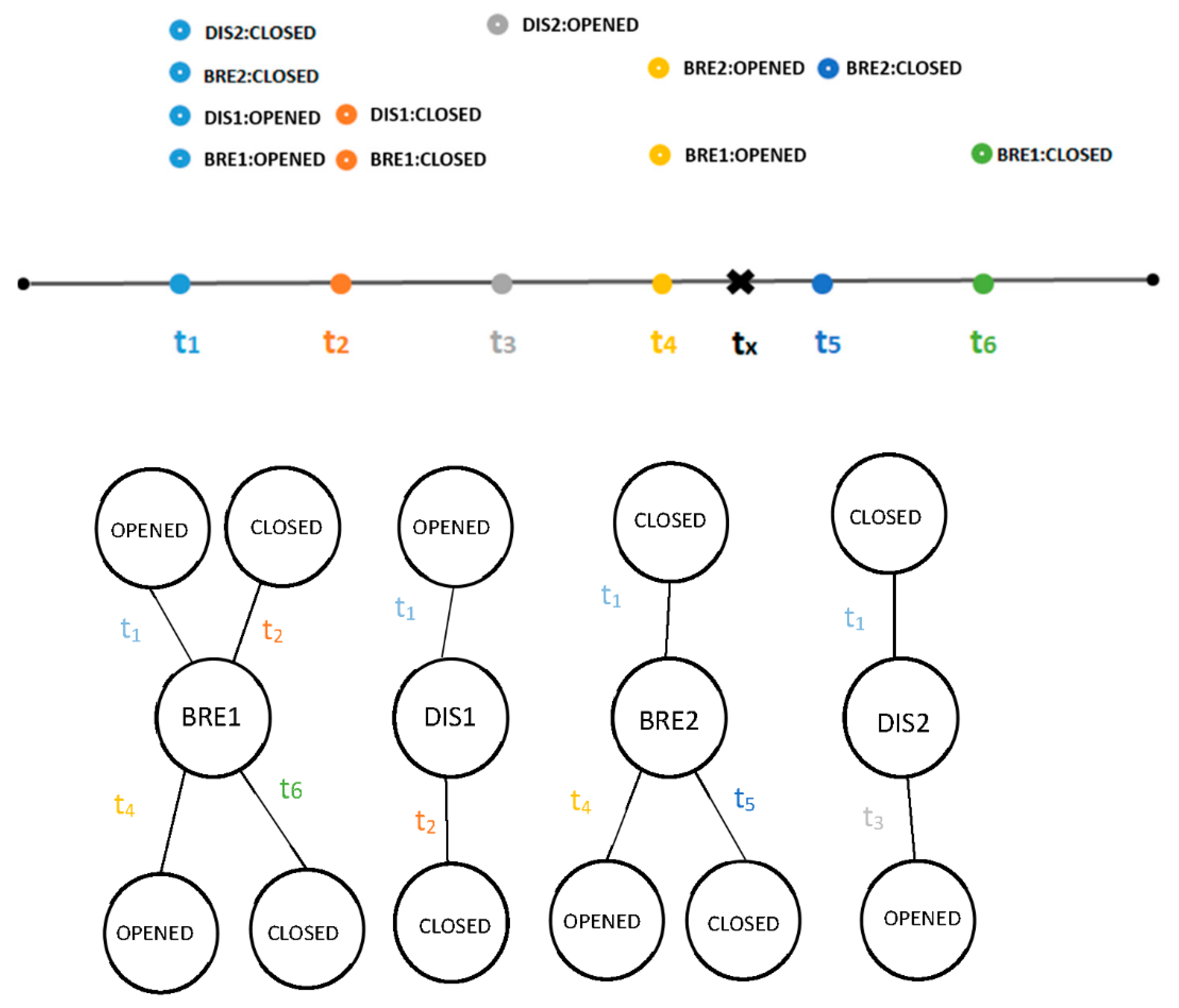
The first approach implies creating a new vertex for every change in the network model and adding reference to the previous change. A linked list is generated and expanded by each new value. The formula below represents how a new vertex is added:
where v represents a vertex and e represents an edge.
For each new vertex, we obtain all vertices with the same id, and to determine which one is the most recent one, we find one without an edge with id next.
3.2. The Second Approach
With the second approach, as proposed by the authors in Ref. [19], we are also creating a new vertex for every change. However, we are not linking them; instead, we are connecting all outset and inset vertices with a new value. The formula below shows how a new vertex is added:
where v represents a vertex, o represents outset, i represents inset, and e represents an edge.
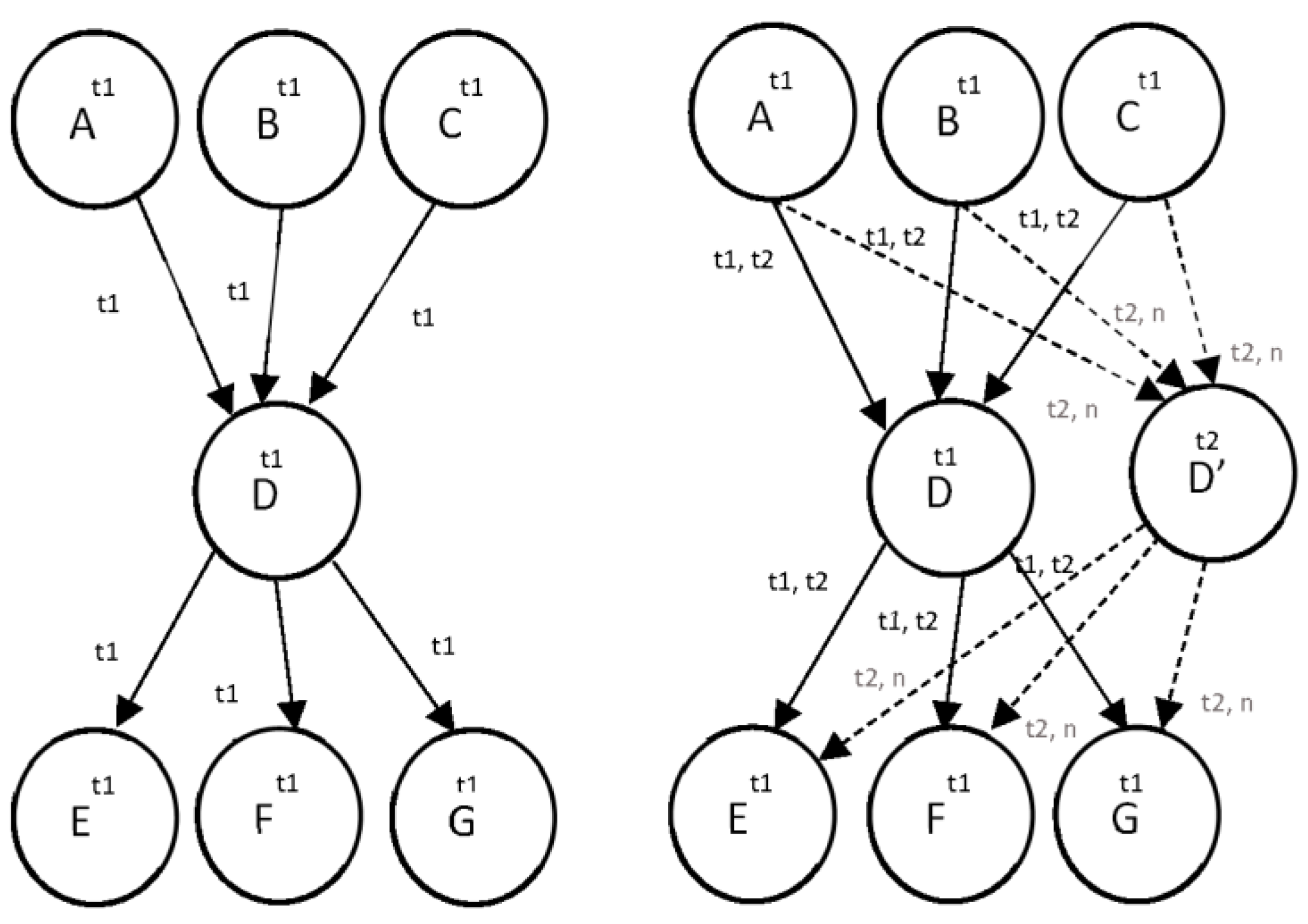
Figure 5 shows one element D added in time t1. For adding a new vertex D’ with a new timestamp t2, it needs to inherit all currently valid edges. Each new vertex and edge will be expanded with a created attribute, as well as old ones with the addition of an expired attribute.
Copying a vertex requires copying all live edges, which removes a limitation of having a constant number of graph operations. Figure 6 shows a BDA for adding a new status value. Beyond adding a new vertex, we are adding an additional property with a timestamp of creation. Furthermore, we are adding an expired attribute with the same timestamp to the previous vertex, as its value is valid until the new value has been created.
3.3. The Third Approach
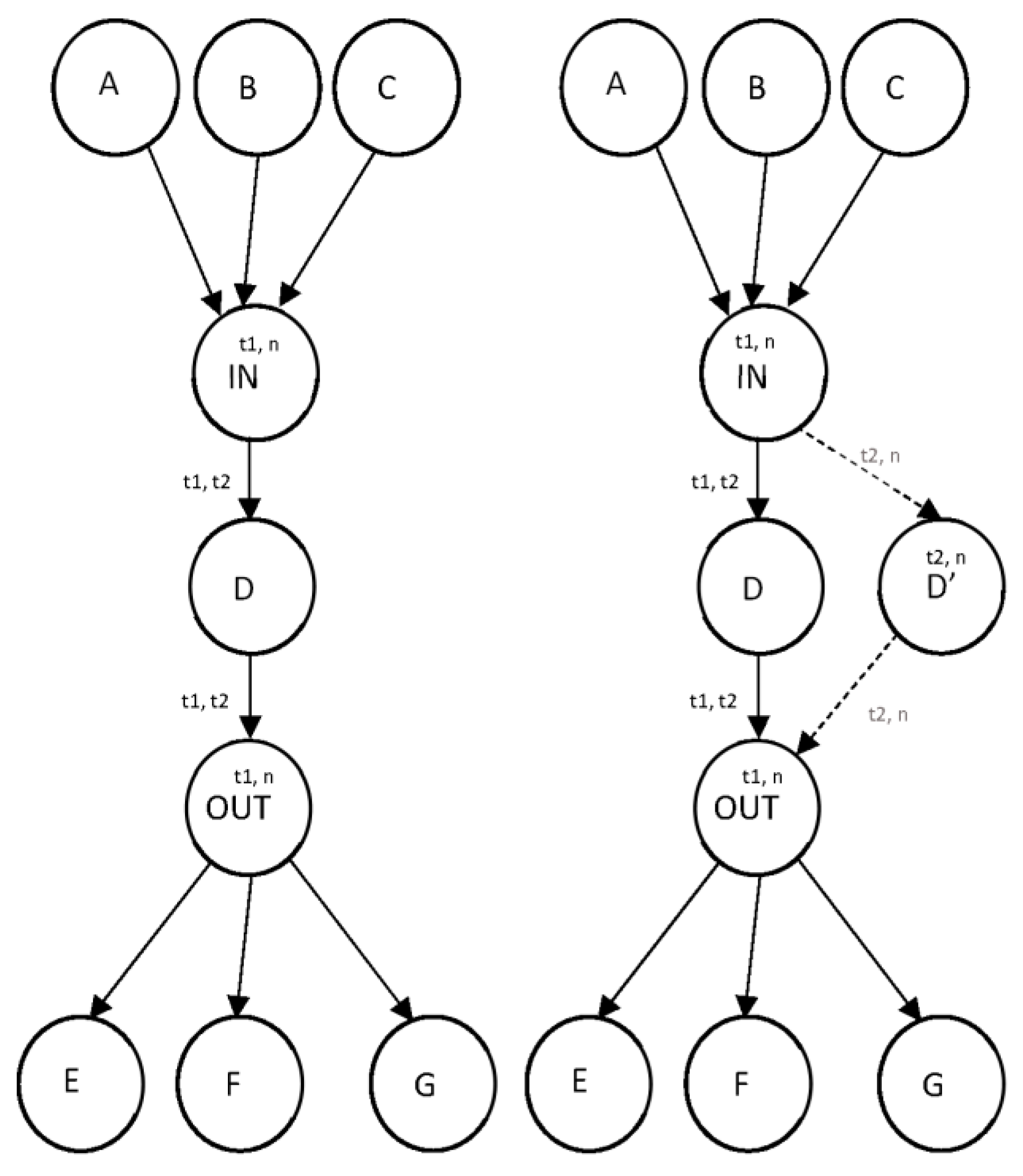
With the previous approach, there is a deficiency in the case where the vertices have a lot of incoming and/or outgoing changes. When a new vertex is being added, all those edges need to be copied to the new vertex (Figure 7). Therefore, this approach is an extension of the second one—each vertex implies adding two additional ones that act as a proxy for all vertices created prior to the actual vertex.
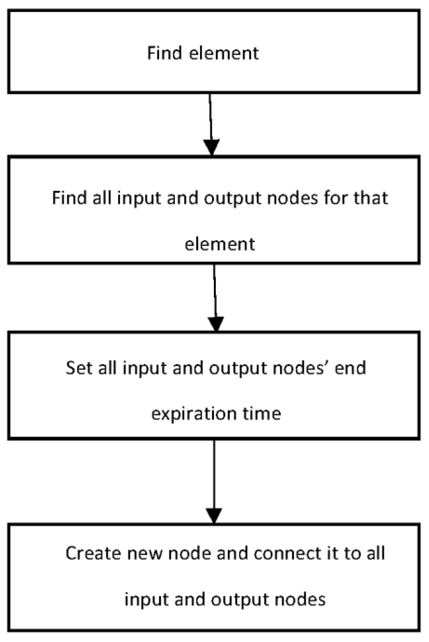
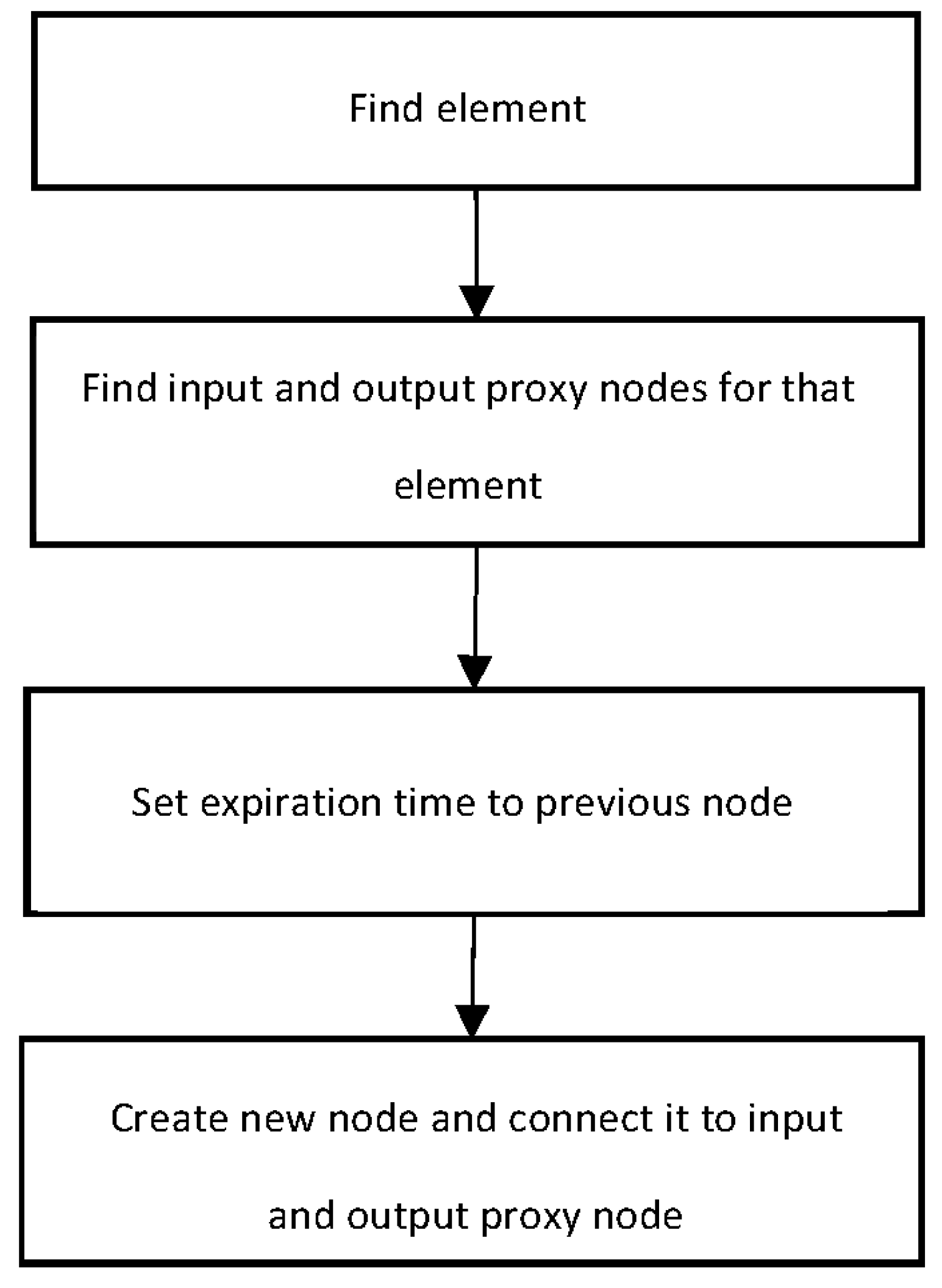
The main idea behind this is to add one additional vertex for all edges with outgoing vertices and one vertex for all edges with incoming changes. The additional vertices will provide connectivity within all vertices as before, but they will reduce the number of edges (Figure 7). Still, we are adding additional properties created and expired, but now onto proxies besides vertices and edges. A constant number of graph operations and additional space per modification are achieved. Figure 8 shows a block diagram algorithm (BDA) for adding a new status value.
4. Experiments
This section presents the experimental results, with the intention of evaluating and analyzing each approach using the same test environment and test data. Three different experiments were focused on in evaluating different operations, so the discussion section elaborates the advantages and disadvantages of proposed approaches based on the relevant data.
4.1. Test Environment
Table 1 shows physical machine properties for the testing environment.
The physical machine hosted a virtual machine using the Hyper-V hypervisor and Microsoft Windows Server OS with Neo4j [20] installed and used as a graph database management system.
4.2. Test Data
The test dataset represents a real network data model (Network Model) of a European-based DSO company. The data are defined in an industry standard model CIM [21,22] that defines how objects and edges between power system resources are represented. The network model describes the static elements of the electrical distribution system. Therefore, it describes the network connectivity along with other power system resource properties needed for arbitrary power function. Table 2 shows the main characteristics of a distribution network used as a test set.
Each vertex represents a power resource element of the network (breaker, transformer, fuse…) and each edge between them represents the connectivity between them.
For the described data model, we have used an industry-proven field data simulator for generating dynamic data, with the characteristics shown in Table 3. This paper takes into account just discrete value changes, and for now, analog value changes are not part of the research. The simulator generates data in two modes—in normal mode when there are about a hundred changes during the day, and in storm mode when there are a couple of thousand changes. Of course, the number of changes in both modes differ from network to network—if we are dealing with a network where the equipment is not in a good state, during storm mode, there will be more outages and vice versa. Hence, we are assuming that the network is in a good state.
In the following sections, three experiments are described—Standard queries, Update, and State recreation. The execution time for the selected queries is measured in Standard queries, while the time for updating new values in the database is measured in Update. In the last one, a focus is set on execution time for retrieving elements and their connection for a given moment in history.
4.3. Experiment 1—Standard Queries
First, we measured execution time for three different queries without any history. Then, we measured execution time for the same queries in near (couple of days—10 changes per element) and far history (couple of years—390 changes per element). The following queries were used:
- Get hierarchy to substation by breaker ID (query 1). Hierarchy assumes all elements that are connected from the breaker vertex to the substation vertex (subgraph).
- Fetch all elements from a particular feeder (query 2). For a given feeder, a query returns all breakers, fuses, disconnectors, and any other equipment.
- Fetch all devices where the device name contains a given string parameter (query 3).
Time execution for typical queries for the first approach is shown in Table 4, for the second approach in Table 5, and for the third in Table 6. Each table shows the average time that was needed for executing a different query for each approach, as well as the relative standard deviation (CV) with eliminated outliers.
4.4. Experiment 2—Update
The goal of the second experiment was to show a comparison of the proposed approaches for updating values. In total, 78,573 update operations were performed per approach. Table 7 shows the average time that was needed for executing update operations for each approach.
As expected, the relative standard deviation was higher in this experiment compared to the first one, as in this one, the uncertainty was naturally assumed as each update operation may end up in a different part of the graph with different complexity and historical depth. Figure 12 shows the execution time of an update operation for all three approaches. In the first approach, we need to find the element that needs to change—and find the one with the latest date time. However, in the other two approaches, it depends on how much outgoing and ingoing changes that vertex contains, as the new vertex needs to be connected to all of them. It could be the case that the vertex does not have outgoing or ingoing vertices at all, or that it has only a few or even several hundred. Depending on vertex connectivity, the execution time can vary from a few milliseconds to more than a second.
4.5. Experiment 3—State Recreation
The third experiment focused on testing how fast a state of the network can be obtained for a given moment in history. The state of the network represents how elements of the network are connected—and what their statuses are. The experiment included all three scenarios. Figure 13, Figure 14 and Figure 15 show part of the network on which queries were executed. The legend defines symbols and their meanings. Each vertex and edge have a pair of timestamps next to them. The pair consists of creation and expiration timestamps. Edges that correspond to t2 are marked with a red line, while corresponding vertices are marked with a yellow one. Table 8, Table 9 and Table 10 show the execution time for the state recreation function using 1, 2, and 10 edges, respectively. Experiment three aimed to display a relationship between the size of the network and the execution time for the state recreate function.
4.5.1. The First Approach
Figure 13 represents a part of the network, and the elements that should be retrieved for t = t2. In this approach, each time we are executing the state recreation function, we need to find the element that has a required time that is between the created and expired timestamp attribute. For instance, if connectivity for t = t2 (Figure 13) is needed, the query would start from Substation1 and Breaker1. Breaker1 has two vertices (two history points), and for t2, the rightmost vertex is marked yellow. However, if we just obtain that vertex, we will not have information about the Breaker1 edges. Therefore, within the query, it is also required to retrieve the one that has an edge with the next vertex (in this case, Fuse1). There are four history points in the case of Fuse1, while the one with an interval that corresponds to t2 is needed (the leftmost one). In addition, the query needs to include Fuse1 with an edge to Breaker2 (which is the same as the previous one in this case).
4.5.2. The Second Approach
Figure 14 represents the part of the network outlining which elements should retrieve the function for t = t2. Queries that include history are the same as the ones without, with just one additional check—whether the timestamp is between created and expired.
First, the query finds substation1 with created time t1, where the expired time is not set, which means there is only one history point for substation1. There are two edges between Substation1 and Breaker1—one is for the time range t1–t2 and the other is for t2–present. We take the second one, as we need the history point t2. Next, four edges exist between Breaker1 and Fuse1; as t2 goes into the range t2–t3, we take the first edge. Only one edge exists between Fuse1 and Breaker2 and t2 is within that range. The same is applicable for the edge between Breaker2 and LoadBreaker1. The same pattern is used for another branch.
4.5.3. The Third Approach
Figure 15 represents a part of the network outlining which elements should retrieve the function for t = t2, with grey circles presenting IN/OUT vertices. Each pair of element and its IN and OUT vertex are altogether grouped by dotted line. Basically, the logic here is the same as in the second approach, only with one extension—there is one additional step in all queries because of the IN and OUT vertices. The query starts from substation1 with created time t1, and expired time without a value, which means there is only one history point for substation1. To find the connectivity between Substation1 and Breaker1, the OUT vertex for Substation1 is needed. From this vertex, there are two edges to the Breaker1_IN vertex—one is for the time range t1–t2 and the other is for t2–today. The search would continue from the second one, as we need history point t2.
5. Discussion
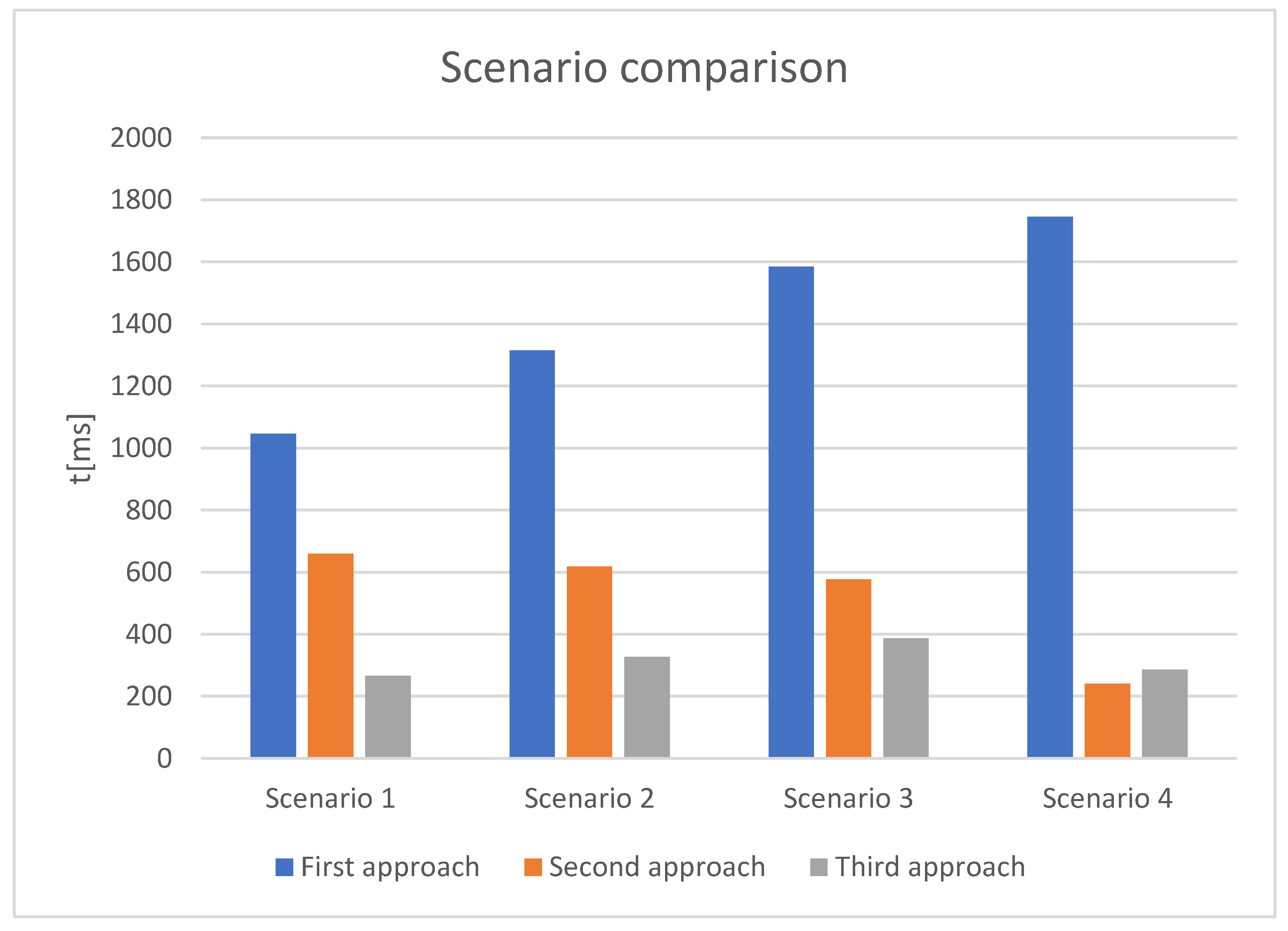
The aim of the experiments was to demonstrate how different approaches affect the performances of queries, insert, and state recreate operations. As expected, each approach has its advantages. Therefore, when designing a final solution, it is important to have reliable data that help guide a design decision. Consequently, we compared all three approaches by introducing hypothetical use cases based on practical experience from the industry. The scenarios were created by using the anticipated percentage of operation executions depending on the usage patterns required by the typical DSOs. We identified four representative scenarios with ratios defined in Table 11. The percentage in a scenario refers to the number of executed operations, not the time needed for the execution.
Figure 16 represents the comparison between all approaches for four representative use cases. The ordinate displays different scenarios defined within Table 11. Each scenario assumes a different percentage in usage patterns for querying, insertion, or using the state recreation function. The results of scenarios are summarized in Figure 15, where average values of samples were used for simulating the outcomes of the scenario. In this way, we can analyze how different approaches would affect performances of the overall solution based on the common usage patterns.
In the first scenario, the first approach is slower than the second one by 37%, and the second one is slower than the third one by 59.7%. In the second scenario, the first approach is slower than the second one by 53%, and the second one is slower than the third one by 47.2%. In the third scenario, the first approach is slower than the second one by 63.6%, and the second one is slower than the third one by 32.86%. In the fourth scenario, the first approach is slower than the second one by 81%, while the second one is faster than the third one by 18.51%.
As it strongly suggests, the first approach should be avoided in similar problems as ours. In the majority of cases, the third approach is the best design decision and the one we recommend if usage patterns are unknown. The second approach might be an optimization only for query-intensive scenarios, implying that write operations are up to 5% of the total number of executed operations. In addition, considering Figure 8, Figure 9 and Figure 10, it is worth noting that queries provide quicker responses when the second approach is used. Therefore, considering the query-intensive nature of some usage patterns, the second approach would be our recommendation.
6. Conclusions
DSOs need to be able to gather, analyze, and transform data coming from different devices in a distribution network. We considered some of the most common queries that would be of interest for DSOs’ business needs.
Power grid topology varies due to state changes in power system resources. Those changes can be the consequence of a regular operation of the grid such as switching the equipment on and off, or a physical change of the grid’s topology such as extending or replacing equipment due to the change in power distribution infrastructure driven by evolving smart cities.
The research question addressed in this paper is how to provide a full recreation of graph connectivity representing the grid at any time in history consisting of frequent topology changes.
Three different approaches were analyzed in order to satisfy seemingly opposite requirements: to provide an efficient write per graph element while providing an efficient graph or subgraph scan at different historical time points.
The results enabled us to provide clear guidelines on which approach to take when designing a solution to address our research question. However, it is worth noting that this paper considered only static changes that reflect physical changes on the grid. Real-time changes initiated by the regular network operations should be additionally analyzed if such a solution is needed. In such a solution, there would be many more changes that would impact the overall performance and would make the solution more write-intensive, which would eliminate the second approach as a possible optimization. Consequently, future work will try to address dynamic changes as well, aiming to combine the first and the third approach using advanced algorithms relying on parallel data processing. The temporal graph database is a useful means for pattern recognition, especially in cybersecurity problems. As smart grids are critical systems, cybersecurity is essential for such systems, and graph models such as those presented in this paper can be a good approach for addressing cybersecurity challenges. Therefore, applying our research findings in smart grid cybersecurity will be a subject for future work as graph models may optimize pattern recognition.
Author Contributions
Conceptualization, I.D., N.D. and A.E.; methodology, I.D.; software, I.D.; validation, N.D. and A.E.; investigation, I.D.; resources, J.M., I.D. and N.D.; data curation, I.D. and A.E.; writing—original draft preparation, I.D. and N.D.; writing—review and editing, A.E. and J.M.; visualization, I.D. and J.M.; supervision, A.E. and J.M. All authors have read and agreed to the published version of the manuscript.
Funding
The authors express their sincere gratitude to the Ministry of Education, Science and Technological Development of the Republic of Serbia for supporting this work within project III-42004.
Institutional Review Board Statement
Not applicable.
Informed Consent Statement
Not applicable.
Data Availability Statement
Data sharing is not applicable.
Conflicts of Interest
The authors declare no conflict of interest.
References
- Sikos, L.F. Introduction to the Semantic Web. In Mastering Structured Data on the Semantic Web; Apress: Berkeley, CA, USA, 2015; pp. 1–11. [Google Scholar]
- Gaushell, D.J.; Block, W.R. SCADA Communication Techniques and Standards. IEEE Comput. Appl. Power 1993, 6, 45–50. [Google Scholar] [CrossRef]
- Morais, J.; Klautau, A.; Cardoso, C.; Pires, Y. An Overview of Data Mining Techniques Applied to Power Systems. In Data Mining and Knowledge Discovery in Real Life Applications; I-Tech Education and Publishing: Vienna, Austria, 2009. [Google Scholar]
- Alves, W.; Klautau, A. Data Warehouse Applied to SCADA Historical Data in Electrical Power Systems. Wseas Trans. Power Syst. 2018, 13, 217–226. [Google Scholar]
- Zaki, A.; Attia, M.; Hegazy, D.; Amin, S. Comprehensive Survey on Dynamic Graph Models. Int. J. Adv. Comput. Sci. Appl. 2016, 7, 573–582. [Google Scholar] [CrossRef] [Green Version]
- Byun, J.; Woo, S.; Kim, D. ChronoGraph: Enabling Temporal Graph Traversals for Efficient Information Diffusion Analysis over Time. IEEE Trans. Knowl. Data Eng. 2020, 32, 424–437. [Google Scholar] [CrossRef]
- Khurana, U.; Deshpande, A. Efficient snapshot retrieval over historical graph data. In Proceedings of the 2013 IEEE 29th International Conference on Data Engineering (ICDE), Brisbane, Australia, 8–12 April 2013; pp. 997–1008. [Google Scholar]
- Steinbauer, M.; Anderst-Kotsis, G. DynamoGraph. In Proceedings of the 25th International Conference Companion on World Wide Web—WWW ’16 Companion, Montréal, QC, Canada, 11–15 April 2016; pp. 861–866. [Google Scholar]
- Semertzidis, K.; Pitoura, E. Time Traveling in Graphs using a Graph Database. In Proceedings of the Workshops of the EDBT/ICDT, Bordeaux, France, 15 March 2016. [Google Scholar]
- Cattuto, C.; Panisson, A.; Quaggiotto, M.; Averbuch, A. Time-varying social networks in a graph database: A Neo4j use case. In Proceedings of the 1st International Workshop on Graph Data Management Experiences and Systems, New York, NY, USA, 23 June 2013; pp. 1–6. [Google Scholar]
- Cheng, R.; Hong, J.; Kyrola, A.; Miao, Y.; Weng, X.; Wu, M.; Yang, F.; Zhou, L.; Zhao, F.; Chen, E. Kineograph: Taking the pulse of a fast-changing and connected world. In Proceedings of the 7th ACM European Conference on Computer Systems (EuroSys ’12), Bern, Switzerland, 10–13 April 2012; pp. 85–98. [Google Scholar]
- Castelltort, A.; Laurent, A. Representing history in graph-oriented NoSQL databases: A versioning system. In Proceedings of the 8th International Conference on Digital Information Management, Islamabad, Pakistan, 10–12 September 2013; pp. 228–234. [Google Scholar]
- Taentzer, G.; Ermel, C.; Langer, P.; Wimmer, M. A fundamental approach to model versioning based on graph modifications: From theory to implementation. Softw. Syst. Modeling 2014, 13, 239–272. [Google Scholar] [CrossRef]
- Maduako, I.; Cavalheri, E.; Wachowicz, M. Exploring the use of time-varying graphs for modelling transit networks. In Proceedings of the 64th North America Regional Science Conference, Vancouver, BC, Canada, 8–11 November 2017. [Google Scholar]
- Yuan, C.; Zhou, Y.; Zhang, G.; Liu, G.; Dai, R.; Chen, X.; Wang, Z. Exploration of Graph Computing in Power System State Estimation. In Proceedings of the 2018 IEEE Power & Energy Society General Meeting (PESGM), Portland, OR, USA, 5–10 August 2018; pp. 1–5. [Google Scholar]
- Liu, G.; Chen, X.; Wang, Z.; Dai, R.; Wu, J.; Yuan, C.; Tan, J. Evolving Graph Based Power System EMS Real Time Analysis Framework. In Proceedings of the 2018 IEEE International Symposium on Circuits and Systems (ISCAS), Florence, Italy, 27–30 May 2018. [Google Scholar]
- Kan, B.; Zhu, W.; Liu, G.; Chen, X.; Shi, D.; Yu, W. Topology Modeling and Analysis of a Power Grid Network Using a Graph Database. Int. J. Comput. Intell. Syst. 2017, 10, 1355–1363. [Google Scholar] [CrossRef] [Green Version]
- Michail, O. An Introduction to Temporal Graphs: An Algorithmic Perspective. In Algorithms, Probability, Networks, and Games; Springer: Cham, Switzerland, 2015; pp. 308–343. [Google Scholar]
- Time Traveling with Graph Databases. Available online: https://www.arangodb.com/2018/07/time-traveling-with-graph-databases/ (accessed on 24 November 2021).
- Koszela, J.; Szczepańczyk-Wysocka, P. Concept and assumptions about the temporal graph database. In MATEC Web of Conferences, Proceedings of the 22nd International Conference on Circuits, Systems, Communications and Computers (CSCC 2018), Majorca, Spain, 14–17 July 2018; EDP Sciences: Les Ulis, France, 2018; Volume 210, p. 04017. [Google Scholar]
- Crapo, A.; Griffith, K.; Khandelwal, A.; Lizzi, J.; Moitra, A.; Wang, X. Overcoming Challenges Using the CIM as a Semantic Model for Energy Applications. In Grid-Interop Forum; GridWise Architecture Council: Richland, WA, USA, 2021. [Google Scholar]
- Simmins, J.J. The impact of PAP 8 on the Common Information Model (CIM). In Proceedings of the 2011 IEEE/PES Power Systems Conference and Exposition, Phoenix, AZ, USA, 20–23 March 2011. [Google Scholar]
Figure 1.
History of dynamic data in smart grids.

Figure 2.
Flow chart of the study.

Figure 3.
The first approach—adding a new value.

Figure 4.
BDA for adding a new value (1st approach).

Figure 5.
The second approach—adding a new value.

Figure 6.
BDA for adding a new value (2nd approach).

Figure 7.
The third approach—adding proxy.

Figure 8.
BDA adding a new value for the third approach.

Figure 9.
Results for Query 1.

Figure 10.
Results for Query 2.

Figure 11.
Results for Query 3.

Figure 12.
Results for update operation.

Figure 13.
Obtaining the state of a network model (approach 1).

Figure 14.
Obtaining the state of a network model (approach 2).

Figure 15.
Obtaining the state of a network model (approach 3).

Figure 16.
Comparison of approaches.


Table 1.
Test environment.
| CPU | i7 2.20 GHz |
| HDD | 200 GB SSD |
| RAM | 8 GB |
Table 2.
Distribution network.
| Elements | Number of Elements |
|---|---|
| Substations | 116 |
| Feeders | 410 |
| Analog signals | 8377 |
| Discrete signals | 57,429 |
| Customers | 233,605 |
Table 3.
Simulator’s modes.
| Mode | Number of Changes |
|---|---|
| Normal | 100/day |
| Storm | 5000/day |
Table 4.
Approach I: Query performance.
| Without History (ms) | cv (%) | Near History (ms) | cv (%) | Far History (ms) | cv (%) | |
|---|---|---|---|---|---|---|
| Query 1 | 2791 | 2 | 3194 | 3 | 5805 | 10 |
| Query 2 | 500 | 3 | 650 | 5 | 1120 | 6 |
| Query 3 | 10 | 1 | 73 | 2 | 79 | 3 |
Table 5.
Approach II: Query performance.
| Without History (ms) | cv (%) | Near History (ms) | cv (%) | Far History (ms) | cv (%) | |
|---|---|---|---|---|---|---|
| Query 1 | 3200 | 4 | 10,795 | 9 | 20,650 | 11 |
| Query 2 | 500 | 5 | 654 | 11 | 1200 | 12 |
| Query 3 | 10 | 3 | 74 | 3 | 81 | 4 |
Table 6.
Approach III: Query performance.
| Without History (ms) | cv (%) | Near History (ms) | cv (%) | Far History (ms) | cv (%) | |
|---|---|---|---|---|---|---|
| Query 1 | 3050 | 4 | 10,600 | 15 | 20,641 | 13 |
| Query 2 | 450 | 2 | 689 | 5 | 1506 | 8 |
| Query 3 | 9 | 3 | 98 | 4 | 107 | 6 |
Table 7.
Update time.
| Approach | Time (ms) | cv (%) |
|---|---|---|
| First | 212 | 93 |
| Second | 1043 | 94 |
| Third | 190 | 10 |
Table 8.
State recreation, execution time r = 1.
| Approach | Time (ms) | cv (%) |
|---|---|---|
| First | 648.2 | 4 |
| Second | 33.4 | 8 |
| Third | 32 | 8 |
Table 9.
State recreation, execution time r = 2.
| Approach | Time (ms) | cv (%) |
|---|---|---|
| First | 1197.5 | 4 |
| Second | 36 | 5 |
| Third | 35 | 4 |
Table 10.
State recreation, execution time r = 10.
| Approach | Time (ms) | cv (%) |
|---|---|---|
| First | 5930 | 5 |
| Second | 80 | 4 |
| Third | 79 | 4 |
Table 11.
Scenarios.
| State Recreation (%) | Insert (%) | Query (%) | |
|---|---|---|---|
| Scenario I | 20 | 50 | 30 |
| Scenario II | 15 | 40 | 45 |
| Scenario III | 10 | 30 | 60 |
| Scenario IV | 5 | 1 | 94 |
Publisher’s Note: MDPI stays neutral with regard to jurisdictional claims in published maps and institutional affiliations. |
© 2021 by the authors. Licensee MDPI, Basel, Switzerland. This article is an open access article distributed under the terms and conditions of the Creative Commons Attribution (CC BY) license (https://creativecommons.org/licenses/by/4.0/).
Share and Cite
MDPI and ACS Style
Dalčeković, I.; Erdeljan, A.; Dalčeković, N.; Marjanović, J. Graph Modeling for Efficient Retrieval of Power Network Model Change History. Energies 2021, 14, 8351. https://doi.org/10.3390/en14248351
AMA Style
Dalčeković I, Erdeljan A, Dalčeković N, Marjanović J. Graph Modeling for Efficient Retrieval of Power Network Model Change History. Energies. 2021; 14(24):8351. https://doi.org/10.3390/en14248351
Chicago/Turabian StyleDalčeković, Ivana, Aleksandar Erdeljan, Nikola Dalčeković, and Jelena Marjanović. 2021. "Graph Modeling for Efficient Retrieval of Power Network Model Change History" Energies 14, no. 24: 8351. https://doi.org/10.3390/en14248351
Note that from the first issue of 2016, this journal uses article numbers instead of page numbers. See further details here.