Pore-Scale Simulation of Confined Phase Behavior with Pore Size Distribution and Its Effects on Shale Oil Production

1
Department of Petroleum Engineering, Texas A&M University, College Station, TX 77843-3116, USA
2
Mining & Minerals Engineering, Virginia Polytechnic Institute and State University, Blacksburg, VA 24061, USA
*
Author to whom correspondence should be addressed.
Energies 2021, 14(5), 1315; https://doi.org/10.3390/en14051315
Submission received: 2 February 2021
/
Revised: 21 February 2021
/
Accepted: 25 February 2021
/
Published: 28 February 2021
(This article belongs to the Section B: Energy and Environment)
Abstract
:Confined phase behavior plays a critical role in predicting production from shale reservoirs. In this work, a pseudo-potential lattice Boltzmann method is applied to directly model the phase equilibrium of fluids in nanopores. First, vapor-liquid equilibrium is simulated by capturing the sudden jump on simulated adsorption isotherms in a capillary tube. In addition, effect of pore size distribution on phase equilibrium is evaluated by using a bundle of capillary tubes of various sizes. Simulated coexistence curves indicate that an effective pore size can be used to account for the effects of pore size distribution on confined phase behavior. With simulated coexistence curves from pore-scale simulation, a modified equation of state is built and applied to model the thermodynamic phase diagram of shale oil. Shifted critical properties and suppressed bubble points are observed when effects of confinement is considered. The compositional simulation shows that both predicted oil and gas production will be higher if the modified equation of state is implemented. Results are compared with those using methods of capillary pressure and critical shift.
1. Introduction
Shale oil production experienced a rapid increase in recent years and has been a major contributor to oil consumption in North America [1,2,3]. However, modeling and prediction of production from shale reservoirs are still challenging. One reason is that the state and motion of hydrocarbon molecules in nanopores is not thoroughly studied [4]. It is known that pore size in shale ranges from several to hundreds of nanometers [5]. The strong interactions between fluid molecules and rock surface lead to complex flow, transport, and phase behavior at the microscale. Also, the unique physics of fluids in nanopores has nontrival effects on predicted production and ultimate recovery from shale reservoirs [6,7,8]. Thus, it is essential to understand the mechanisms of fluids in confined space and include their effects when modeling shale reservoirs.
Owing to the abunt nanopores in the shale matrix, the phase equilibrium of oil and gas deviates significantly from that at the bulk condition [4]. Conventional equation of state (EOS) is not suitable to model phase change of fluids for shale reservoir [4]. The study of confined phase behavior is thus important and popular in recent years. Deviated phase equilibrium has been found experimentally. Qiao et al. [9] and Russo et al. [10] reported decreased saturation pressures and critical temperatures in nanopores from measured adsorption isotherms. Morishige et al. [11] measured critical temperatures of several gases in different pore sizes of nanopores and found they are all below the critical temperature at the bulk condition. By using the technology of nanofluidics, Wang et al. [12] and other researchers [13,14,15,16] observed that the critical temperatures and bubble point pressures of hydrocarbons are lower in nanopores compared to those in large pores.
Besides, confined phase behavior was also studied numerically by using molecular dynamic (MD), Monte Carlo (MC) method, and Lattice Boltzmann (LB) method. Sedghi and Piri [17] studied capillary condensation in nanopores using MD and claimed that there is a critical pore size below which capillary condensation cannot occur. Ambrose et al. [18] modeled the density distribution of methane in slit-like pores. They reported that the adsorption thickness is around 0.38 nm which is close to the molecular diameter of methane. Compared to MD, MC is more widely used to study confined phase behavior in nanopores. For instance, Peterson and Gubbins [19] studied the phase change of a Lennard-Jones fluid in nanopores usng MC and found the critical temperature decreases in nanopores compared to bulk. Similar work was also been done by Hamada et al. [20]. Singh et al. [21,22] reported that the critical temperature decreases linearly with the inverse of slit width and critical density fluctuates with a decrease in the slit pore. Besides, Vishnyakov et al. [23] conducted numercial study on the phase behavior of methane in slit pores. They found that a lower critical temperature and higher critical density of methane in slit pores and the shift of critical point depends on pore size and strength of fluid-solid force. More recently, the Lattice Boltzmann method has been applied to study phase behavior under effects of confinement. Huang et al. [24] evaluated the effect of large capillary pressure on the vapor-liquid equilibrium of several gases. It is found that the phase equilibrium of nanoscale droplets follows Laplace law and Kelvin equation. In another work of Huang et al. [25], the pseudo-potential LB model is applied to study the confined phase behavior of methane in a slit pore and a complex medium. A suppressed critical temperature and increased critical density are observed which is consistent with molecular simulation. Also, density function theory (DFT) is an efficient tool for theoretical studies of confined phase behavior. Findings from studies using DFT [26,27,28] were often consistent with molecular simulations.
Numerical simulation of confined fluid can produce a coexistence curve of liquid and vapor in nanopores. However, it is not straightforward to directly use it in thermodynamic modeling. Thus, efforts have been made to modify the EOS. To model altered phase behavior in nanopores, some researchers choose to couple Peng-Robinson (PR)-EOS with capillary pressure [6,29,30,31]. It is found that high capillary pressure will suppress bubble point pressure and increase upper dew point pressure. Another popular way for modifying EOS is using the critical shift method [32,33,34]. The phase diagram is found shrink in nanopores and bubble point and dew point are both suppressed with a shifted critical point. Other researchers tried to propose a new form of EOS by considering molecule-wall interaction. In the work of Luo et al. [35], adsorbed and bulk fluids in nanopores were treated separately and a pore-size-dependent EOS was proposed. Travalloni et al. [36] extended PR-EOS by analytically analyzing interactions between fluid molecules and walls. Wang and Aryana [37] extended PR-EOS guided by results from molecular simulation. The shift of critical point was captured and a temperature-dependent parameter was introduced to account for the effects of capillary pressure. With the EOS proposed for confined fluids, it can be incorporated into the flash calculation and compositional simulation to model oil and gas production from shale. It is reported that the predicted oil production is higher and predicted gas production is lower if the effect of oil-gas capillary pressure is considered in reservoir simulation [6,30,38]. Implementing the critical shift method usually leads to both higher oil and gas production [34,39,40]. Other forms of EOS can also be applied in compositional simulation and not much work has been conducted.
In this work, we aim to present the process of thermodynamic modeling of confined phase behavior using pore-scale simulation and applying the knowledge learned into the reservoir-scale simulation. First, the pseudo-potential LB model is validated in modeling phase equilibrium in a single pore. Then, the effect of pore size distribution on confined phase behavior is studied using a bundle of capillary tubes. An effective pore size is used to represent distributed pores in the real rock sample and a modified EOS is proposed. Finally, the modified EOS is applied to model phase diagram in shale matrix and predict oil and gas production. Results are compared with those using methods of capillary pressure and critical shift.
2. Methodologies
In this part, we briefly introduce the pore-scale and large-scale methods applied in this work. Specifically, a multiphase lattice Boltzmann method is first presented for simulation of confined phase behavior. Then, a modified flash calculation and compositional simulation model will be introduced.
2.1. Pseudopotential Lattice Boltzmann Method
In this work, a lattice Boltzmann (LB) method is applied to model phase behavior of confined fluids. As a mesoscopic method, LB method simulates velocity distribution of fluid molecules. The general Equation of the LB method is given by:
where is the velocity distribution function of fluid molecules at position x and time t, is the discrete velocity, subscript i denotes the index of lattice velocities. is the time step which is usually set as one in LB simulation. is the external forcing term. represents the collision operator that accounts for the effects of collision among fluid molecules. In this study, the multi-relaxation time (MRT) collision operator is applied because of its superiority of stability at low temperatures [24]. Acoording to [41], the MRT collision process can be generally expressed by:
where M is the transformation matrix and is the diagonal collision matrix in the moment space and is the distribution function at an equilibrium state.
To model phase change in a more meaningful scale, a three-dimensional, nineteen velocity model (D3Q19) is applied. In this model, discrete velocities are given as:
Transformation matrix M is defined as the work of [41]. The diagonal collision matrix . Relaxation parameters are chosen as: , . is the relaxation time. In Equation (2), the distribution function at equilibrium state is written as:
where is speed of sound in LB, is the weighting parameter that is . and are the macroscopic density and velocity that can be obtained from the distribution function by , .
To model the phase behavior of non-ideal gas, a pseudo-potential LB model is applied. In this model, the pseudo-potential is introduced to account for the intermolecular interaction. The intermolecular interactive force is given by [42]:
where is the pseudopotential, is a constant depending on a lattice structure and when using the D3Q19 model. controls the strength of the interaction. In the pseudopotential model, the pressure of non-ideal gas is given by:
The form of determines Equation of state. In this work, the Peng-Robinson Equation of state is used:
where T is temperature, R is gas constant, , , and are the critical temperature and critical pressure respectively. Similar to the study in [43], we have set a = 2/49, b = 2/21, and R =1 in our simulation. Combing Equation (6) and Equation (7), the pseudopotential is in the following form:
Also, the adhesive force between solid and fluid molecules is incorporated by creating an analog to intermolecular interaction [44]:
where is a switching function: s = 1 or 0 when falls into the solid phase or fluid phase. is the wetting parameter that can be used to tune the strength of adhesive force and contact angles. To incorporate intermolecular and adhesive forces, the exact difference method is applied [45]. The current LB model is limited for single component and model for gas mixtures need to be developed in the future.
2.2. Thermodynamic Modeling of Vapor-Liquid Equilibrium
The vapor-liquid equilibrium (VLE) method is employed to model thermodynamic phase behavior. At thermodynamic equilibrium, the fugacity of components in liquid and vapor phases are equal:
where and are the fugacity of component i in liquid and vapor phase respectively, and are the pressure of liquid and vapor phase respectively, and are the mole fraction of component i in the liquid and vapor phase respectively. The fugacity of a single component in a gas mixture can be given as:
where and are fugacity coefficient of component i in liquid and vapor phase respectively. The component equilibrium ratio () is updated by using the successive substitution method:
An equilibrium state is reached until:
where is the tolerance that is smaller than .
When the pore size reaches nanometers, pressure difference between liquid and vapor phases could be very large. According to the Young-Laplace Equation, pressure difference or capillary pressure can be calculated by:
where r is pore radius, is contact angle and is the interfacial tension given by:
where is the parachor of component i, and are the molar density of liquid and vapor phase respectively. To account for the effect of capillary pressure on VLE, capillary pressure is updated in parallel with fugacity by:
util . The threshold for iteration of capillary pressre should be small enough that the ultimate VLE will not be affected. In this work, is set as 0.5 psi. Apart from effects of capillary pressure, it is found that the critical point of confined fluids are also altered by the strong interaction between solid surface and fluid molecules. One commonly used method is from Zarragoicoechea and Kuz [32] that is given by:
where and are critical temperature and pressure at bulk condition, and and are the critical temperature and pressure in nanopores, respectively. .
2.3. Simulation of Production from Shale Reservoir
In this work, the compositional model is used to predict oil and gas production from shale reservoir. An in-house compositional simulator has been developed considering multiple physics [46]. The mass balance Equation can be generally written as [31]:
where is porosity, is the bulk volume of cell j, and are the oil and gas saturation, and are the relative mobility of oil and gas, and are the potential of oil and gas, and are the production rates of oil and gas respectively. In a compositional simulation, fluid property including density and viscosity will be updated by VLE every time step. is the transmissibility of connection.
To model fractures in shale reservoirs, the embedded discrete fracture model (EDFM) [47,48] is used. The mass transfer between hydraulic/natural fractures and the matrix is calculated by:
where is the contact area, is the harmonic average of fracture permeability and matrix permeability, is the distance of connection can be determined by:
where is the distance from location (x, y, z) to the fracture. The detailed model can be referred to our previous work [31].
3. Results and Discussion
At the beginning, we present pore-scale simulation of phase equilibrium in a capillary tube with a uniform pore size. Then, effect of pore size distribution on confined phase behavior is evaluated by using a bundle of capillary tubes with different sizes. With simulated coexistence curves, a modified EOS is established. Then, the new EOS is implemented into thermodynamic models for predicting the phase change of hydrocarbon mixtures. Finally, oil and gas production from a fractured shale reservoir is conducted using the modifed EOS, and results are compared with those using the methods of shifting critical points and implementing capillary pressure.
3.1. Phase Equilibrium in a Single Pore
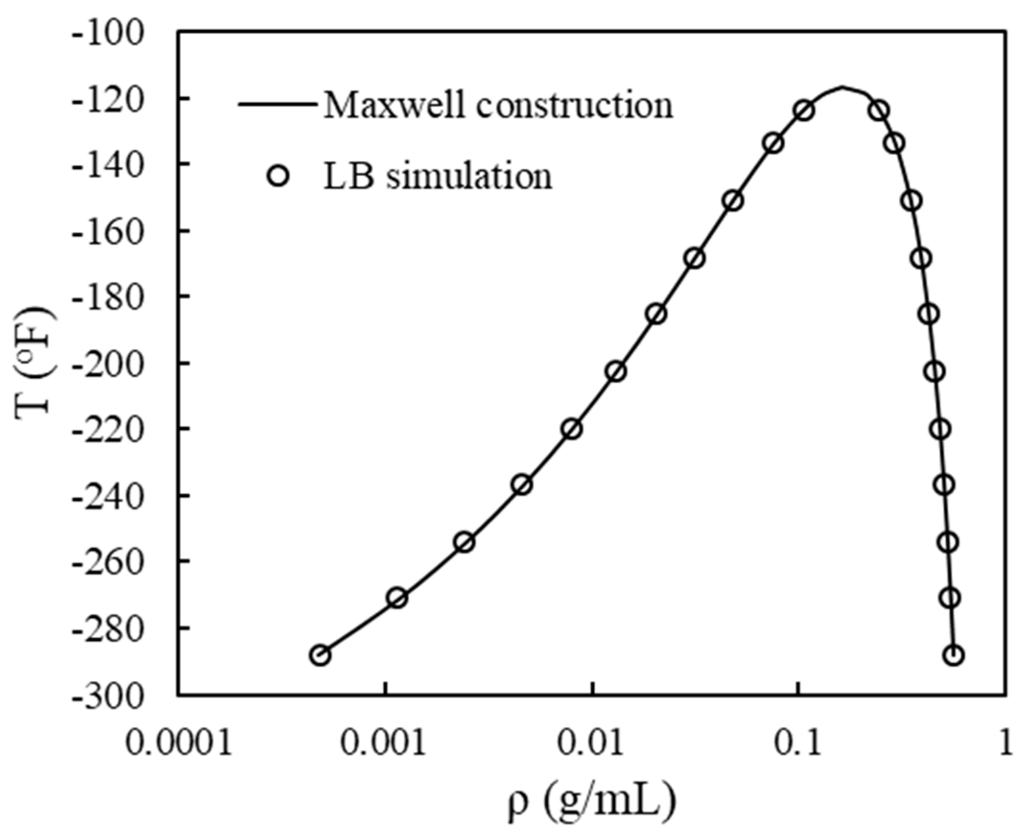
In this part, we first evaluate the phase separation of methane at the bulk condition. Simulation is conducted in a 1003 domain. The periodic boundary condition is applied at x, y, z-direction so that methane can be regarded as bulk gas. Initially, the computational domain is filled with methane with equal density everywhere and the temperature is set below the critical temperature. By a small perturbation applied, phase separation of methane can be achieved due to the intermolecular interactions. In this way, liquid and vapor densities of methane at the temperature are obtained from simulation. Repeating the same process in different temperatures, we can construct the coexistence curve using the LB method. In Figure 1, the coexistence curve from the simulation is compared with the theoretical one obtained using Maxwell construction on PR-EOS. The good match indicates the reliability of this method for phase behavior study.
After simulating phase equilibrium at bulk condition, phase change in a slit pore is studied. The simulation setup is shown in Figure 2. A three-dimensional capillary tube with a rectangular cross-section is used. The solid boundary condition is applied in the y and z-direction. In x-direction, constant pressure is held at the entrances of the tube. Similar to the case of bulk gas, the tube is initially filled with methane with equal density everywhere and the temperature is below the critical temperature. At inlet and outlet boundaries, the pressure/density of the gas is fixed. By gradually increasing the density of gas at the boundary, the change of average density inside the tube is recorded. Figure 3 presents examples of average densities as functions of densities at the boundary at three temperatures. The length of the side of the tube is 10 nm. Clearly, the average density undergoes a sudden jump, from a vapor-like density to liquid-like density. This sudden change of average density inside the tube indicates the occurrence of capillary condensation. The average densities right before and immediately after the sudden jump are regarded as the vapor and liquid densities at a specific temperature. By following the same procedure using different temperatures, we can construct the coexistence curve in the capillary tube.
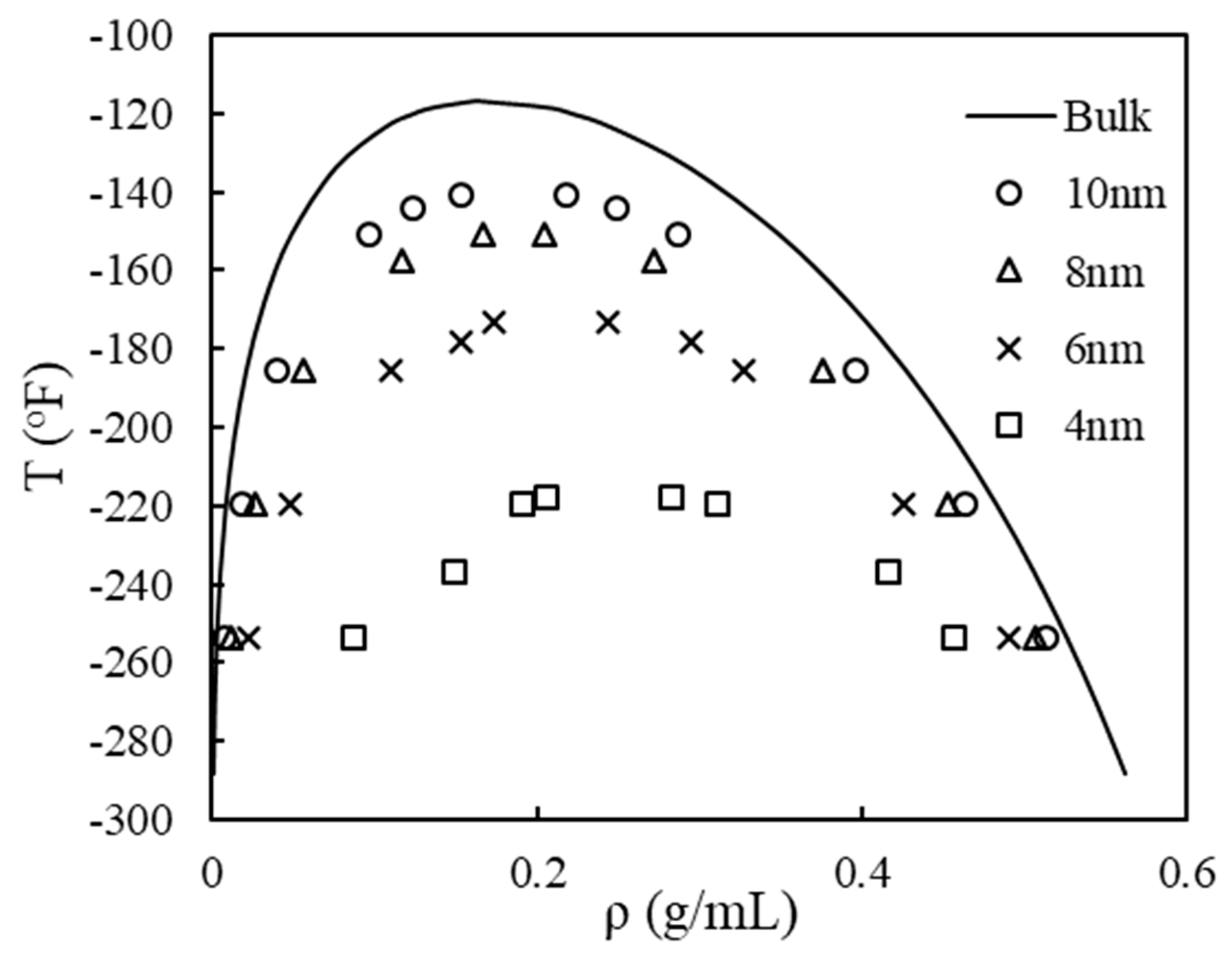
In Figure 4, the coexistence curves of methane in different sizes of nanotubes are compared with that at the bulk condition. The liquid-gas contact angle is assumed to be 30°. A significant shift of the coexistence curve is observed in the nanotube, especially when the size of the tube is small. Compared to bulk condition, liquid density is decreased and vapor density is increased. Also, a clear shift of critical point is observed in nanopores. Specifically, the critical temperature decreases, and critical density increases with decreasing pore sizes. The shifted critical properties are consistent with results using molecular simulation [21,22] and density function theory [26,27].
3.2. Phase Equilibrium with the Pore Size Distribution
In Section 3.1, we have shown the calculation of phase equilibrium in a single capillary tube. However, it is known that pore size in shale always yields a distribution [4]. Thus, it is important to study phase behavior in a medium with distributed pore sizes. As shown in Figure 5, normalized pore size data of a shale sample from Eagle Ford is used [49]. The measured data is from Hg intrusion [49]. Four representative pore sizes are used to represent the distributed pores. Note that the choice is not unique. The chosen representative pore size should have relatively high pore volume and significantly deviated phase behavior. As illustrated in Figure 5, pore sizes of 4 nm, 6 nm, 8 nm, and 14 nm are chosen to cover the pores with sizes of 3–5 nm, 5–7 nm, 7–9 nm, 9–30 nm respectively. The pore volume of each size of pores equals the volume of pores covered. Following the work of Jin et al. [50], pores larger than 30 nm are ignored where the confinement effect on phase behavior can be ignored.
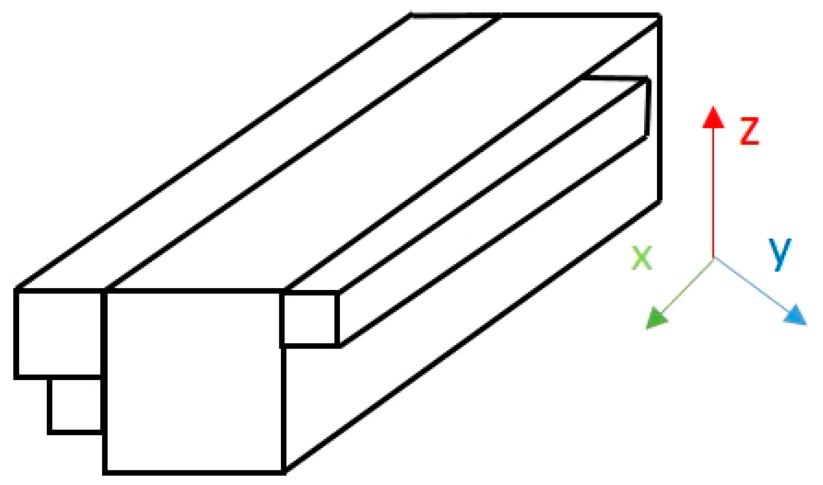
To study the effect of pore size distribution on phase behavior using LB, a bundle of capillary tubes is used. The simuation setup is shown in Figure 6. Four capillary tubes are arranged in parallel with the side length of 4 nm, 6 nm, 8 nm, and 14 nm respectively. The length of tubes in x-direction is determined by the volume fraction occupied by each pore. Similar to the study in a single capillary tube, the solid boundary condition is applied in the y and z direction and the pressure boundary condition is applied in the x-direction. Then, the tubes are filled by increasing the gas density at the boundary. Since the tubes have different sizes and volumes, the volume of the bundle is the summation of the volume of each tube. We consider the average density of the bundle over the whole volume. With different sizes of tubes, condensation may happen first in small tubes. Due to the shared boundary, fluids in small tubes may exchange mass with fluids in other tubes.
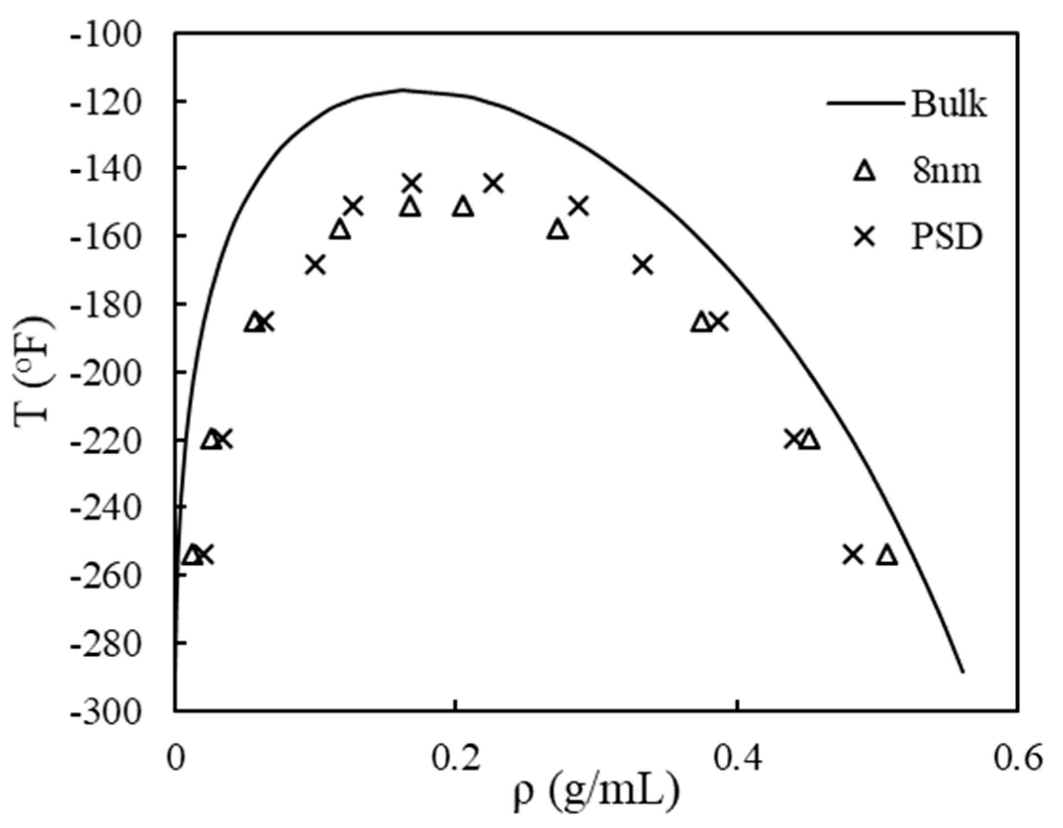
Following the procedure in Section 3.1, the coexistence curve of methane in the bundle of capillary tubes can be established which is shown in Figure 7. Since it is not straightforward to directly apply pore size distribution into modified EOS or reservoir simulation, we choose to use one pore size to represent the effect of pore size distribution on confined phase behavior. As illustrated in Figure 7, the coexistence in the capillary bundle is close to the one in the 8 nm capillary tube. Thus, we consider 8 nm as the ‘effective’ pore size for this rock when calculating confined phase behavior.
3.3. Modified EOS from Pore-Scale Simulation
With shifted coexistence curve, a modified EOS can be built to account for the effects of confinement. Different forms of EOS have been proposed in the literature [35,36,37]. In this work, a modified EOS in Equation (23) is used to match with the simulation data [2].
The modified and account for the changed impulsive and repulsive forces in confined space. By carefully tuning the value of the above parameters, the coexistence curve from the modified EOS can match with simulation data. As shown in Figure 8, the modified EOS can capture the shift of the coexistence curve correctly. Compared to results from LB simulation, vapor densities from modified EOS have a good match with simulation. Liquid density is well predicted at high temperatures but overestimated at low temperatures. Note that the EOS used for matching the simulation data is not unique. Readers can use any form of EOS and a better match could be obtained.
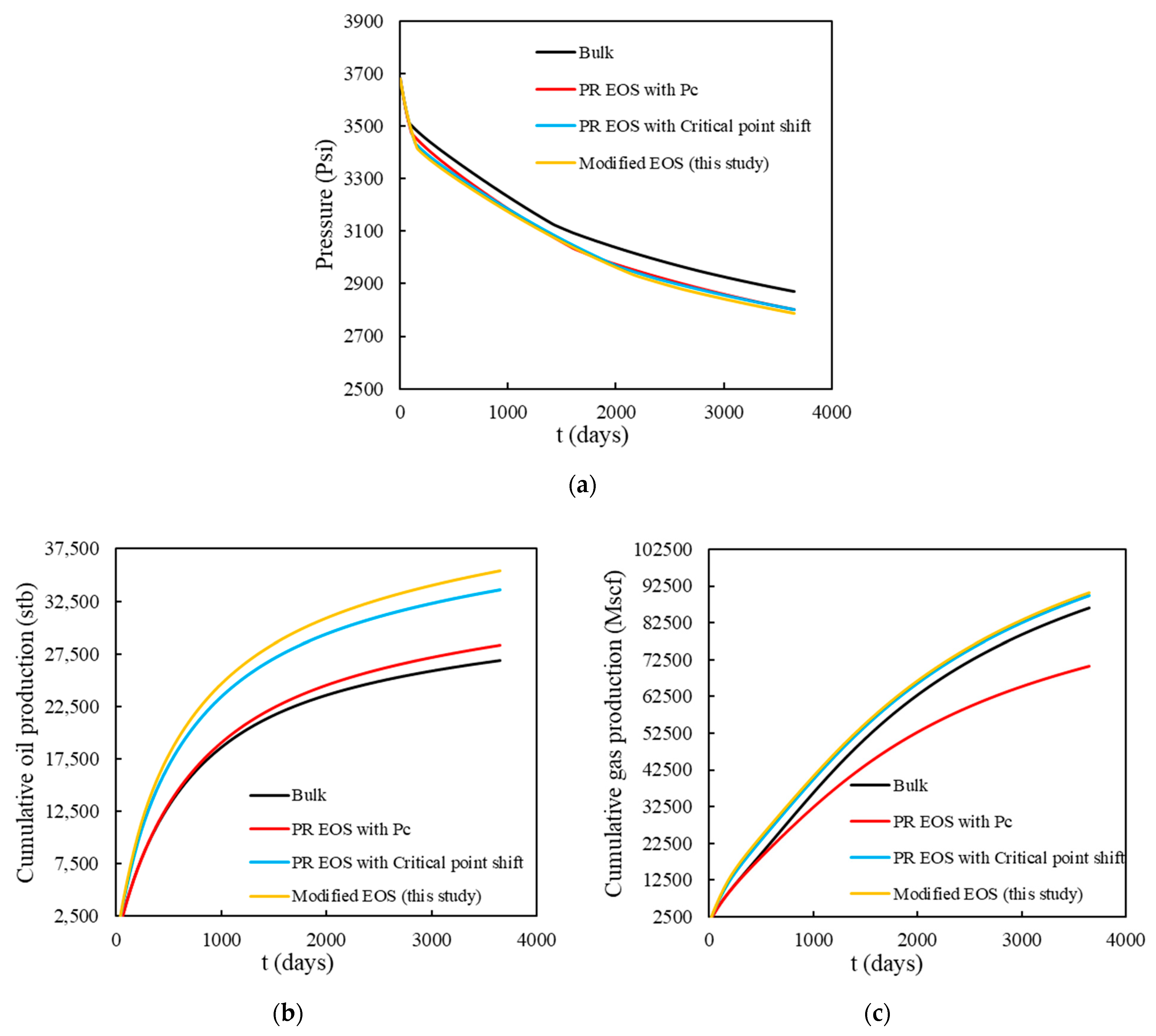
The modified EOS is then extended to model the confined phase behavior of shale oil. The fluid model used is shown in Table 1 and Table 2. The P–T phase diagram of shale oil using the modified EOS is presented in Figure 9. The pore diameter used for thermodynamic modeling is 8 nm. In the literature, implementing capillary pressure and critical shift method are the two commonly used methods for confined phase behavior. To make a comparison, we also plot the phase diagrams using the two methods as well as that at the bulk condition in Figure 9. Compared to bulk, all three methods generate shifted phase diagrams, and suppressed bubble point pressures are observed. However, the method of implementing capillary pressure cannot capture the changed critical point. The modified EOS in this study and critical shift method using Equations (18) and (19) can both capture the shift of critical point. Qualitatively, the shift is more significant when using the modified EOS. In Figure 10, the saturation pressures in different sizes of pores are compared when T = 240 °F. It is seen that saturation pressures decrease linearly with the increasing inverse of pore size. Also, the suppression of saturation pressure is more significant in all sizes of pores when using the modified EOS.
3.4. Compositional Simulation of Shale Reservoir Considering Confined Phase Bahavior
As illustrated in Section 3.3, the shifted phase diagram and saturation pressure of shale oil indicate that the properties of oil and gas should also be altered in nanopores, which in turn will affect the predicted oil and gas production. To evaluate the production of shale oil reservoirs using the different EOS, the fractured shale reservoir shown in Figure 11 is studied. As shown, a horizontal well is drilled in the middle of the 2D reservoir (shown as a bold black line). The red lines represent 17 stages of hydraulic fractures that are connected with the well. The properties of shale matrix and hydraulic fractures are summarized in Table 3. This small reservoir should be regarded as the SRV (stimulated reservoir volume). Apply no-flow boundary to the outer bound of this reservoir and production is constrained by constant bottom-hole pressure. As illustrated in Figure 8, we use 8 nm as the effective pore size for the shale matrix. The bubble point pressure of this oil sample in 8 nm pore is 2630 psi, 2345 psi, and 2105 psi when using methods of capillary pressure, critical shift, and modified EOS respectively. At bulk condition, the bubble point pressure is 2768 psi. At initial reservoir pressure (3700 psi), the fluid shale matrix is thus pure oil. At a later stage of production, gas starts to appear and three-phase flow will be involved. The three-phase relative permeability in Figure 12 is applied for flow in the shale matrix. In the fractures, assume that the relative permeabilities are a linear function with saturations.
Simulated production from the REV using different confined models are presented in Figure 13 including reservoir pressure, cumulative oil production, and cumulative gas production. As shown in Figure 13a, compared to bulk condition, implementing confined phase behavior leads to a faster pressure decline. In terms of the rate of pressure decline, there is not much difference between the methods of capillary pressure, critical shift, and modified EOS used in this study. However, the oil and gas production is quite different when using different methods. As illustrated in Figure 13b, the cumulative oil production is higher if confined phase behavior is considered. The use of modified EOS in this study leads to the highest oil production. Oil production considering critical shift is second high followed by that using capillary pressure. The increased oil production rate is due to the suppressed bubble point in nanopores. It is apparent that more oil production can be expected if the suppression of bubble point is more significant. On the other hand, gas production is lower than that at bulk condition if only capillary pressure is considered. However, gas production is higher if the shift of critical points or modified EOS in this study is applied. Cumulative gas productions are close between the methods of critical shift and modified EOS. The comparison of cumulative gas productions using different method are presented in Figure 13c.
Since we only studied a simplified reservoir model in this work, a direct comparison with field data is not possible. The aim of this work is to provide an insight for simulation of shale reservoir in terms of altered phase behavior. As discussed above, the effects of different methods of confined phase behavior on oil/gas production from shale reservoirs cannot be ignored. The method of implementing capillary pressure fails to capture the altered critical points in nanopores. Considering capillary pressure alone is not sufficient to model confined phase behavior and both oil and gas production will be underestimated. Applying the critical shift method from Zarragoicoechea and Kuz [32] and modified EOS leads to higher oil and gas production. Besides, it is observed that the modified EOS has close performance with the critical shift method in predicting gas production but different in predicting oil production. The difference between these two methods requires more work in the future including comparison with experimental results or other methods.
4. Conclusions
In this work, we conducted a pore-scale simulation of confined phase behavior using the pseudo-potential LB method. The model was validated with Peng-Robinson equation of state at bulk condition. Vapor-liquid equilibrium in nanopores was simulated by modelling adsorption isotherms in capillary tubes. A sudden jump in adsorption isotherms indicated the occurrence of capillary condensation in nanopores. In addition, effect of pore size distribution on phase equilibrium is evaluated by using a bundle of capillary tubes with varied sizes. Size and volume fraction of each tube is determined by matching with experimental data of pore size. To include the deviated phase equilibrium into a reservoir-scale simulation, a modified EOS is built guided by results from LB simulation. The following conclusions can be made in this study:
- By comparing constructed coexistence curves, we propose that an effective pore size can be used to represent a real rock sample with distributed nanopores.
- Shifted critical properties and suppressed bubble points were observed when using the modified EOS.
- Compared to methods using capillary pressure and critical shift, the phase diagram using modified EOS shrinks more significantly.
- Compositional simulation indicated that both oil and gas production will increase if modified EOS is implemented. Considering capillary pressure or shifted critical point only will underestimate oil and gas production and ultimate recovery from shale reservoir.
Author Contributions
Conceptualization, J.H.; methodology, J.H.; formal analysis, J.H. and H.W.; writing—original draft preparation, J.H.; writing—review and editing, H.W. All authors have read and agreed to the published version of the manuscript.
Funding
No funding is reported for this work.
Data Availability Statement
Not applicable.
Conflicts of Interest
The authors declare no conflicts of interest.
Nomenclature
| discrete set of velocity vectors | |
| fugacity of component i in liquid phase | |
| fugacity of component i in vapor phase | |
| velocity distribution function of particles | |
| distribution function at equilibrium state | |
| fluid pressure, Psi | |
| critical pressure, Psi | |
| capillary pressure, Psi | |
| pore radius, nm | |
| universal gas constant | |
| switch function, 0 or 1 | |
| oil saturation | |
| gas saturation | |
| critical temperature, °F | |
| initial width of interface | |
| position of particles | |
| fluid density, g/mL | |
| liquid density, g/mL | |
| vapor density, g/mL | |
| fluid viscosity | |
| pseudopotential | |
| weighting parameter | |
| interfacial tension in real unit [N/m] | |
| contact angle | |
| porosity |
References
- Yu, W.; Lashgari, H.R.; Wu, K.; Sepehrnoori, K. CO2 injection for enhanced oil recovery in Bakken tight oil reservoirs. Fuel 2015, 159, 354–363. [Google Scholar] [CrossRef]
- Hu, X.; Li, M.; Peng, C.; Davarpanah, A. Hybrid thermal-chemical enhanced oil recovery methods; an experimental study for tight reservoirs. Symmetry 2020, 12, 947. [Google Scholar] [CrossRef]
- Hu, X.; Xie, J.; Cai, W.; Wang, R.; Davarpanah, A. Thermodynamic effects of cycling carbon dioxide injectivity in shale reservoirs. J. Pet. Sci. Eng. 2020, V195, 107717. [Google Scholar] [CrossRef]
- Yang, G.; Fan, Z.; Li, X. Determination of confined fluid phase behavior using extended Peng-Robinson equation of state. Chem. Eng. J. 2019, 378, 122032. [Google Scholar] [CrossRef]
- Pommer, M.; Milliken, K. Pore types and pore-size distributions across thermal maturity, Eagle Ford Formation, southern Texas. AAPG Bull. 2015, 99, 1713–1744. [Google Scholar] [CrossRef]
- Nojabaei, B.; Johns, R.T.; Chu, L. Effect of capillary pressure on phase behavior in tight rocks and shales. SPE Reserv. Eval. Eng. 2013, 16, 281–289. [Google Scholar] [CrossRef]
- Davarpanah, A.; Mirshekari, B. Experimental Investigation and Mathematical Modeling of Gas Diffusivity by Carbon Dioxide and Methane Kinetic Adsorption. Ind. Eng. Chem. Res. 2019, 58, 12392–12400. [Google Scholar] [CrossRef]
- Sanaei, A.; Ma, Y.; Jamili, A. Nanopore Confinement and Pore Connectivity Considerations in Modeling Unconventional Resources. J. Energy Resour. Technol. 2019, 141, 012904. [Google Scholar] [CrossRef]
- Qiao, S.Z.; Bhatia, S.K.; Nicholson, D. Study of hexane adsorption in nanoporous MCM-41 silica. Langmuir 2004, 20, 389–395. [Google Scholar] [CrossRef]
- Russo, P.A.; Carrott, M.M.L.R.; Carrott, P.J.M. Hydrocarbons adsorption on templated mesoporous materials: Effect of the pore size, geometry and surface chemistry. New J. Chem. 2011, 35, 407–416. [Google Scholar] [CrossRef]
- Morishige, K.; Fujii, H.; Uga, M.; Kinukawa, D. Capillary critical point of argon, nitrogen, oxygen, ethylene, and carbon dioxide in MCM-41. Langmuir 1997, 13, 3494–3498. [Google Scholar] [CrossRef]
- Wang, L.; Parsa, E.; Gao, Y.; Ok, J.T.; Neeves, K.; Yin, X.; Ozkan, E. Experimental study and modeling of the effect of nanoconfinement on hydrocarbon phase behavior in unconventional reservoirs. In Proceedings of the SPE Western North American and Rocky Mountain Joint Meeting, Denver, CO, USA, 17–18 April 2014. [Google Scholar]
- Parsa, E.; Yin, X.; Ozkan, E. Direct observation of the impact of nanopore confinement on petroleum gas condensation. In Proceedings of the SPE Annual Technical Conference and Exhibition, Society of Petroleum Engineers, Houston, TX, USA, 27–30 September 2015. [Google Scholar]
- Alfi, M.; Nasrabadi, H.; Banerjee, D. Experimental investigation of confinement effect on phase behavior of hexane, heptane and octane using lab-on-a-chip technology. Fluid Phase Equilib. 2016, 423, 25–33. [Google Scholar] [CrossRef]
- Alfi, M.; Nasrabadi, H.; Banerjee, D. Effect of confinement on bubble point temperature shift of hydrocarbon mixtures: Experimental investigation using nanofluidic devices. In Proceedings of the SPE Annual Technical Conference and Exhibition, San Antonio, TX, USA, 9–11 October 2017. [Google Scholar]
- Yang, Q.; Jin, B.; Banerjee, D.; Nasrabadi, H. Direct visualization and molecular simulation of dew point pressure of a confined fluid in sub-10nm slit pores. Fuel 2019, 235, 1216–1223. [Google Scholar] [CrossRef]
- Sedghi, M.; Piri, M. Capillary condensation and capillary pressure of methane in carbon nanopores: Molecular Dynamics simulations of nanoconfinement effects. Fluid Phase Equilib. 2018, 459, 196–207. [Google Scholar] [CrossRef]
- Ambrose, R.J.; Hartman, R.C.; Diaz-Campos, M.; Akkutlu, I.Y.; Sondergeld, C.H. Shale gas-in-place calculations part I: New pore-scale considerations. SPE J. 2012, 17, 219–229. [Google Scholar] [CrossRef]
- Peterson, B.K.; Gubbins, K.E. Phase transitions in a cylindrical pore. Mol. Phys. 1987, 62, 215–226. [Google Scholar] [CrossRef]
- Hamada, Y.; Koga, K.; Tanaka, H. Phase equilibria and interfacial tension of fluids confined in narrow pores. J. Chem. Phys. 2007, 127, 084908. [Google Scholar] [CrossRef] [PubMed] [Green Version]
- Singh, S.K.; Sinha, A.; Deo, G.; Singh, J.K. Vapor−liquid phase coexistence, critical properties, and surface tension of confined alkanes. J. Phys. Chem. C 2009, 113, 7170–7180. [Google Scholar] [CrossRef]
- Singh, S.K.; Singh, J.K. Effect of pore morphology on vapor–liquid phase transition and crossover behavior of critical properties from 3D to 2D. Fluid Phase Equilib. 2011, 300, 182–187. [Google Scholar] [CrossRef]
- Vishnyakov, A.; Piotrovskaya, E.M.; Brodskaya, E.N.; Tovbin, Y.K. Critical properties of Lennard-Jones fluids in narrow slit-shaped pores. Langmuir 2001, 17, 4451–4458. [Google Scholar] [CrossRef]
- Huang, J.; Yin, X.; Killough, J. Thermodynamic consistency of a pseudopotential lattice Boltzmann fluid with interface curvature. Phys. Rev. E 2019, 100, 053304. [Google Scholar] [CrossRef]
- Huang, J.; Yin, X.; Barrufet, M.; Killough, J. Lattice Boltzmann Simulation of Phase Behavior of Hydrocarbons in Nanopores: Role of Capillary Pressure and Fluid-Solid Interaction. In Proceedings of the SPE Annual Technical Conference and Exhibition, Denver, CO, USA, 26–29 October 2020. SPE-201458-MS. [Google Scholar]
- Li, Z.; Firoozabadi, A. Interfacial tension of nonassociating pure substances and binary mixtures by density functional theory combined with Peng–Robinson equation of state. J. Chem. Phys. 2009, 130, 154108. [Google Scholar] [CrossRef]
- Jin, Z.; Firoozabadi, A. Thermodynamic Modeling of Phase Behavior in Shale Media. SPE J. 2016, 21, 190–207. [Google Scholar] [CrossRef] [Green Version]
- Li, Z.; Jin, Z.; Firoozabadi, A. Phase behavior and adsorption of pure substances and mixtures and characterization in nanopore structures by density functional theory. SPE J. 2014, 19, 1096–1109. [Google Scholar] [CrossRef] [Green Version]
- Stimpson, B.C.; Barrufet, M.A. Thermodynamic Modeling of Pure Components Including the Effects of Capillarity. J. Chem. Eng. Data 2016, 61, 2844–2850. [Google Scholar] [CrossRef]
- Du, F.; Nojabaei, B. A black-oil approach to model produced gas injection in both conventional and tight oil-rich reservoirs to enhance oil recovery. Fuel 2020, V263, 116680. [Google Scholar] [CrossRef]
- Huang, J.; Jin, T.; Chai, Z.; Barrufet, M.; Killough, J. Compositional simulation of fractured shale reservoir with distribution of nanopores using coupled multi-porosity and EDFM method. J. Pet. Sci. Eng. 2019, 179, 1078–1089. [Google Scholar] [CrossRef]
- Zarragoicoechea, G.J.; Kuz, V.A. Critical shift of a confined fluid in a nanopore. Fluid Phase Equilib. 2004, 220, 7–9. [Google Scholar] [CrossRef]
- Alharthy, N.S.; Nguyen, T.; Teklu, T.; Kazemi, H.; Graves, R. Multiphase compositional modeling in small-scale pores of unconventional shale reservoirs. In Proceedings of the SPE Annual Technical Conference and Exhibition, Society of Petroleum Engineers, New Orleans, LA, USA, 30 September–2 October 2013. [Google Scholar]
- Du, F.; Huang, J.; Chai, Z.; Killough, J. Effect of vertical heterogeneity and nano-confinement on the recovery performance of oil-rich shale reservoir. Fuel 2020, 267, 117199. [Google Scholar] [CrossRef]
- Luo, S.; Jin, B.; Lutkenhaus, J.L.; Nasrabadi, H. A novel pore-size-dependent equation of state for modeling fluid phase behavior in nanopores. Fluid Phase Equilib. 2019, 498, 72–85. [Google Scholar] [CrossRef]
- Travalloni, L.; Castier, M.; Tavares, F.W. Phase equilibrium of fluids confined in porous media from an extended Peng-Robinson equation of state, Fluid Phase Equilib. 2014, 362, 335–341. Fluid Phase Equilib. 2014, 362, 335–341. [Google Scholar] [CrossRef]
- Wang, Y.; Aryana, S.A. Coupled confined phase behavior and transport of methane in slit nanopores. Chem. Eng. J. 2021, 404, 126502. [Google Scholar] [CrossRef]
- Zhang, Y.; Yu, W.; Sepehrnoori, K.; Di, Y. Investigation of nanopore confinement on fluid flow in tight reservoirs. J. Petrol. Sci. Eng. 2017, 150, 265–271. [Google Scholar] [CrossRef]
- Haider, B.A.; Aziz, K. Impact of Capillary Pressure and Critical Property Shift due to Confinement on Hydrocarbon Production in Shale Reservoirs. In Proceedings of the SPE Reservoir Simulation Conference, Montgomery, TX, USA, 20–22 February 2017. Paper Number: SPE-182603-MS. [Google Scholar]
- Song, Z.; Song, Y.; Guo, J.; Feng, D.; Dong, J. Effect of Nanopore Confinement on Fluid Phase Behavior and Production Performance in Shale Oil Reservoir. Ind. Eng. Chem. Res. 2021, 60, 1463–1472. [Google Scholar] [CrossRef]
- d’Humières, D. Multiple–relaxation–time lattice Boltzmann models in three dimensions. Philosophical Transactions of the Royal Society of London. Ser. A Math. Phys. Eng. Sci. 2002, 360, 437–451. [Google Scholar]
- Gong, S.; Cheng, P. Numerical investigation of droplet motion and coalescence by an improved lattice Boltzmann model for phase transitions and multiphase flows, Comput. Fluids 2012, 53, 93–104. [Google Scholar]
- Yuan, P.; Schaefer, L. Equations of state in a lattice Boltzmann model. Phys. Fluids 2006, 18, 042101. [Google Scholar] [CrossRef]
- Li, Q.; Luo, K.H.; Kang, Q.J.; Chen, Q. Contact angles in the pseudopotential lattice Boltzmann modeling of wetting. Phys. Rev. E. 2014, 2014, 053301. [Google Scholar] [CrossRef] [Green Version]
- Kupershtokh, A.L.; Medvedev, D.A.; Karpov, D.I. On equations of state in a lattice Boltzmann method. Comput. Math. Appl. 2009, 58, 965–974. [Google Scholar] [CrossRef] [Green Version]
- Yan, B.; Wang, Y.; Killough, J.E. A fully compositional model considering the effect of nanopores in tight oil reservoirs. J. Pet. Sci. Eng. 2017, 152, 675–682. [Google Scholar] [CrossRef]
- Chai, Z.; Yan, B.; Killough, J.E.; Wang, Y. An efficient method for fractured shale reservoir history matching: The embedded discrete fracture multi-continuum approach. J. Pet. Sci. Eng. 2018, 160, 170–181. [Google Scholar] [CrossRef]
- Chai, Z.; Tang, H.; He, Y.; Killough, J.E.; Wang, Y. Uncertainty Quantification of the Fracture Network with a Novel Fractured Reservoir Forward Model. In Proceedings of the SPE Annual Technical Conference and Exhibition, Dallas, TX, USA, 24–26 September 2018. SPE-191395-MS. [Google Scholar]
- Clarkson, C.R.; Solano, N.; Bustin, R.M.; Bustin, A.M.M.; Chalmers, G.R.L.; He, L.; Melnichenko, Y.B.; RadliÅski, A.P.; Blach, T.P. Pore structure characterization of north american shale gas reservoirs using usans/sans, gas adsorption, and mercury intrusion. Fuel 2013, 103, 606–616. [Google Scholar] [CrossRef]
- Jin, B.; Bi, R.; Nasrabadi, H. Molecular simulation of the pore size distribution effect on phase behavior of methane confined in nanopores. Fluid Phase Equilib. 2017, V452, 94–102. [Google Scholar] [CrossRef]
Figure 1.
Coexistence curves of methane from LB simulation and Maxwell construction on PR-EOS.

Figure 2.
Simulation setup for phase equilibrium in a single capillary tube.
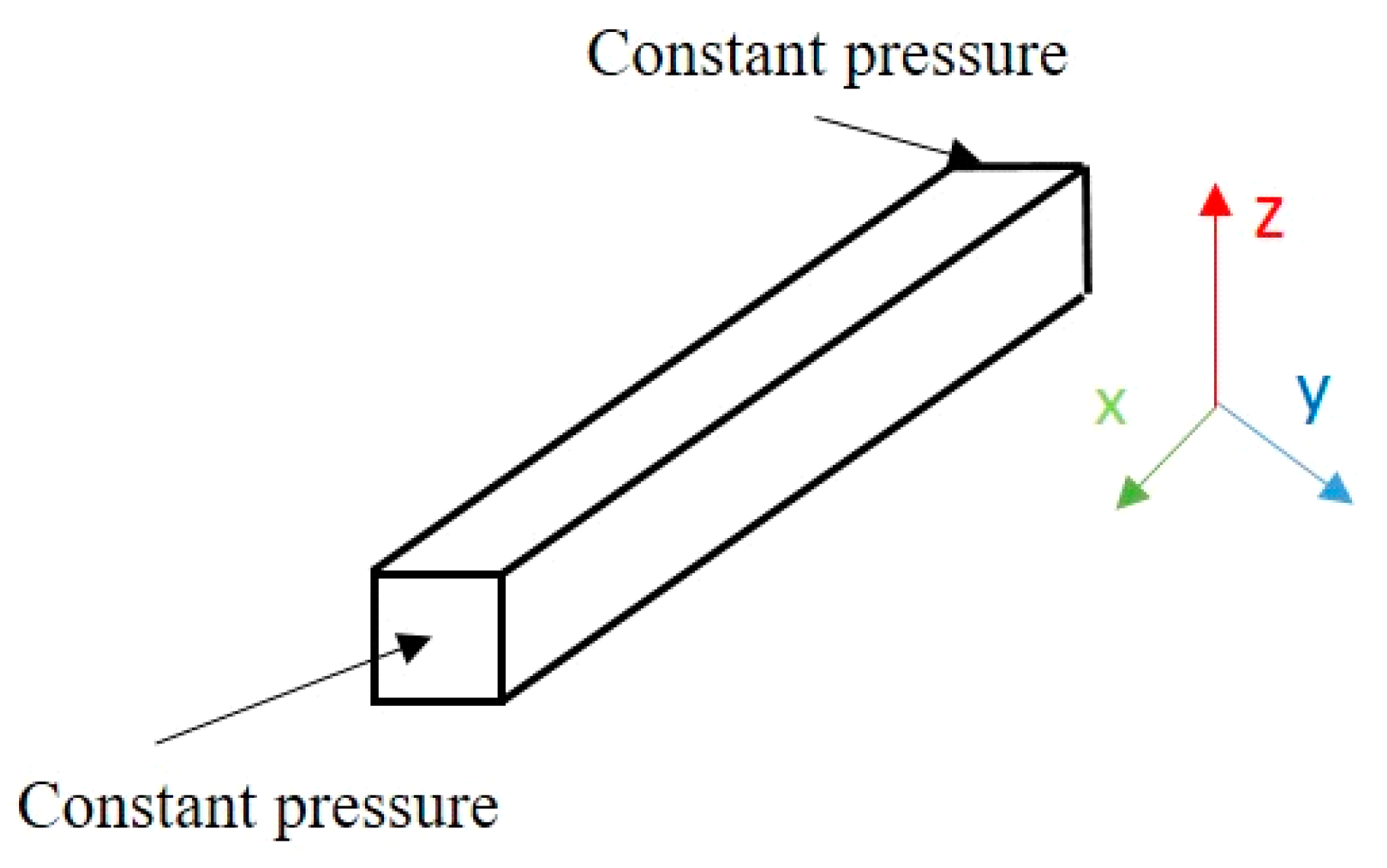
Figure 3.
Average density in a 10 nm capillary tube changes with density at boundary under different temperatures.
Figure 3.
Average density in a 10 nm capillary tube changes with density at boundary under different temperatures.

Figure 4.
Simulated coexistence curves of methane in different sizes of capillary tubes uing LB method.
Figure 4.
Simulated coexistence curves of methane in different sizes of capillary tubes uing LB method.

Figure 5.
Normalized pore size distribution of shale rock obtained from experiments (data obtained from [50]) and discrete pore size distribution used in LB simulation. PSD represents pore size distribution.
Figure 5.
Normalized pore size distribution of shale rock obtained from experiments (data obtained from [50]) and discrete pore size distribution used in LB simulation. PSD represents pore size distribution.
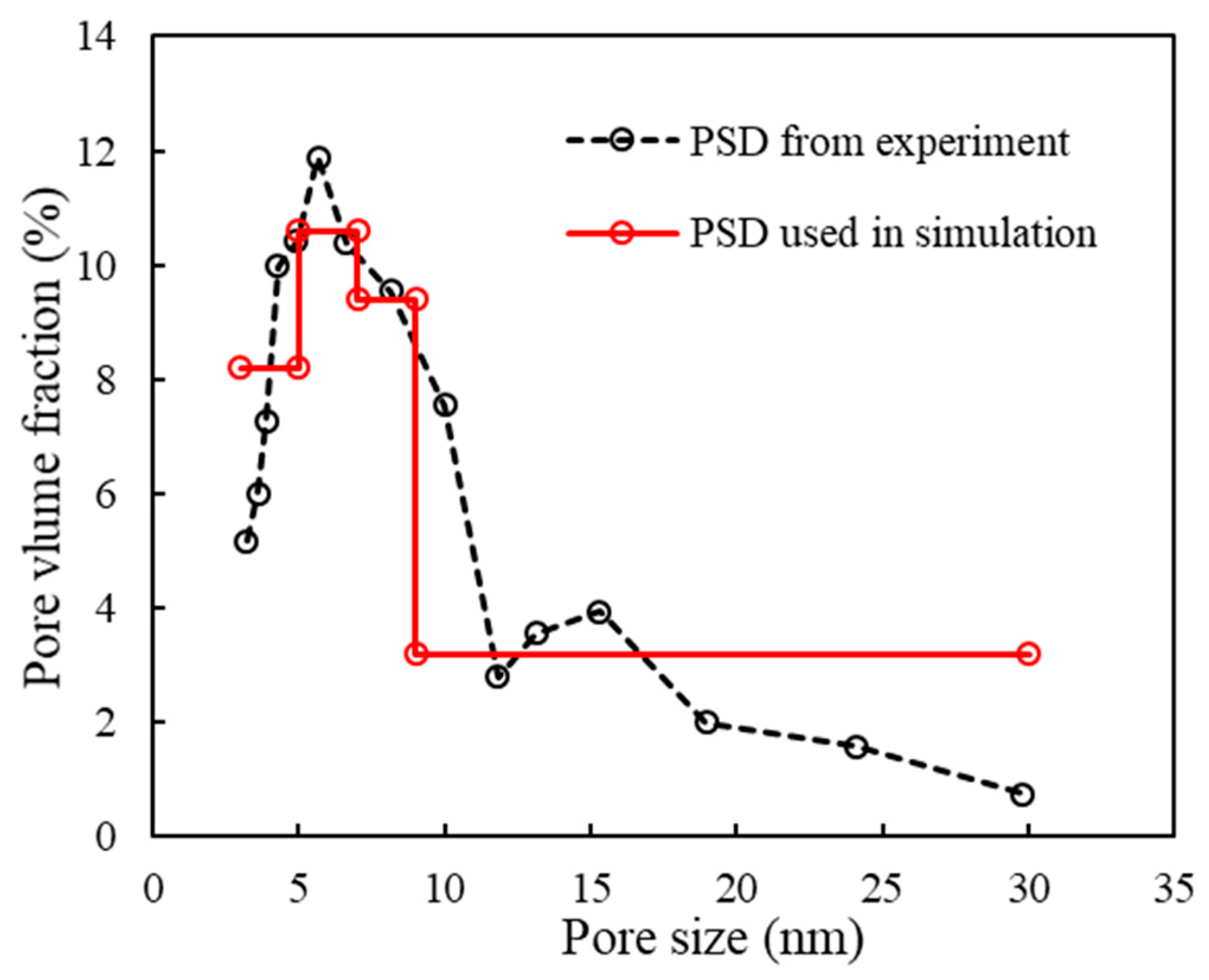
Figure 6.
A bundle of capillary tubes used for studying confined phase behavior with pore size distribution.
Figure 6.
A bundle of capillary tubes used for studying confined phase behavior with pore size distribution.

Figure 7.
Simulated coexistence curves of methane with pore size distribution and in an 8 nm single capillary tube. PSD represents pore size distribution.
Figure 7.
Simulated coexistence curves of methane with pore size distribution and in an 8 nm single capillary tube. PSD represents pore size distribution.

Figure 8.
Comparison of coexistence curves of methane using PR EOS, modified EOS, and LB simulation.
Figure 8.
Comparison of coexistence curves of methane using PR EOS, modified EOS, and LB simulation.

Figure 9.
Comparison of P-T phase diagrams of shale oil at the bulk condition with those using methods of capillary pressure, critical shift, and modified EOS in this study. Black points represent critical points.
Figure 9.
Comparison of P-T phase diagrams of shale oil at the bulk condition with those using methods of capillary pressure, critical shift, and modified EOS in this study. Black points represent critical points.

Figure 10.
Calculated saturation pressures in different size of nanopores when using methods of capillary pressure, critical shift, and modified EOS at T = 240 °F.
Figure 10.
Calculated saturation pressures in different size of nanopores when using methods of capillary pressure, critical shift, and modified EOS at T = 240 °F.
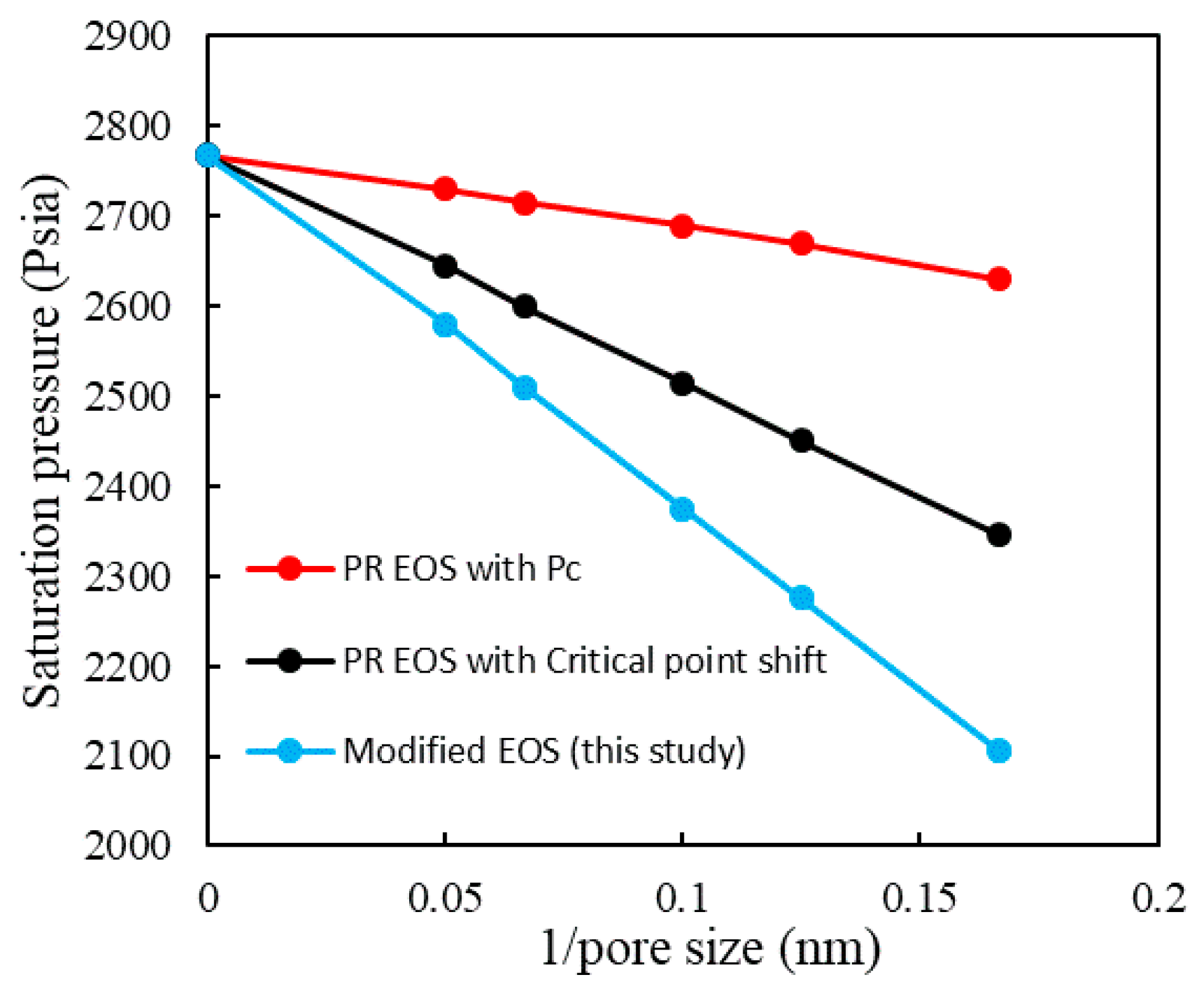
Figure 11.
Simulated REV of shale reservoir used in simulation; bold black line in the middle is the horizontal well and red lines represent 17 stages of hydraulic fractures.
Figure 11.
Simulated REV of shale reservoir used in simulation; bold black line in the middle is the horizontal well and red lines represent 17 stages of hydraulic fractures.
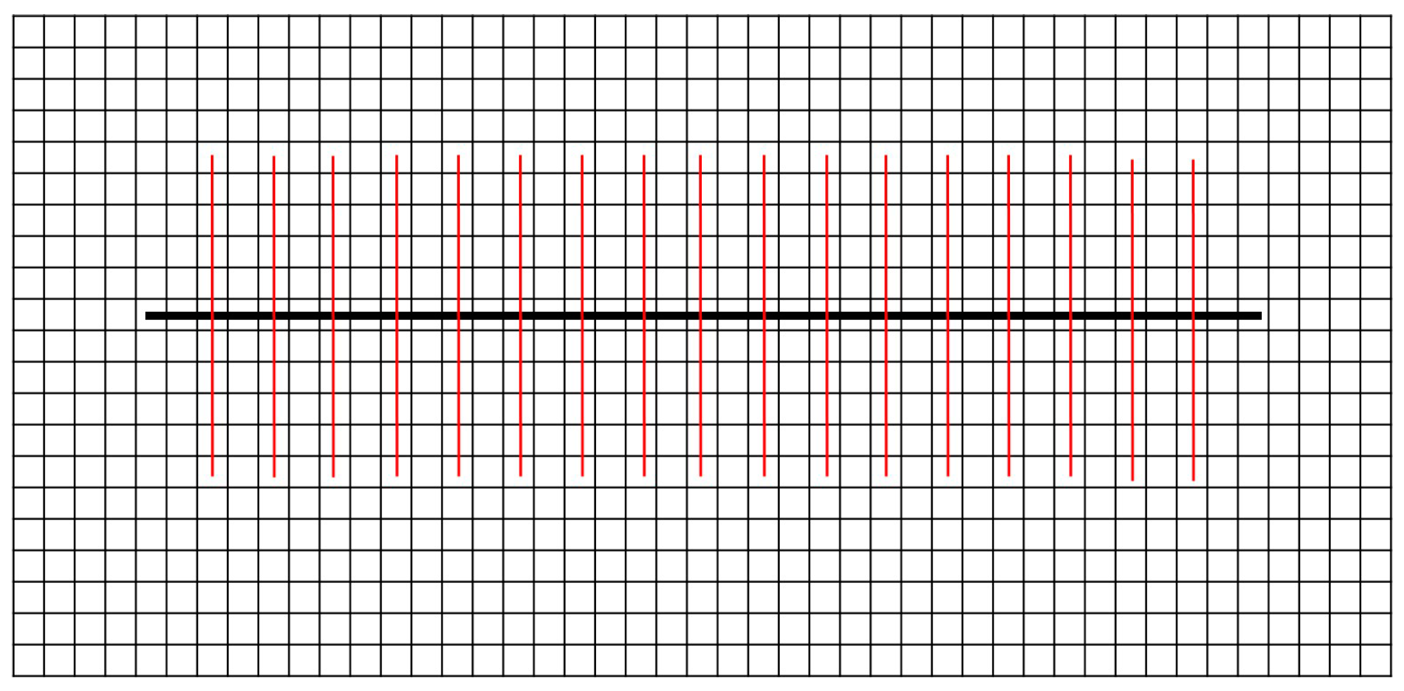
Figure 12.
Oil-water relative permeability (a) and oil-gas relative permeability (b) in shale matrix.
Figure 12.
Oil-water relative permeability (a) and oil-gas relative permeability (b) in shale matrix.

Figure 13.
Comparison of reservoir performance from compositional simulation using methods of capillary pressure, critical shift, and modified EOS; (a) reservoir pressure, (b) cumulative oil production, and (c) cumulative gas production.
Figure 13.
Comparison of reservoir performance from compositional simulation using methods of capillary pressure, critical shift, and modified EOS; (a) reservoir pressure, (b) cumulative oil production, and (c) cumulative gas production.

Table 1.
Mole fraction and basic properties of studied fluid [34].
Table 1.
Mole fraction and basic properties of studied fluid [34].
| Component | Mole Fraction | Critical Pressure (Psia) | Critical Temperature (°F) | Acentric Factor | Mole Weight | Parachor |
|---|---|---|---|---|---|---|
| C1 | 0.36736 | 655.02 | −124.33 | 0.01020 | 16.54 | 74.8 |
| C2–C3 | 0.24219 | 681.05 | 135.01 | 0.12176 | 35.70 | 124.7 |
| C4–C6 | 0.12157 | 501.58 | 360.81 | 0.23103 | 68.75 | 221.5 |
| C7–C12 | 0.15854 | 363.34 | 593.58 | 0.42910 | 120.56 | 350.2 |
| C13–C80 | 0.11034 | 229.64 | 1044.43 | 0.81953 | 295.51 | 800.4 |
Table 2.
Binary interaction coefficient of studied fluid [34].
Table 2.
Binary interaction coefficient of studied fluid [34].
| C1 | C2–C3 | C4–C6 | C7–C12 | C13–C80 | |
|---|---|---|---|---|---|
| C1 | 0 | ||||
| C2–C3 | 0.0044 | 0 | |||
| C4–C6 | 0.0036 | 0.0019 | 0 | ||
| C7–C12 | 0.0033 | 0.0016 | 0 | 0 | |
| C13–C80 | 0.0033 | 0.0016 | 0 | 0 | 0 |
Table 3.
Reservior properties of studied REV.
| Properties of Reservior | |
|---|---|
| Reservoir pressure (Psia) | 3700 |
| Reservoir temperature (°F) | 240 |
| Bottom-hole pressure (Psia) | 1000 |
| Porosity | 0.08 |
| Reservior dimension | 45 × 21 × 1 |
| Grid size (ft) | 50 × 50 × 50 |
| Pore diameter (nm) | 8 |
| Permeability (nd) | 300 |
| Water saturation | 0.10 |
| Properties of Fracture | |
| Number of hydraulic fractures | 17 |
| Conductivity of hydraulic fractures (mD.ft) | 200 |
Publisher’s Note: MDPI stays neutral with regard to jurisdictional claims in published maps and institutional affiliations. |
© 2021 by the authors. Licensee MDPI, Basel, Switzerland. This article is an open access article distributed under the terms and conditions of the Creative Commons Attribution (CC BY) license (http://creativecommons.org/licenses/by/4.0/).
Share and Cite
MDPI and ACS Style
Huang, J.; Wang, H. Pore-Scale Simulation of Confined Phase Behavior with Pore Size Distribution and Its Effects on Shale Oil Production. Energies 2021, 14, 1315. https://doi.org/10.3390/en14051315
AMA Style
Huang J, Wang H. Pore-Scale Simulation of Confined Phase Behavior with Pore Size Distribution and Its Effects on Shale Oil Production. Energies. 2021; 14(5):1315. https://doi.org/10.3390/en14051315
Chicago/Turabian StyleHuang, Jingwei, and Hongsheng Wang. 2021. "Pore-Scale Simulation of Confined Phase Behavior with Pore Size Distribution and Its Effects on Shale Oil Production" Energies 14, no. 5: 1315. https://doi.org/10.3390/en14051315
Note that from the first issue of 2016, this journal uses article numbers instead of page numbers. See further details here.