Comparative Study of Hysteresis Controller, Resonant Controller and Direct Torque Control of Five-Phase IM under Open-Phase Fault Operation

Abstract

The need for regulating the operation of unhealthy motor drives has motivated the researchers to modify the control techniques in order to be valid for the new drive state. The use of a fault-tolerant facility is an attractive feature of multiphase machines; therefore, the applicability of different controllers has been established for the operation under open-phase fault conditions. The considered control algorithms were utilized to analyze the operation of the unhealthy system and evaluating the capability of the control to regulate the speed and torque under the fault condition. However, the majority of these studies considered only one control algorithm to be tested with the faulty system without comparing its performance with other techniques. The performance comparison is a vital way to visualize the features and characteristics of each algorithm. For this purpose, this paper deals with the performance comparison of the hysteresis controller, RFOC based on resonant controller and direct torque control (DTC) control under open-circuit fault conditions. A detailed comparison between the three control techniques is presented to outline the main differences between the three control procedures and identify the most appropriate technique in between.

1. Introduction

The fault-tolerant operation of multiphase IM drives can be achieved through the reconfiguration of the control scheme in consideration of the fault type, its fallout on the system’s dynamics and some derating limits. Disregarding the machine type (permanent magnet or induction) and the number of phases, an appropriate post-fault control can maintain the air-gap flux and ensuring a homogenous flux contour via modifying and regulating the reference values of x–y current components adding extra degrees of freedom for the drive control [1,2,3,4,5,6].

The applied control mechanisms for the post-fault operation are based on the fault’s category, machine type, inverter structure, winding connection (penta-type,star-type), number of healthy phases and the type of isolated neutral points. Several control targets can be accomplished according to the preferred reference values of x–y components; particularly, minimum copper losses [2,7], minimum drive derating [5,6,7,8,9,10], and minimum torque ripple or the enlargement of the produced torque by the injection of a third current harmonic [5,11]. The proposed post-fault control strategies are principally dependent on the flux oriented control (FOC) technique with an exterior torque or speed loop and an interior current regulator, applying hysteresis [12,13,14], current control with compensation terms [7], and resonant controllers as well [9,10].

In general, there are two categories of fault-tolerant control (FTC) techniques: the active and passive one [15,16,17,18,19,20,21,22,23,24,25,26]. However the control targets are the same, but there are main differences which can be addressed as:

• The active FTC handles the system’s components faults (i.e., sensors, actuators, system structure itself) via the reconfiguration of the controller using the provided data by fault detection and diagnosis (FDD) units. For this reason, the active FTC is considered more accurate than the passive one.
• However, the active FTC requires much more time during execution; this can be inferred from the time taken by the FDD to send the collected information to the reconfigurable controller, and this also depends on the nature of the system’s fault.
• In the passive FTC, a set of possible failures besides the normal operating conditions are assumed known during the period of system design.
• The passive FTC does not require an FDD or a reconfigurable controller.
• The passive FTC depends only on the redundancies of the system and uses only one controller which is robust against the predefined set of failures.
• As a result, the passive FTC is considered much simpler but on the other hand, its robustness is much lower than the active FTC.

Recent studies have considered the active FTC schemes (provided with fault detection and compensation procedures) via utilizing a generalized PI observer to enhance the operation of a five-phase permanent magnet synchronous machine (PMSM) during an open inverter switch condition [15]. The study in Ref. [16] presented a non-linear control system based on sliding-mode theory for a five-phase PMSM in order to obtain better dynamics under an open-phase fault state. A robust adaptive controller was introduced by Ref. [17] in order to guarantee a smooth operation for a faulty five-phase PMSM used in aerospace applications. In Ref. [18], a backstepping controller is used to guarantee the proper operation of a five-phase IM (FPIM) under a speed-sensor fault. The backstepping principle is a very active tool for handling the system’s non-linearities. In Ref. [19], the vector control principle was modified to adapt the operation of a five-phase PMSM under open phase conditions. This study mainly depended on the reference currents calculation for post-fault running. In Ref. [20], an appropriate current control and flux estimation were accomplished for a faulty FPIM by utilizing a virtual winding technique used to re-construct the symmetrical model. In Ref. [21], a virtual vector (VV) based look-up table was used with the direct torque control (DTC) control of a faulty FPIM to eliminate the common-mode voltage.

A significant addition that constructs the contribution of the current paper is that none of these previous studies presented a deep comparison between the performances of the proposed methods in the literature. In Figure 1, it can be noticed that the drive arrangement is varied after the fault occurrence and therefore the machine and drive models must be reconstructed to calculate the appropriate reference currents needed for the control.

Under a fault condition, the utilized Clark transformation in the pre-fault interval will not be any more able to construct independent planes, and then the extra degrees of freedom for the control are missed. Accordingly, the post-fault current controller has to be designed to take into account the interconnection of the healthy phase currents [9,10,27,28]. Ellipsoidal α–β current components and variable parameters appear in the model equations due to the use of orthogonal matrices, as long as the usage of non-orthogonal matrices includes equivalent components like pre-fault and therefore circular α–β currents can be obtained [29]. The accomplishment of post-fault drive operation requires the suitable choice of references to be applied. The optimal values of reference currents are determined based upon the particular drive arrangement and the type of winding connection. In Ref. [8], the current references which are calculated under the “single vector space decomposition (VSD)” condition of a faulty six-phase system have managed in keeping the symmetry as in the pre-fault case. Nevertheless, this cannot be realized with the five-phase winding system (two-level inverter and induction machine), where the reference currents of the healthy phases are computed assuming symmetrical distribution (the sum of the healthy phases currents is zero), guarantee a circular air-gap distribution while eliminating the torque pulsations, all along with steady-state condition [29].

Most of the introduced reference currents calculation procedures were applied offline, utilizing the mathematical model of the machine and the required torque production. However, a procedure for the online reference current generation was developed in Ref. [30]. Moreover, two different control procedures were also established for this purpose as stated in Refs. [29,30], and which can be categorized as follows,

Minimum derating or Maximum torque approach (MT). MT is based on supplying the machine with balanced currents with identical magnitude and shape, providing the required torque command. Indeed, the current in the healthy phases is computed according to the maximum permissible value of the RMS current and with the optimal phase shift to keep a fixed torque level with minimum ripples and identical distribution of copper losses [14].

Minimum loss (ML) mechanism. Opposite to Maximum torque MT, the ML is articulated on supplying nonsymmetrical currents to get the reference torque, at the same time minimizing the copper losses. The magnitude of phase currents under minimum copper loss condition is not deliberated, and, therefore, unequal RMS phase currents are noticed [31,32]. Concerning the category of control, primary efforts suggested the use of hysteresis controllers [12,14] with changeable switching frequency.

A legitimate development of the classical pre-fault vector control method has been just a while ago suggested the use of Clarke matrix transformation besides the PI and dual-PI resonant (PR) regulators for odd number phase machine [9] and six-phase machine [8]. The principal benefit of the recent method is that it requires a few adjustments in the control design after the fault appearance. Furthermore, adopting the linear control with PWM results in inconstant switching frequency operation, but on the other hand, it increases the system complexity. As another possible alternative to the FOC with linear PI regulators, DTC was developed and presented as an encouraging challenger. Several contributions exist in the last year’s first for three-phase machine [33,34] and second for the multiphase machine [35,36] operating in healthy condition. A comparative review with classical FOC control has been accomplished, showing the dynamic performance of DTC at the amount of higher cost and torque/current ripples [37]. Nevertheless, the DTC strategy has not been investigated extensively for the fault-tolerant condition.

The principal contributions of the current paper are:

• Comparative study between three different control strategies, DTC, field-oriented control (FOC) based on resonant controller and hysteresis controller, which recently accomplished in pre-fault condition [36], and in this paper is drawn-out to the fault-tolerant situation.
• The advanced vision of the features of asymmetrical post-fault tolerance and its effect on the control performance are presented.
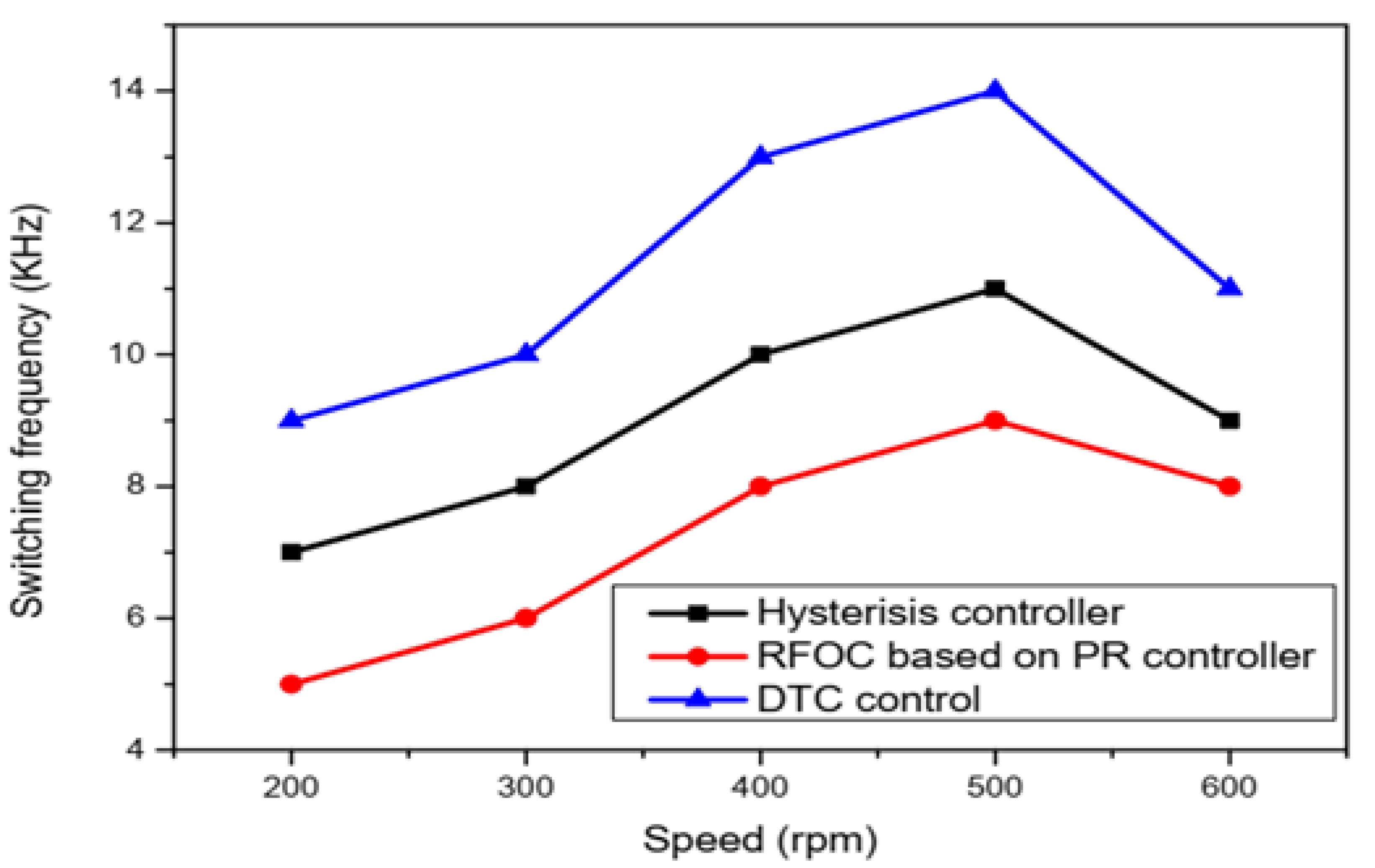
• The presented analysis outlines the features of different control techniques for the FPIM under open phase fault condition and itemize the most suitable one in terms of ripples reduction and switching frequency range.

The paper content is structured so that in Section 2, the characteristics of the five-phase IM drive under the open phase are analyzed. In Section 3, the post-fault control techniques (hysteresis controller, rotor flux oriented control based on PR controller and direct torque control are presented. In Section 4, the test results and a comparative study between the proposed methods are introduced, and finally, the conclusions are introduced in the last section.

2. Characteristic Analysis under Open Phase Fault Condition

The common design of the multi-phase drive system is illustrated in Figure 1. The system consists of two parts: Five-phase VSI supplied with a DC-voltage (V_DC) which can be produced by a DC source or a rectifier. The five-phase IM with symmetrical displacement between two consecutive stator windings equal of 2π = 5 and neutral connection (n). The IGBT or MOSFET switch S₁ is contained in phase ‘a’ in order to contemplate both normal and faulty operations. The modeling and performance of the complete five-phase IM drive system in pre- and post-fault operations are shortly considered in the next subsections.

2.1. Voltage Source Inverter

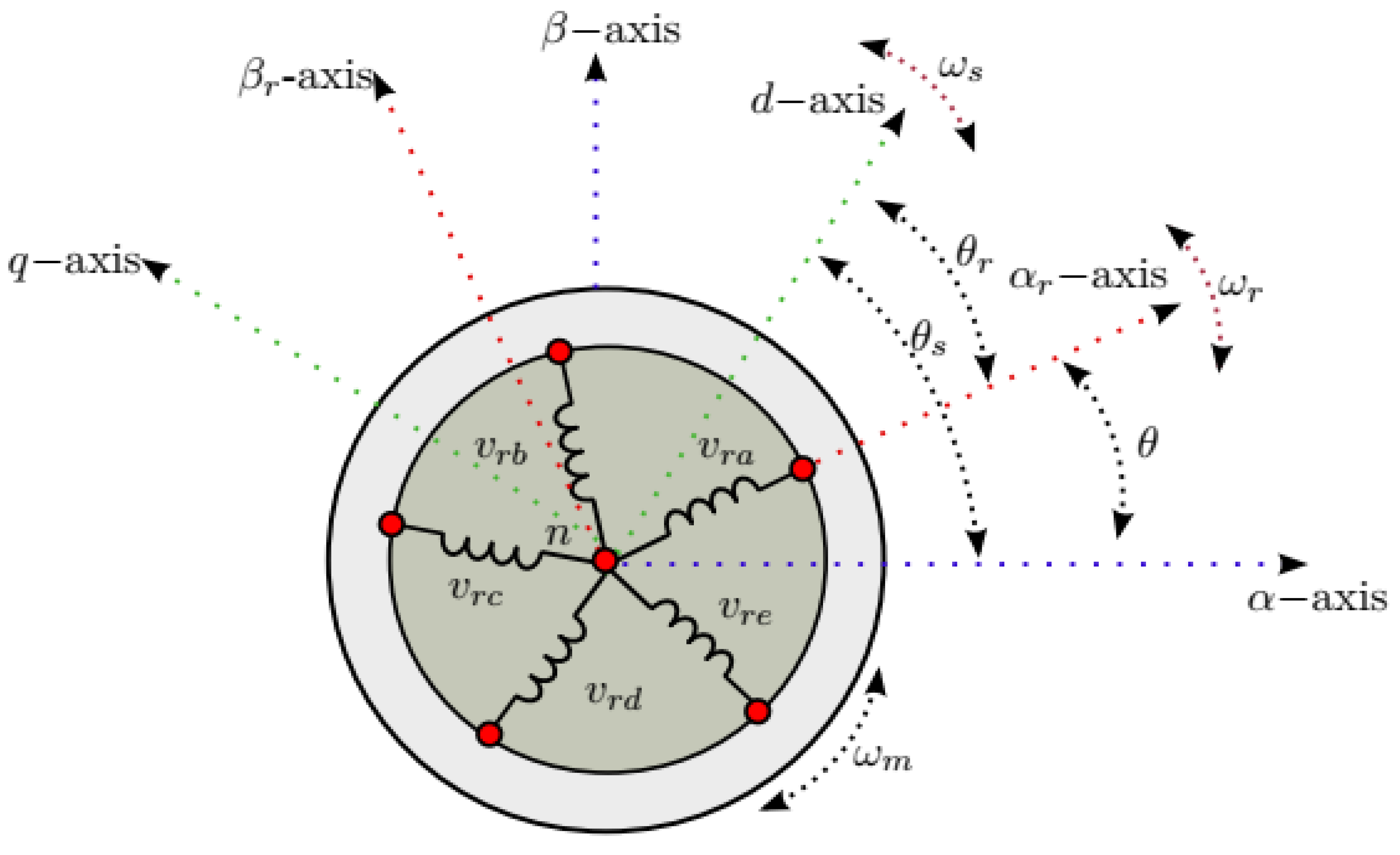
When switch S₁ is closed, the system is now in pre-fault operation and the VSI supplies the five stator windings. The transformation of leg to-phase voltage given as follows:

$$v_{in}=v_{iN}-v_{nN}=S_i{V}_{dc}-v_{nN}.$$

(1)

Assuming the symmetry of the system, then the phase voltage summation is equal to zero (${{\displaystyle \sum }}^{ }{v}_{in}=0$). Moreover, the voltage to neutral (N) is given by:

$$v_{nN}=\frac{V_{dc}}{5}{{\displaystyle \sum }}_{k=a}^e{S}_k,$$

(2)

where as $i\in \left\{a,b,c,d,e\right\}$ refers to the phase. The switching function is designated by S_i for each VSI leg, actually, S_i = 0 if the upper and lower switches are ON and OFF, respectively, and S_i = 1 if the reverse appears. Therefore, by substituting from (2) into (1), the leg-to-phase voltage can be computed in terms of the switching functions by

$$v_{in}=\frac{V_{dc}}{5}\left(4S_i-{{\displaystyle \sum }}_{k=a, k\ne i}^e{S}_k\right)$$

(3)

The leg-to phase voltage can be also represented in a matrix form by

$$\left(\begin{array}{c}{v}_{an}\\ v_{bn}\\ v_{cn}\\ v_{dn}\\ v_{en}\end{array}\right)=\frac{V_{dc}}{5}(\begin{array}{c}4\\ -1\\ -1\\ -1\\ -1\end{array} \begin{array}{c}-1\\ 4\\ -1\\ -1\\ -1\end{array} \begin{array}{c}-1\\ -1\\ 4\\ -1\\ -1\end{array} \begin{array}{c}-1\\ -1\\ -1\\ 4\\ -1\end{array} \begin{array}{c}-1\\ -1\\ -1\\ -1\\ 4\end{array})\left(\begin{array}{c}{S}_a\\ S_b\\ S_c\\ S_d\\ S_e\end{array}\right).$$

(4)

On the opposite, when the switch S₁ in Figure 1 is opened, the system enters the post-fault condition and only the other four phases (b; c; d and e) are still in connection with the VSI. Independently of the fault origination, the open phase current is always zero. Moreover, the available switching states are decreased from 2⁵ = 32 in pre-fault case to 2⁴ = 16 in the faulty condition. Indeed, the Equation (1) is still considered valid in faulty-phase situation; on the contrary, the voltages summation of the unbroken phases is no longer zero and generating an unrestricted oscillation, which cannot be controlled by the neutral voltage. This fact can be expressed by the following equation:

$${{\displaystyle \sum }}_{k=b}^e{v}_{kn}=\frac{-d{\psi }_a}{dt},$$

(5)

where ${\psi }_a$ denotes the flux of the faulty phase (in this case the phase ‘a’) which means that the transformation of leg-to-phase voltage no longer stands on the switching condition, but farther far on the drive operation. Then, the leg-to-phase voltage is calculated by

$$v_{in}=\frac{V_{dc}}{4}\left(3S_i-{{\displaystyle \sum }}_{k=b, k\ne i}^e{S}_k\right)-\frac{d{\psi }_a}{dt}.$$

(6)

By using the matrix form, the leg-to phase voltage becomes,

$$\left(\begin{array}{c}{v}_{bn}\\ v_{cn}\\ v_{dn}\\ v_{en}\end{array}\right)=\frac{V_{dc}}{4}(\begin{array}{c}3\\ -1\\ -1\\ -1\end{array} \begin{array}{c}-1\\ 3\\ -1\\ -1\end{array} \begin{array}{c}-1\\ -1\\ 3\\ -1\end{array} \begin{array}{c}-1\\ -1\\ -1\\ 3\end{array})\left(\begin{array}{c}{S}_b\\ S_c\\ S_d\\ S_e\end{array}\right)-\frac{1}{4}\left(\begin{array}{c}1\\ 1\\ 1\\ 1\end{array}\right)\frac{d{\psi }_a}{dt}.$$

(7)

This final accomplishment has a significant effect on the overall control performance as the reference voltages ($v_{in}^{*}$) are usually determined through regulating the leg voltages ($v_{iN}$) and presuming that the pulse width modulation (PWM) will ensure that $v_{in}=v_{in}^{*}$ on the average value form. However, this is only correct in normal operation via utilizing the transformation procedure in (4). When the leg-to-phase transformation is influenced by the induced back-EMF of the faulted phase (phase ‘a’) as shown in (6), then the voltage becomes $v_{in}\ne v_{in}^{*}$. If one uses the space vector PWM (SVPWM), the space vectors of (3) are no longer right. Rather, if the PWM is chosen as a carrier-based, then the modulation of leg-voltages ($v_{iN}$) can ensure that $v_{iN}=v_{in}^{*}$.

2.2. Five-Phase IM

The motor model can be characterized using the voltage relationships of stator and rotor windings, assuming symmetrical windings’ distribution, sinusoidal (MMF), uniform air gap, and negligible core losses and magnetic saturation. In order to facilitate the control implementation, the use of the phase variable approach is split into two orthogonal subspaces utilizing an adequate transformation. The VSD method permits the modeling of the five-phase IM over an ensemble of four autonomous variables separated into three iso planes, respectively α–β plane, x–y plane, and z term which is zero). A layout for this ensemble is illustrated in Figure 2.

The torque is produced by the harmonic components which are shaped in the α–β plane, otherwise there is no generated torque due to the harmonic components which are shaped in the x–y plane. The general Clarke transformation in healthy condition is given by [38].

$$\left(\begin{array}{c}{v}_{s\alpha }\\ v_{s\beta }\\ v_{sx}\\ v_{sy}\\ v_{sz}\end{array}\right)=\frac{2}{5}\underset{\left[T_5\right] Clarke Matrix under normal Operation}{\underbrace{(\begin{array}{c}1\\ 0\\ 1\\ 0\\ \frac{1}{2}\end{array}\begin{array}{c}\cos \left(\theta \right)\\ \sin \left(\theta \right)\\ \cos \left(2\theta \right)\\ \sin \left(2\theta \right)\\ \frac{1}{2}\end{array} \begin{array}{c}\cos \left(2\theta \right)\\ \sin \left(2\theta \right)\\ \cos \left(4\theta \right)\\ \sin \left(4\theta \right)\\ \frac{1}{2}\end{array} \begin{array}{c}\cos \left(3\theta \right)\\ \sin \left(3\theta \right)\\ \cos \left(\theta \right)\\ \sin \left(\theta \right)\\ \frac{1}{2}\end{array} \begin{array}{c}\cos \left(4\theta \right)\\ \sin \left(4\theta \right)\\ \sin \left(3\theta \right)\\ \sin \left(3\theta \right)\\ \frac{1}{2}\end{array})}}\left(\begin{array}{c}{v}_{an}\\ v_{bn}\\ v_{cn}\\ v_{dn}\\ v_{en}\end{array}\right).$$

(8)

Moreover, the resulted α–β, and x–y voltage relationships can be defined as follows

$${\underset{\_}{v}}_{s\alpha \beta }=\left(R_s+L_s\frac{d}{dt}\right).{\underset{\_}{i}}_{s\alpha \beta }+L_m\frac{d{\underset{\_}{i}}_{s\alpha \beta }}{dt}+L_m\frac{d{\underset{\_}{i}}_{r\alpha \beta }}{dt}$$

(9)

$$0=\left(R_r+L_r\frac{d}{dt}\right).{\underset{\_}{i}}_{r\alpha \beta }+L_m\frac{d{\underset{\_}{i}}_{s\alpha \beta }}{dt}-j{\omega }_r.\left(L_m{\underset{\_}{i}}_{s\alpha \beta }+L_r{\underset{\_}{i}}_{r\alpha \beta }\right)$$

(10)

$${\underset{\_}{v}}_{sxy}=\left(R_s+L_{ls}\frac{d}{dt}\right).{\underset{\_}{i}}_{sxy}.$$

(11)

The underlined variables pertain to the complex variables, ${\omega }_r$ denotes the electrical rotor speed. The set of Equations (8) and (9) permits the calculation of the back-EMF of the open phase as given by (12), this value is mandatory to evaluate (6):

$$\frac{d{\psi }_a}{dt}=L_m\left(\frac{d{i}_{s\alpha }}{dt}+\frac{d{i}_{r\alpha }}{dt}\right).$$

(12)

Using (12), Equation (7) can be rewritten as:

$$\left(\begin{array}{c}{v}_{bn}\\ v_{cn}\\ v_{dn}\\ v_{en}\end{array}\right)=\frac{V_{dc}}{4}(\begin{array}{c}3\\ -1\\ -1\\ -1\end{array} \begin{array}{c}-1\\ 3\\ -1\\ -1\end{array} \begin{array}{c}-1\\ -1\\ 3\\ -1\end{array} \begin{array}{c}-1\\ -1\\ -1\\ 3\end{array})\left(\begin{array}{c}{S}_b\\ S_c\\ S_d\\ S_e\end{array}\right)-\frac{1}{4}\left(\begin{array}{c}1\\ 1\\ 1\\ 1\end{array}\right).L_m\left(\frac{d{i}_{s\alpha }}{dt}+\frac{d{i}_{r\alpha }}{dt}\right).$$

(13)

During the fault period, the VSD method can be formulated in two different ways. The first is to maintain the use of the pre-fault transformation defined by (7). This is the easy way to regulate the current due to the fact that the open phase current is popular to be zero ($i_{s\alpha }=0$), so the other currents can be directly evaluated. It must be recognized that the five VSD currents are no more separate as in the normal situation, therefore, the faulty-phase condition must be fulfilled through making ($i_{sx}=-i_{s\alpha }$). The VSD model represented in (9) and the α–β reference currents, as in pre-fault operation are still circular. Actually, if the VSD is used for the voltage control, it is impossible to control the back-EMF which makes the application of (7) very difficult. The second alternative concerns with using the Clarke transformation with reduced order to prevent the use of open phase current/voltage. This alternative has been developed respectively in [6,39] for two types of multi-phase drives. However the transformation matrix is maintained from the point of view of orthogonality, but at the end, the α–β steady-state reference current components became ellipsoidal. Moreover, the drive parameters became time-dependent. Indeed, using the reduced-order transformation from (8) makes it possible to derive the nonorthogonality, thus the model in the healthy situation of (9) is useful in this case. After all, the faulty phase back-EMF is equivalent to the minus of the healthy voltage summation ($\frac{d{\psi }_a}{dt}=-{{\displaystyle \sum }}_{i=b}^e{v}_{in}$), then it is easy to exclude the x-term in (7) and representing the matrix as follows:

$$\left(\begin{array}{c}{v}_{s\alpha }\\ v_{s\beta }\\ v_{sy}\\ v_{sz}\end{array}\right)=\frac{2}{5}\underset{\left[T_4\right] Clarke Matrix in Faulty Operation}{\underbrace{(\begin{array}{c}\cos \left(\theta \right)-1\\ \sin \left(\theta \right)\\ \sin \left(2\theta \right)\\ 1\end{array} \begin{array}{c}\cos \left(2\theta \right)-1\\ \sin \left(2\theta \right)\\ \sin \left(4\theta \right)\\ 1\end{array} \begin{array}{c}\cos \left(3\theta \right)-1\\ \sin \left(3\theta \right)\\ \sin \left(6\theta \right)\\ 1\end{array} \begin{array}{c}\cos \left(4\theta \right)-1\\ \sin \left(4\theta \right)\\ \sin \left(8\theta \right)\\ 1\end{array})}}\left(\begin{array}{c}{v}_{bn}\\ v_{cn}\\ v_{dn}\\ v_{en}\end{array}\right)$$

(14)

The back-EMF of the faulty-phase is discursively incorporated in the first row of (14). Then, by using the Clarke-transformation [T₅] of (8) or the reduced-order transformation [T₄] of (14), the system model in the post-fault situation maintains the same behavior as in the pre-fault stat, and the reference values of α–β currents remain circular. The characteristics of the VSI and five-phase motor can be summarized in

Table 1. Characteristics of five-phase IM drive in pre-fault and post-fault operation.

Characteristics of Five-Phase IMdrive System	Pre-Fault Operation	Post-Fault Operation
Possible switching states	25 = 32	24 = 16
Leg-to-phase voltages	Equations (3) and (4)	Equations (6), (7) and (13)
Clarke transformation	Matrix [T5]	Matrix [T4]
Motor model	Equations (8) and (9)	Equations (14) and (9)

, in which a brief comparison is presented.

2.3. Post-Fault Current Reference Calculation

For the post-fault operation, several control topologies can be used according to the application. Recently, different controllers are designed to guarantee minimal derating, limited Joule losses, or minimal torque fluctuations [2,11]. Based on the preferred control methodology, the permissible limits of α–β currents can be varied; thus the reference currents in the x–y trajectory have to be adjusted to guarantee stable dynamics. For comparison purpose, this paper contemplates both criteria’s minimum derating (MD) and minimum losses (ML) as stated in the following subsections:

2.3.1. Minimum Derating (MD)

The main requirement in the post-fault operation is to maximize the production of the torque, which can be achieved when the RMS current values of the healthy windings are equal, which changes the calculation of ‘y’ current component to be as following:

$$\{\begin{array}{c}{i}_{sb}=-i_{sd},i_{sc}=-i_{se}\\ i_{sy}^{*}=\frac{\sin \left(\theta \right)-\sin \left(2\theta \right)}{\sin \left(\theta \right)+\sin \left(2\theta \right)}.i_{s\beta }^{*}=-0.2631.i_{s\beta }^{*}\end{array}$$

(15)

Taking into account the motor ratings, the reference currents representation in the α–β plane can be defined by:

$$\{\begin{array}{c}{i}_{s\alpha }^{*max}=0.7236.I_n.\sin \omega t\\ i_{s\beta }^{*max}=-0.7236.I_n.\cos \omega t\end{array}$$

(16)

2.3.2. Minimum Copper Losses (ML)

The mechanism of minimizing the copper losses is adopted to enhance the drive efficiency. The reference currents in the subspace α–β are computed in that manner which aims to improve the torque/flux regulation. In this manner, the reference of the y-current component is kept to zero ($i_{sy}^{*}=0$) since the y-component is not responsible for torque production. This method ensures high efficiency and allows the minimization of the losses; this is generalized by unequal peak current values of the motor phases [11]. The drive requires the derating process in order to keep the currents in the un faulted phases to the rated value (I_n). Therefore, via considering the maximum rated values and maintaining a rotating circular-shaped MMF, the reference currents waveforms defined in the α–β subspace can be expressed by:

$$\{\begin{array}{c}{i}_{s\alpha }^{*max}=0.6813.I_n.\sin \omega t\\ i_{s\beta }^{*max}=-0.6813.I_n.\cos \omega t\end{array}$$

(17)

3. Post-Fault Control Techniques and Comparative Study

3.1. Hysteresis Regulators

Several studies adopted the utilization of hysteresis-based regulators, considering the advantages of such controllers, such as the high bandwidth and the ability to observe the post-fault reference currents’ oscillations. However, the variable switching frequency of such controllers makes the implementation very difficult in certain applications. A controller example is presented in Figure 3. The scheme is constructed from an external speed-loop that develops the necessary torque command, a current reference generator which is designed considering several fault types and an internal current-loop followed by a hysteresis controller proposed to track the optimal reference currents. Afterwards, the torque reference and the fault information are fed to the block of the optimum reference current generation, which selects the adequate lookup table. It is clear that the selected reference values (saved in look-up tables), are not computed online, however, they are computed off-line using the reference torques and the corresponding back-EMF.

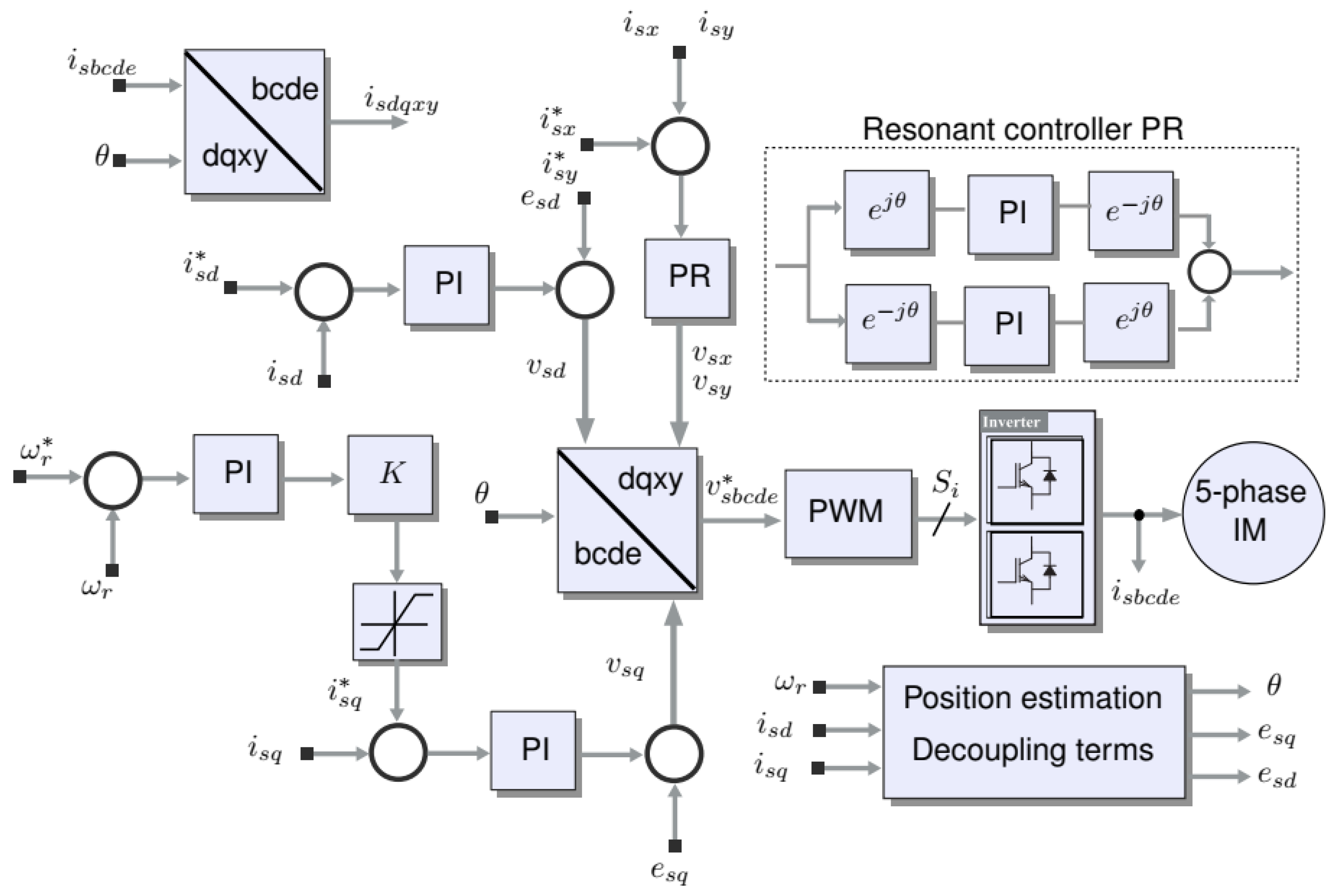
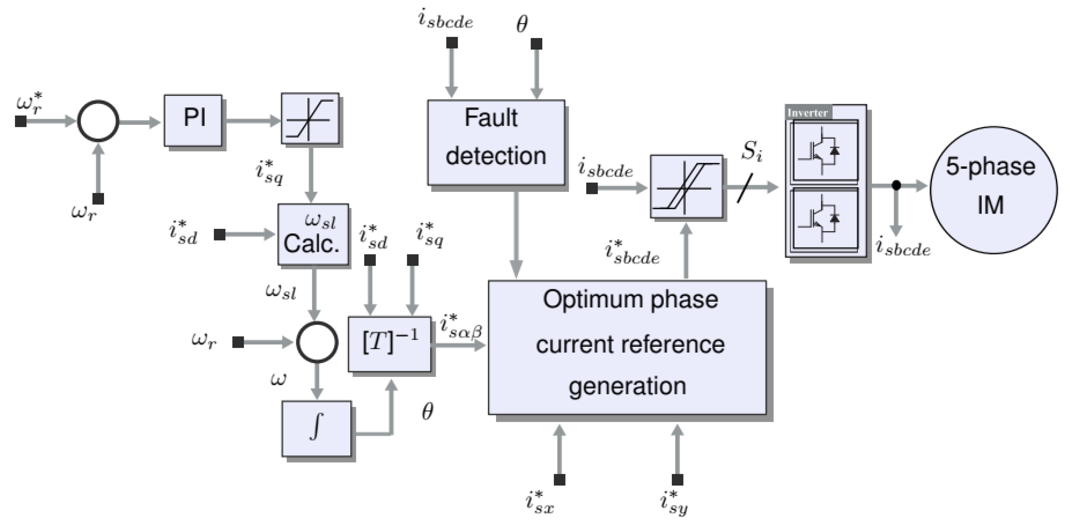
3.2. Field Oriented Control Using Resonant Controller

The second control configuration utilizes a speed controller with conventional PI and PI resonant controllers. Both PI and PR regulators are used extensively for obtaining a better steady-state dynamic [40]. The layout of the implemented controller is illustrated in Figure 4. The resonant controller is designated as PR in the following sections. Under field orientation, the control system defined in the d-q rotating plane is implemented using the traditional PI regulators and the speed controller with anti-windup. The reference d-current component is kept to a fixed value, while the q-component is calculated by the PI speed regulator, this is performed using the hysteresis controller illustrated in Figure 3. Hence, only the current regulation is required. The voltage space decomposition (VSD) in the α–β–d–q spaces is accomplished using the classic Clarke matrix [T₅] given by (8). For the hysteresis controller, the d–q currents are shaped into the α–β space using (18), while the angular displacement is calculated indirectly using (20).

$$\left(\begin{array}{c}{\mathit{i}}_{\mathit{s}\mathit{\alpha }}^{*}\\ {\mathit{i}}_{\mathit{s}\mathit{\beta }}^{*}\end{array}\right)=\underset{\left[{\mathit{T}}_{\mathit{e}\mathit{q}}\right] Park Matrix}{\underbrace{\left(\begin{array}{cc}\mathbf{cos}\mathit{\theta }& -\mathbf{sin}\mathit{\theta }\\ \mathbf{sin}\mathit{\theta }& \mathbf{cos}\mathit{\theta }\end{array}\right)}}.\left(\begin{array}{c}{\mathit{i}}_{\mathit{s}\mathit{d}}^{*}\\ {\mathit{i}}_{\mathit{s}\mathit{q}}^{*}\end{array}\right).$$

(18)

The main variation compared with the hysteresis regulator is that the inner adaptation loops for the d–q and x–y components are performed using the PI and PR regulators. Moreover, in the pre-fault case, the α–β–x–y reference voltages are calculated using regular decoupling terms $e_{sd}$ and $e_{sq}$ for the sake of enhancing the controller performance:

$$\{\begin{array}{c}{e}_{sd}=\sigma L_s{i}_{sq}^{*}{\omega }_r\\ e_{sq}=L_s\frac{{\psi }_r^{*}}{L_m}{\omega }_r\end{array}$$

(19)

$$\theta ={{\displaystyle \int }}^{ }\left({\omega }_r+{\omega }_{sl}\right)dt={{\displaystyle \int }}^{ }\left({\omega }_r+\frac{L_m{i}_{sq}^{*}}{{\tau }_r{\psi }_r^{*}}\right)dt$$

(20)

The VSD reference voltages are lastly converted into phase reference voltages utilizing [T₅] and relocated to the PWM level, which in this work is carrier-based. For normal operation, with fixed d–q and zero x–y reference currents, the PI regulators are validated to achieve an acceptable investigation for the reference signals. Nevertheless, the x–y current components in post-fault operation have an oscillating component by nature, thus using the classic PI controllers accompanied by limited bandwidth does not allow accordingly tracking the reference currents. So, the reference x–y terms are regulated over a combination of PR regulators which are able to follow the oscillated currents. In Ref. [41], the PR regulator is formed of two PI controllers applied in two rotating frames, for the sake of precise tracking of both negative and positive sequence currents. Every PI regulator is able to converge the input error to zero. Therefore, the summation of both outputs forms the PR as shown in Figure 4.

The tuning process of the PR regulator can be described according to the following procedure:

The PI regulator performs two processes and combines them to construct the reference signals to be subjected to the plant under study. This process can be mathematically expressed by

$$U\left(s\right)=U_p\left(s\right)+U_i\left(s\right),$$

(21)

where $U_p\left(s\right)$ is the proportional term and $U_i\left(s\right)$ is the integral component. These terms can be expressed by

$$U_p\left(s\right)=k_p\left(s\right)E\left(s\right), \mathrm{and} U_i\left(s\right)=\frac{k_i\left(s\right)}{s}E\left(s\right).$$

(22)

$E\left(s\right)$ is the input error signal to the regulator. Then, the PI’s transfer function can be expressed by

$$H_{pi}\left(s\right)=\frac{U\left(s\right)}{E\left(s\right)}=k_p+\frac{k_i}{s}=k_p{C}_p\left(s\right)+k_i{C}_i\left(s\right).$$

(23)

The main task of the PI regulator is to ensure zero deviation between the reference and actual controlled signals. This can be solely accomplished via the integral component of the regulator, meanwhile, the proportional term is null under steady-state operation. So, it can be said that the integral term is the dominant of the regulator’s dynamics; even it can be utilized alone to achieve the control target. In general, any process that has stable behavior can be regulated using a pure integral regulator combined with a simple integral gain. However, for the transient operation, the performance when using only the integral part significantly degrades. For this reason, the proportional term is added to the integral to improve the dynamics during the transient conditions and to enhance the robustness of the closed-loop system. The proportional effect is considered as the derivative of the integral part, so

$$C_p\left(s\right)={sC}_i\left(s\right).$$

(24)

3.2.1. The PR Regulator Structure

When considering a variable reference type (such as sinusoids with constant frequency ${\omega }_r$), and in order to track them and restrict the external disturbances, the resonant regulator can be used to fulfill these requirements. The action taken by the PR can be described by

$$C_r\left(s\right)=\frac{s}{s^2+{\omega }_r^2},$$

(25)

where ${\omega }_r$ is the frequency that needs to be tracked or rejected. The integral action $C_i\left(s\right)$ can be considered as a special case of the resonant action of (25), which can be obtained via putting ${\omega }_r=$ 0.0.

Similar to the fixed reference case, extra control processes should be incorporated to satisfy the proper dynamic operation. To describe the extra provided action, the same principle which is adopted with the PI expressed by (24) will be considered here. Then, by calculating the derivative of resonant term, results in

$$C_p\left(s\right)={sC}_r\left(s\right).$$

(26)

This component is then added to resonant action to get finally the relationship which describes the PR regulator’s operation as follows

$$C_{pr}\left(s\right)=k_p\frac{s}{s^2+{\omega }_r^2}+k_r\frac{s}{s^2+{\omega }_r^2},$$

(27)

where $k_p$ and $k_r$ are the regulator’s gains to be determined via tuning.

3.2.2. Tuning of PR Regulators

In Ref. [42], a tuning mechanism entitled forced oscillation method (FOM) was presented, based on causing an oscillation in a closed-loop, then the amplitude and frequency of the oscillations are measured and after that, the method introduced simple formulas for each regulator parameter; these formulas contain the measured variables. In the current paper, the FOM is utilized to tune the PR regulators as follows

The FOM technique depends on the identification of the ultimate value of the plant’s frequency-based response. The ultimate value for any frequency response is the value obtained at a position where the Nyquist plot of the response passes the negative real axis, which also refers to the point related to the minimum frequency for which the phase margin get the value of −π. The specifications of the ultimate value/point are the ultimate gain $k_u$ and ultimate frequency ${\omega }_u$ which can be expressed by

$$k_u=\frac{1}{\left|G\left(j\omega \right)\right|}$$

(28)

$${\omega }_u=\underset{\omega \ge 0}{\underbrace{min}} \omega : \angle G\left(j\omega \right)=-\pi .$$

(29)

With these relationships, the operation mechanism of the FOM can be itemized as follows:

(a)

Ultimate points for the frequency ${\omega }_u$ and gain $k_u$ are firstly determined.

(b)

The regulator parameters are selected such that

$$C\left(j{\omega }_u \right)G\left(j\omega \right)=p, \mathrm{or} C\left(j{\omega }_u \right)=-k_{u}p,$$

(30)

where p is a specified position in the complex s-plane.

Now for the PR regulator, the frequency response can be described by

$$C\left(j\omega \right)=\frac{j{k}_r\omega -k_p{\omega }^2}{{\omega }_r^2-{\omega }^2}.$$

(31)

Replacing from (31) into (30) yields

$$\frac{j{k}_r{\omega }_u-k_p{\omega }_u^2}{{\omega }_r^2-{\omega }_u^2}=-k_{u}Re\left(p\right)-j{k}_{u}Im\left(p\right),$$

(32)

where $Re$ and $Im$ are the real and imaginary terms of p.

Then from (32), the regulator’s gains can be separated as follows

$$k_p=k_{u}Re\left(p\right)\frac{{\omega }_r^2-{\omega }_u^2}{{\omega }_u^2}, \mathrm{and} k_r=k_{u}Im\left(p\right)\frac{{\omega }_u^2-{\omega }_r^2}{{\omega }_u}.$$

(33)

After the proper tuning of the regulator, the controller structure will be able to drive the total tracking error to zero. From (5), the neutral-voltage oscillation is obviously considered in the vector control technique using (6) and (13), and so it needs to be compensated indirectly in the PR control by the linear current controllers. For the PR, it is mandatory to set an x-reference current ensuring that ($i_{sx}=-i_{s\alpha }$) to avoid an incompatible response from the x and α regulators. The designed PR controller limits the needed arrangements when the drive changes its operating point (from pre to post-fault situations). The principal actions that must be set in motion after the fault detection are:

• The PI regulators which are used in the x–y frame must be resonant regulators and their parameters must be adjusted.
• The y-reference current must be replaced, according to the applied control in the post-fault operation, either to ($i_{sy}^{*}=0$) for minimum losses or to (15) for minimum deration.
• The limitations for the α–β currents changes have to be modified according to either (17) for minimum losses or to (16) for minimum deration; this action can be realized through modifying the saturation limits of the anti wind-up PI current controllers.

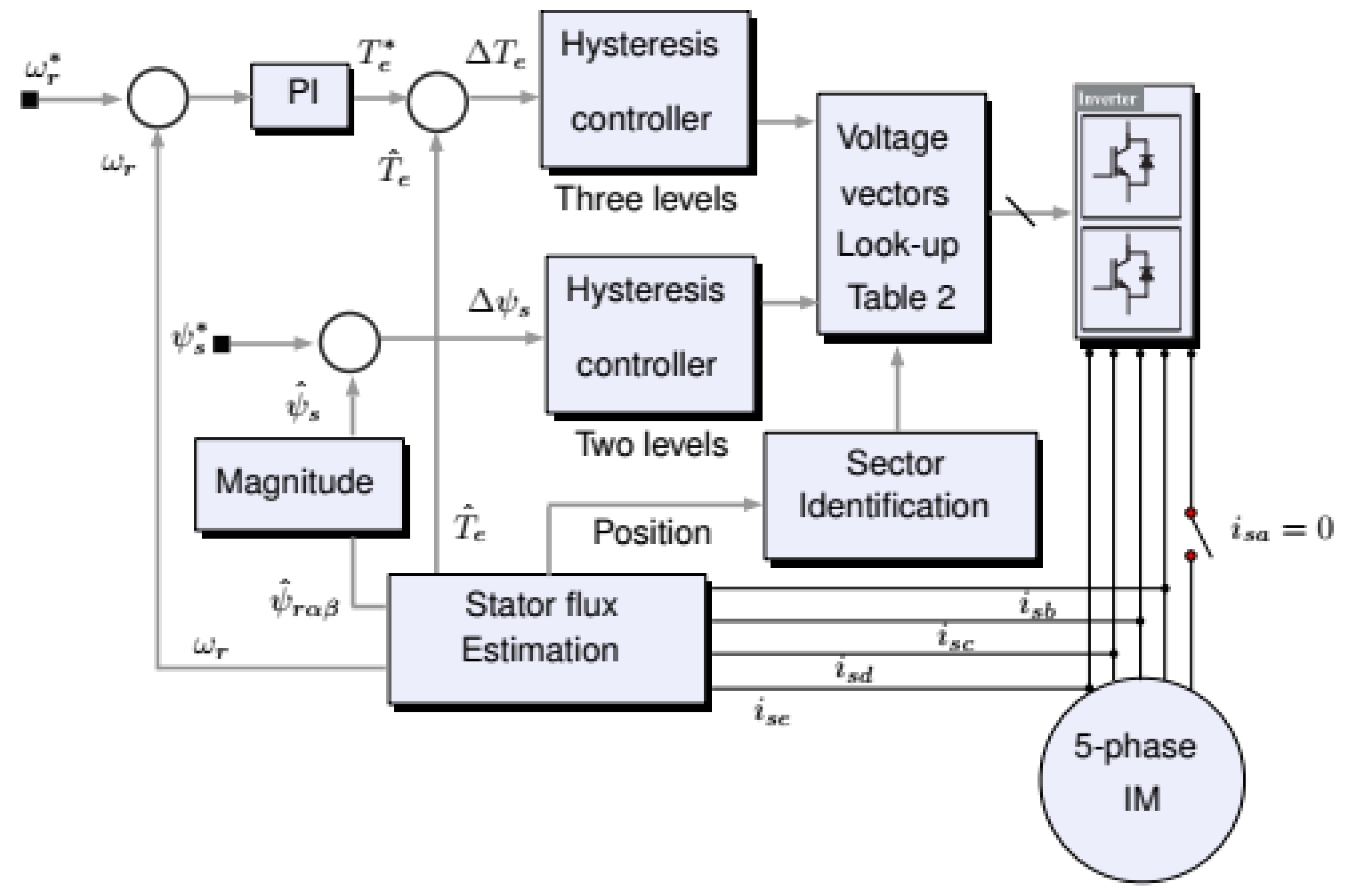
3.3. Post Fault Direct Torque Control

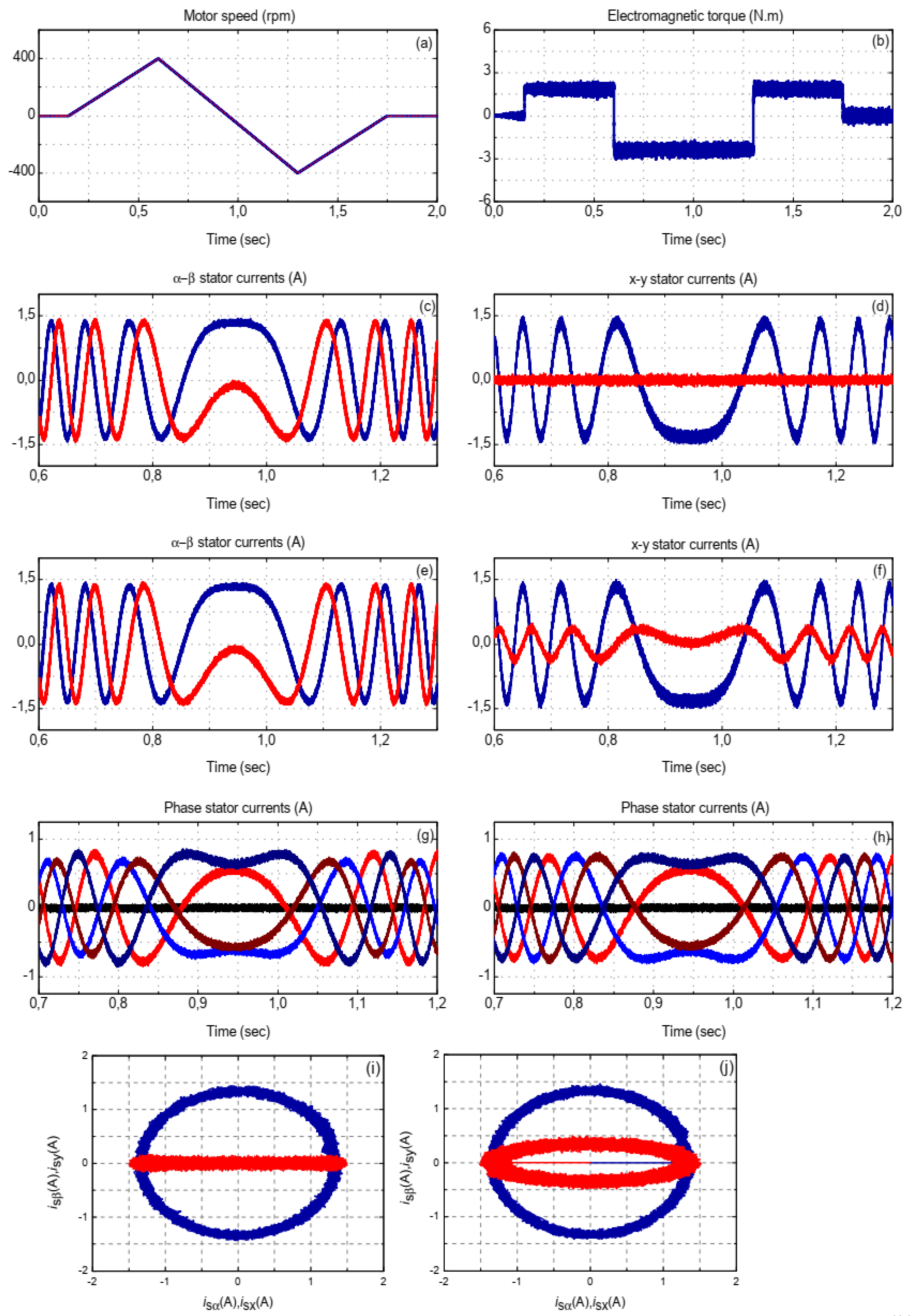
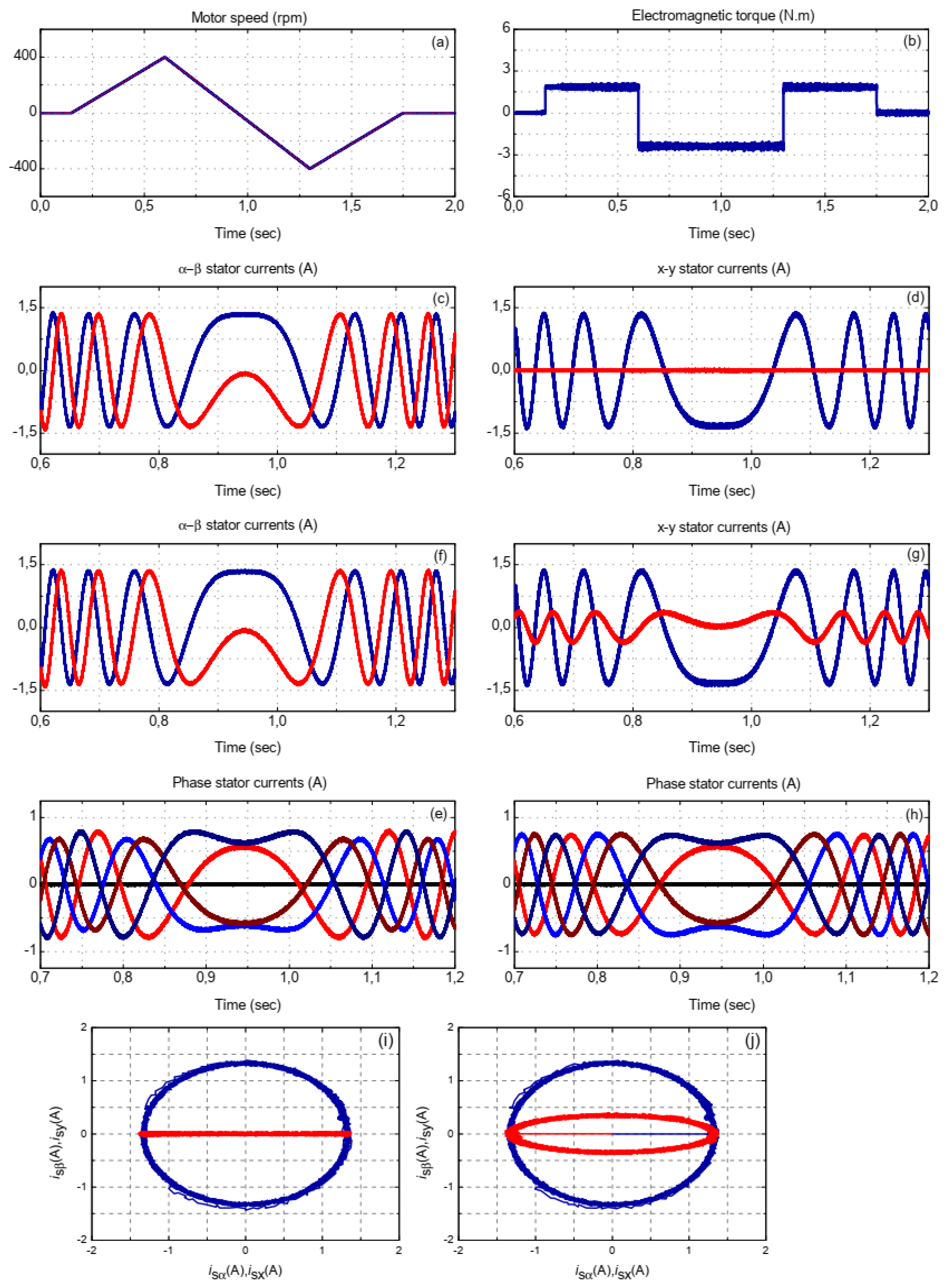
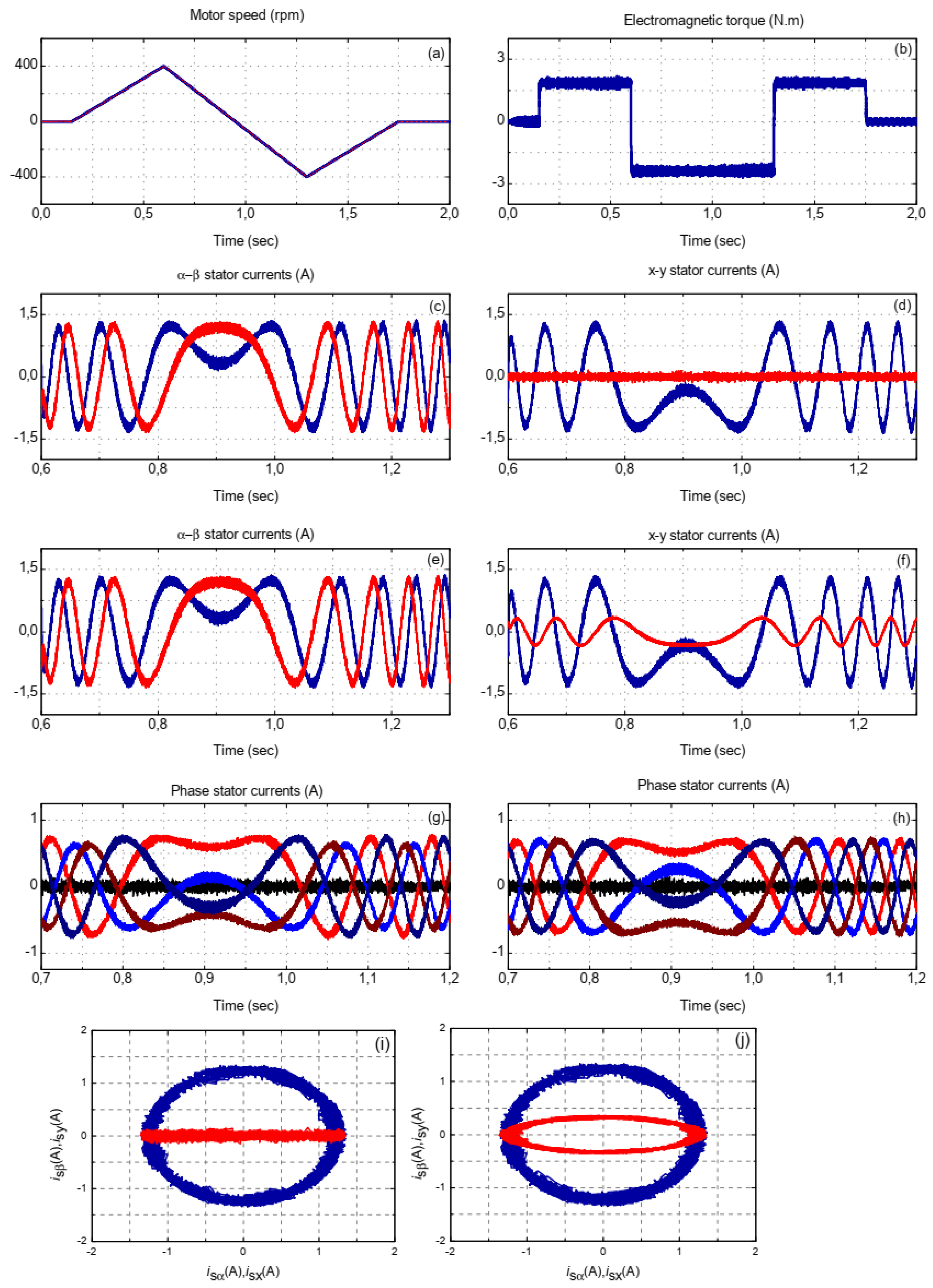
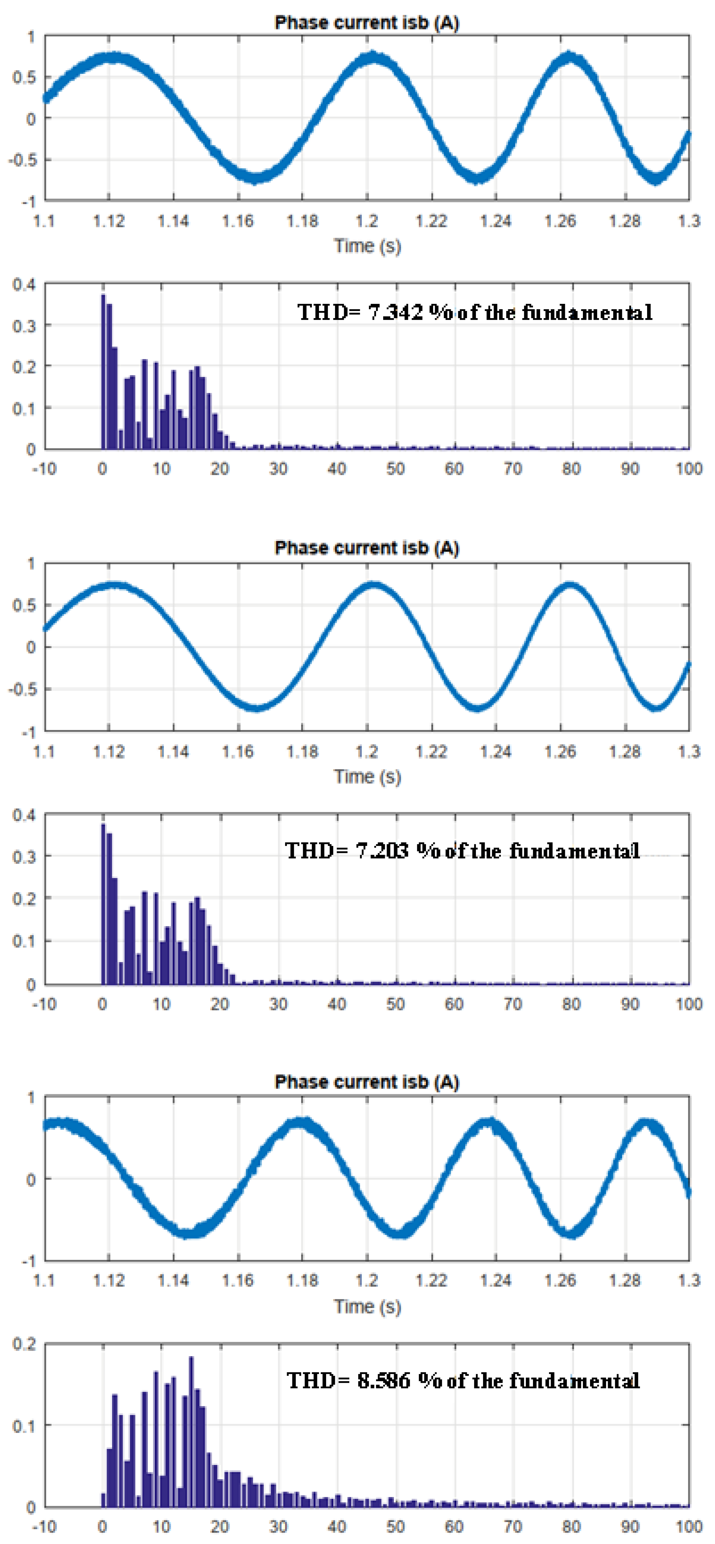
The DTC control configuration depends on ten dynamic virtual vectors which are located in the α–β frame. The dynamic virtual vector is implemented depending on the estimated flux, the developed torque and the sector of the flux vector, and two comparators with hysteresis-based operation. Moreover, the virtual voltage vector is accomplished by a mix of voltage vectors with different sizes located in the α–β frame with an adequate dwell time to induce zero volts/seconds in the x–y space. The vectors in the α–β frame must induce the reverse in the stage of medium and small vectors in the x–y trajectory, so the standardized dwell times designated to a sampling interval T_s are $K_{vr}=\left(3-\sqrt{5}\right)/2$ and $1-K_{vr}$, separately, and the incorporated virtual voltages have an amplitude of $\left(\left(5-\sqrt{5}\right)/2\right)*V_{dc}$. The control type to be considered for the post-fault operation must be similar to the pre-fault state. In fact, the voltage vectors number in α–β and x–y frames is varied. While 32 vectors turn out in the normal condition, there will be only 16 vectors are available in the post-fault, as shown in Figure 5.

Accordingly, the virtual voltages set described in Ref. [43] are no more valid and a new set has to be formulated to be utilized during the fault period. The flux deviation $\left(∆{\psi }_s\right)$ between the reference $\left({\psi }_s^{*}\right)$ and estimated $\left({\widehat{\psi }}_s\right)$ fluxes is applied to a hysteresis regulator with two levels which generate (+1) to raise the flux and (0) to decrease it. The torque regulator develops (+1) to raise the torque, and (−1) to decrease it and (0) to maintain it fixed to a selected reference value. Using an extra number of hysteresis levels enables limiting the inverter switching frequency, as the flux dynamics are commonly slower than the torque variation. The switching states determine the sequential operation of the VSI (see

Table 2. Dwell times during the fault.

Dwell Time	Virtual Vectors
	${\mathit{V}}_1\left(9\right)$	${\mathit{V}}_2\left(13,8\right)$	${\mathit{V}}_3\left(10,12\right)$	${\mathit{V}}_4\left(4,14\right)$	${\mathit{V}}_5\left(6\right)$	${\mathit{V}}_6\left(2,7\right)$	${\mathit{V}}_7\left(5,3\right)$	${\mathit{V}}_8\left(11,1\right)$
$K_{vr1}$	1	0.382	0.191	0.382	1	0.382	0.191	0.382
$K_{vr2}$	-	0.618	0.809	0.618	-	0.618	0.809	0.618

). The vector $V_k$ is the actual applied vector, while the indices k − 1 and k + 1 refer to the nearby sectors (pre and post sectors). This selection is performed according to the torque and flux errors ($∆T_e$ and $∆{\psi }_s$), and on the stator flux angle (sector $s_i$ (i = 1,2,…,8)). This is the result of losing one degree of freedom due to the fault, where a defined relation between $\alpha$ and x coordinates results in the threshold of $i_{sx}=-i_{s\alpha }$. The remaining degree of freedom is appropriate to maintain zero volts/seconds in the y axis. Thus, by limiting the y-current, eight virtual vectors ($V_k$) defined in the α–β space are available (see Figure 6, in which each $V_k$ is positioned in the sector’s center and outlined by dashed lines and remarked by different numbers). Actually $K_{vr1}$ and $K_{vr2}$ are the dwell time ratios which calculate $V_k$ in terms of two permissible vectors ($V_1$ and $V_2$).

$$V_k\left(V_1,V_2\right)=K_{vr1}{V}_1+K_{vr2}{V}_2$$

(34)

Various time ratios are now proposed in comparison with the pre-fault drive operation (see Table 2).

The recommended post-fault DTC approach is characterized in Figure 7.

Table 3. Post-fault operation look-up table.

$\mathbf{∆}{\mathit{\psi }}_{\mathit{s}}$	$\mathbf{∆}{\mathit{T}}_{\mathit{e}}$	Stator Flux Sector
		1	2	3	4	5	6	7	8
+1	+1	${\mathit{V}}_2$	${\mathit{V}}_3$	${\mathit{V}}_4$	${\mathit{V}}_5$	${\mathit{V}}_6$	${\mathit{V}}_7$	${\mathit{V}}_8$	${\mathit{V}}_1$
	−1	${\mathit{V}}_8$	${\mathit{V}}_1$	${\mathit{V}}_2$	${\mathit{V}}_3$	${\mathit{V}}_4$	${\mathit{V}}_5$	${\mathit{V}}_6$	${\mathit{V}}_7$
	0	${\mathit{V}}_0$	${\mathit{V}}_9$	${\mathit{V}}_0$	${\mathit{V}}_9$	${\mathit{V}}_0$	${\mathit{V}}_9$	${\mathit{V}}_0$	${\mathit{V}}_9$
−1	+1	${\mathit{V}}_4$	${\mathit{V}}_5$	${\mathit{V}}_6$	${\mathit{V}}_7$	${\mathit{V}}_8$	${\mathit{V}}_1$	${\mathit{V}}_2$	${\mathit{V}}_3$
	−1	${\mathit{V}}_6$	${\mathit{V}}_7$	${\mathit{V}}_8$	${\mathit{V}}_1$	${\mathit{V}}_2$	${\mathit{V}}_3$	${\mathit{V}}_4$	${\mathit{V}}_5$
	0	${\mathit{V}}_9$	${\mathit{V}}_0$	${\mathit{V}}_9$	${\mathit{V}}_0$	${\mathit{V}}_9$	${\mathit{V}}_0$	${\mathit{V}}_9$	${\mathit{V}}_0$

specifies the modified virtual vectors, which are configured according to the hysteresis limits, the $∆T_e$ and $∆{\psi }_s$ errors and the flux sector.

In the DTC scheme, the reference torque signal ($T_e^{*}$) is developed using a PI speed regulator, while the flux command (${\psi }_s^{*}$) is set to its rated value, as under normal DTC operation, this is due to the drive rotating at its rated speed.

4. Results

The five-phase IM drive performance is tested with three different control approaches; Hysteresis controller, RFOC based on the PR controller and DTC control technique. The Data specifications for the system under study are summarized in

Table A1. Parameters of five-phase IM drive system.

Parameters	${\mathit{R}}_{\mathit{s}}$	${\mathit{R}}_{\mathit{r}}$	${\mathit{L}}_{\mathit{s}}$	${\mathit{L}}_{\mathit{r}}$	${\mathit{L}}_{\mathit{l}\mathit{s}}$	${\mathit{L}}_{\mathit{l}\mathit{r}}$	${\mathit{L}}_{\mathit{m}}$	P	${\mathit{T}}_{\mathit{e}\mathit{n}}$	${\mathit{I}}_{\mathit{n}}$	${\mathit{\psi }}_{\mathit{s}\mathit{n}}$	${\mathit{J}}_{\mathit{m}}$
Value	10	6.3	0.46	0.46	0.04	0.04	0.42	2	8.33	2.1	1.2705	0.01

and

Table A2. Data of controllers.

PI Gains		PR Gains		DTC		Hysteresis Controller
${\mathit{K}}_{\mathit{p}}$	${\mathit{K}}_{\mathit{i}}$	${\mathit{K}}_{\mathit{p}}$	${\mathit{K}}_{\mathit{r}}$	Flux Comparator Limits	Torque Comparator Limits	Hysteresis Limits
7.5398	2842.4	2000	0.1	0.007 and −0.007	0.005 and −0.005	$\pm$2 * ${\mathit{I}}_{\mathit{n}}$

in Appendix A.

Figure 8, Figure 9, Figure 10, Figure 11 and Figure 12 summarize the results for the hysteresis controller, RFOC and DTC control, where a DC link voltage V_dc of 300 V was used. Figure 8 presents the results of the first control technique, where the motor drives under a triangular reversal speed response from 400 rpm to −400 rpm. Figure 8a–j show respectively the motor speed, electromagnetic torque, the (α–β) stator current in case of ML criteria, the (x–y) stator current in case of ML criteria, the (α–β) stator current using the MD criteria, the (x–y) stator current in case of MD criteria, the phase stator currents using the ML criteria, the phase stator currents using the MD criteria and finally the trajectories of the stator currents (α–β) and (x–y) in both case of ML and MD. As can be noticed from the results, the actual speed tracks definitely its reference value without overshooting, which clarifies the validity of the hysteresis controller in achieving the control targets. However, the presence of inevitable currents and torque ripples due to the use of the hysteresis controller is still the main drawback of such controllers.

Although similar responses are obtained using the RFOC based on PR controller which are detailed in Figure 9a–j, the RFOC generates negligible overshoots and high performance in tracking response and also offers an advantage compared to the hysteresis controller concerning currents and torque ripples. Figure 10a–j illustrate the results of the DTC controller. It is shown that the ripples are obvious compared with the other two controllers. The results report that a good tracking response and high dynamic are achieved but the ripples are still remarkable due to the use of hysteresis controllers. The figures also illustrate the stator currents profiles which are obtained using the hysteresis regulators, RFOC and DTC under the fault condition and when the speed is reversed from −400 to 400 rpm. Figure 11 show the stator flux dynamics under the three control techniques. It is very obvious that the PR controller exhibits the minimum flux ripples while the hysteresis regulator presents the worst performance. From these figures, it can be concluded that the PR controller presents the optimal performance.

For the three control systems, the DTC has the worst performance. It is noticed that the current ripples are much higher than the values obtained in the other two tests. Finally, the spectrum analysis of the phase current b for the three techniques is presented in Figure 12 and every spectrum is followed by the harmonic distortion value THD.

Torque and current ripple obtained for hysteresis controller, PR controller and DTC are presented for different speeds in

Table 4. Currents and torque ripples for different speed range for the three proposed control techniques.

Method	Speed (rpm)	Current Ripple (A)	Torque Ripple (Nm)
Hysteresis controller	100 400	0.12 0.1	0.9 0.7
PR controller	100 400	0.08 0.05	0.7 0.4
DTC controller	100 400	0.24 0.14	1.2 0.8

. Figure 13 illustrates the switching frequencies for different operating speeds while loading the motor with 2 Nm. The switching frequencies are calculated for a time period of t = 0.05 s by recording the switching actions of the inverter. The results show that the proposed RFOC which utilizes a PR regulator presents the minimum switching frequency, while the DTC presents the highest switching frequency for the same conditions. Meanwhile, the proposed hysteresis controller offers an intermediate switching frequency.

Corresponding to the validity of the three controllers in keeping the motor’s operation under the open phase fault condition, it is shown that the three controllers are able to maintain the normal operation of the motor even with an open stator phase, however, the differences between the procedures came into account in terms of torque and current ripples.

5. Conclusions

The paper presented a detailed comparative analysis for the dynamic performances of three control topologies for the five-phase IM under open-phase fault conditions. The specified techniques are the DTC, hysteresis controller and the RFOC. The comparison is carried out in terms of the torque and current ripples and in terms of switching frequency as well. The obtained results demonstrated that the DTC technique has the capability to manage lower maximum electrical torques than the hysteresis controller and RFOC methods. However, by applying the DTC control, the presence of a higher harmonic content is obvious in both stator phase current and torque. While the RFOC PR-based controller has the best performance with the minimum torque and current ripples and switching frequency as well.

References

1. Hang, C.; Emil, L.; Martin, J.; Mario, D.; Wooi, H.; Nasrudin, A. Operation of a six-phase induction machine using series-connected machine-side converters. IEEE Trans. Ind. Electron. 2014, 61, 164–176. [Google Scholar]
2. Jen, F.; Tomas, L. Disturbance-free operation of a multiphase current-regulated motor drive with an opened phase. IEEE Trans. Ind. Appl. 1994, 30, 1267–1274. [Google Scholar] [CrossRef]
3. Jose, R.; Federico, B.; Emil, L.; Mario, D.; Sergio, T.; Martin, J. Variable-speed five-phase induction motor drive based on predictive torque control. IEEE Trans. Ind. Electron. 2013, 60, 2957–2968. [Google Scholar]
4. Xiaoyan, H.; Andrew, G.; Chris, G.; Youtong, F.; Qinfen, L. Design of a five-phase brushless dc motor for a safety critical aerospace application. IEEE Trans. Ind. Electron. 2012, 59, 3532–3541. [Google Scholar] [CrossRef]
5. Luigi, A.; Nicola, B. Experimental tests of dual three-phase induction motor under faulty operating condition. IEEE Trans. Ind. Electron. 2012, 59, 2041–2048. [Google Scholar]
6. Yifan, Z.; Tomas, L. Modeling and control of a multi-phase induction machine with structural unbalance. IEEE Trans. Energy Convers. 1996, 11, 578–584. [Google Scholar]
7. Hyung, R.; Ji, K.; Seung, S. Synchronous-frame current control of multiphase synchronous motor under asymmetric fault condition due to open phases. IEEE Trans. Ind. Appl. 2006, 42, 1062–1070. [Google Scholar] [CrossRef]
8. Hang, C.; Mario, D.; Emil, L.; Martin, J.; Wooi, H.; Nasrudin, A. Postfault operation of an asymmetrical six-phase induction machine with single and two isolated neutral points. IEEE Trans. Power Electron. 2014, 29, 5406–5416. [Google Scholar]
9. Angelo, T.; Michele, M.; Luca, Z.; Giovanni, S.; Domenico, C. Control of multiphase induction motors with an odd number of phases under open-circuit phase faults. IEEE Trans. Power Electron. 2012, 27, 565–577. [Google Scholar]
10. Fabrice, L. Design and Modeling of a 7-Phase Axial Flux Permanent Magnet Synchronous Machine: Vector Control in Normal and Fault Mode Operations. Ph.D. Thesis, Universit’e des Sciences et Technologie de Lille, Lille, France, December 2006. [Google Scholar]
11. Suman, D.; Leila, P. An optimal control technique for multiphase PM machines under open-circuit faults. IEEE Trans. Ind. Electron. 2008, 55, 1988–1995. [Google Scholar]
12. Hamid, T.; Ruhe, S.; Huangsheng, X. A dsp-based vector control of five-phase synchronous reluctance motor. In Proceedings of the 2000 IEEE Industry Applications Conference, Thirty-Fifth IAS Annual Meeting and World Conference on Industrial Applications of Electrical Energy (Cat. No.00CH37129), Rome, Italy, 8–12 October 2000; Volume 3, pp. 1759–1765. [Google Scholar]
13. Domenico, C.; Giovanni, S.; Angelo, T.; Luca, Z. General inverter modulation strategy for multi-phase motor drives. In Proceedings of the IEEE International Symposium on Industrial Electronics, Vigo, Spain, 4–7 June 2007; pp. 1131–1137. [Google Scholar]
14. Leila, P.; Hamid, T. Fault-tolerant interior-permanent-magnet machines for hybrid electric vehicle applications. IEEE Trans. Veh. Technol. 2007, 56, 1546–1552. [Google Scholar]
15. Liu, Z.; Houari, A.; Machmoum, M.; Benkhoris, M.F.; Tang, T. An active FTC strategy using generalized proportional integral observers applied to five-phase PMSG based tidal current energy conversion systems. Energies 2020, 13, 6645. [Google Scholar] [CrossRef]
16. Bing, T.; Galina, M.; Qun, A.; Li, S.; Dmitry, S. Fault-tolerant control of a five-phase permanent magnet synchronous motor for industry applications. IEEE Trans. Ind. Appl. 2018, 54, 3943–3952. [Google Scholar]
17. Jinquan, X.; Boyi, Z.; Hao, F.; Hong, G. Guaranteeing the fault transient performance of aerospace multiphase permanent magnet motor system: An adaptive robust speed control approach. CES Trans. Electr. Mach. Syst. 2020, 4, 114–122. [Google Scholar]
18. Khadar, S.; Kouzou, A.; Thiziri, A. Advanced fault-tolerant control of multiphase induction motor drives in EV. In Proceedings of the 1st International Conference on Sustainable Renewable Energy Systems and Applications (ICSRESA), Tebessa, Algeria, 4–5 December 2019; pp. 1–5. [Google Scholar]
19. Anissa, H.; Ramzi, T.; Med, M.; Atif, I. Fault tolerant vector controlled five-phase permanent magnet synchronous motor drive with an open phase. In Proceedings of the 15th International Multi-Conference on Systems, Signals & Devices (SSD), Yasmine Hammamet, Tunisia, 19–22 March 2018. [Google Scholar]
20. Zhong, P.; Zedong, Z.; Yongdong, L.; Zicheng, L. Fault-tolerant control of multiphase induction machine drives based on virtual winding method. In Proceedings of the IEEE Transportation Electrification Conference and Expo (ITEC), Chicago, IL, USA, 22–24 June 2017; pp. 252–256. [Google Scholar]
21. Bheemaiah, C.; Utkal, M.; Rangan, B. Fault-tolerant DTC technique for five-phase three-level NPC inverter-fed induction motor drive with an open-phase fault. In Proceedings of the IEEE Energy Conversion Congress and Exposition (ECCE), Baltimore, MD, USA, 29 September–3 October 2019; pp. 5281–5287. [Google Scholar]
22. Ignacio, P.; Mario, D.; Paula, E.; Mario, B. Field-oriented control of multiphase drives with passive fault tolerance. IEEE Trans. Ind. Electron. 2020, 67, 7228–7238. [Google Scholar]
23. Gonzalez-Prieto, A.; Aciego, J.J.; Gonzalez-Prieto, I.; Duran, M.J. Automatic fault-tolerant control of multiphase induction machines: A game changer. Electronics 2020, 9, 938. [Google Scholar] [CrossRef]
24. Jiawei, S.; Zicheng, L.; Zedong, Z.; Yongdong, L. An online global fault-tolerant control strategy for symmetrical multiphase machines with minimum losses in full torque production range. IEEE Trans. Power Electron. 2020, 35, 2819–2830. [Google Scholar]
25. Mahmoud, M.; Hamdi, E. A novel fault tolerant control approach based on backstepping controller for a five phase induction motor drive: Experimental investigation. ISA Trans. 2020, (in press). [Google Scholar] [CrossRef]
26. Jiang, J.; Yu, X. Fault-tolerant control systems: A comparative study between active and passive approaches. Annu. Rev. Control 2012, 36, 60–72. [Google Scholar] [CrossRef]
27. Mohamed, F.; Franck, B.; Gerard, C.; Farhat, F. Fuzzy logic and sliding-mode controls applied to six-phase induction machine with open phases. IEEE Trans. Ind. Electron. 2010, 57, 354–364. [Google Scholar]
28. Reza, K.; Babak, M.; Lotfi, B.; Franck, B.; Gerard, C. Modeling and control of six-phase symmetrical induction machine under fault condition due to open phases. IEEE Trans. Ind. Electron. 2008, 55, 1966–1977. [Google Scholar]
29. Mario, D.; Federico, B. Recent advances in the design, modeling, and control of multiphase machines: Part II. IEEE Trans. Ind. Electron. 2016, 63, 459–468. [Google Scholar]
30. Xavier, K.; Eric, S. A vectorial approach for generation of optimal current references for multiphase permanent-magnet synchronous machines in real time. IEEE Trans. Ind. Electron. 2011, 58, 5057–5065. [Google Scholar]
31. Jiabin, W.; Kais, A.; Davide, H. Optimal torque control of fault-tolerant permanent magnet brushless machines. IEEE Trans. on Magn. 2003, 39, 2962–2964. [Google Scholar] [CrossRef]
32. Eric, S.; Alain, B.; Jean, H. Vectorial formalism for analysis and design of polyphase. Eur. Phys. J. Appl. Phys. 2003, 22, 207–220. [Google Scholar]
33. Hyung, R.; Ji, K.; Seung, S. Synchronous frame current control of multi-phase synchronous motor. part i. modeling and current control based on multiple d-q spaces concept under balanced condition. In Proceedings of the Conference Record of the 2004 IEEE Industry Applications Conference, 39th IAS Annual Meeting, Seattle, WA, USA, 3–7 October 2004; Volume 1, p. 63. [Google Scholar]
34. Jose, R.; Marian, K.; Jose, R.; Pericle, Z.; Haitham, A.; Hector, Y.; Christian, R. State of the art of finite control set model predictive control in power electronics. IEEE Trans. Ind. Inform. 2013, 9, 1003–1016. [Google Scholar]
35. Petros, K.; Tobias, G.; Nikolaos, K.; Frederick, K.; Stefanos, M. Direct model predictive control: A review of strategies that achieve long prediction intervals for power electronics. IEEE Ind. Electron. Mag. 2014, 8, 32–43. [Google Scholar]
36. Mario, D.; Federico, B.; Joel, P.; Sergio, T. Predictive current control of dual three-phase drives using restrained search techniques and multi level voltage source inverters. In Proceedings of the IEEE International Symposium on Industrial Electronics, Bari, Italy, 4–7 July 2010; pp. 3171–3176. [Google Scholar]
37. Joel, P.; Federico, B.; Chee, L.; Emil, L. Predictive current control with modulation in asymmetrical six-phase motor drives. In Proceedings of the 15th International Power Electronics and Motion Control Conference (EPE/PEMC), Novi Sad, Serbia, 4–6 September 2012; pp. 1–8. [Google Scholar]
38. Haitham, R.; Atif, I.; Jaroslaw, G. High Performance Control of AC Drives with MATLAB/Simulink Models; Wiley Online Library: Hoboken, NJ, USA, 2012. [Google Scholar]
39. Klingshirn, E.A. High phase order induction motors—Part I. description and theoretical considerations. IEEE Power Eng. Rev. 1983, 3, 27. [Google Scholar]
40. Saim, A.; Mellah, R.; Houari, A.; Machmoum, M.; Djerioui, A. Adaptive resonant based multi-loop control strategy for parallel distributed generation units in standalone microgrid application. Electr. Power Syst. Res. 2017, 143, 262–271. [Google Scholar] [CrossRef]
41. Hugo, G.; Mario, D.; Federico, B.; Blas, B.; Sergio, T. Speed control of five-phase induction motors with integrated open-phase fault operation using model-based predictive current control techniques. IEEE Trans. Ind. Electron. 2014, 61, 4474–4484. [Google Scholar]
42. Ziegler, J.G.; Nichols, N.B. Optimum settings for automatic controllers. Trans. ASME 1942, 64, 759–768. [Google Scholar] [CrossRef]
43. Hamdi, E.; Ramzi, T.; Atif, I.; Mohamed, M. Adaptive direct torque control using luenberger-sliding mode observer for online stator resistance estimation for five-phase induction motor drives. Electr. Eng. 2018, 100, 1639–1649. [Google Scholar]
Figure 1. Five-phase drive system with single-phase opened.
Energies 14 01317 g001
Figure 2. Space vector displacements in different co-ordinates.
Energies 14 01317 g002
Figure 3. Hysteresis controller’s structure for post-fault operation.
Energies 14 01317 g003
Figure 4. Post-fault control scheme of rotor flux oriented control based on PI resonant (PR) controller.
Energies 14 01317 g004
Figure 5. Representation of voltage vectors in the αβ and xy spaces (a) in healthy condition (b) in faulty condition.
Energies 14 01317 g005
Figure 6. Implemented virtual voltages in the αβ plane using the designed post-fault DTC approach.
Energies 14 01317 g006
Figure 7. Proposed post-fault direct torque control (DTC) controller.
Energies 14 01317 g007
Figure 8. Simulation results of hysteresis controller (a) motor speed, (b) electromagnetic torque, (c) αβ stator currents minimum losses (ML), (d) xy stator currents ML, (e) αβ stator currents minimum derating (MD), (f) αβ stator currents MD, (g) phase stator currents ML, (h) phase stator currents MD, (i) current trajectories in the αβ plane ML, (j) current trajectories in the xy plane MD.
Energies 14 01317 g008
Figure 9. Simulation results of RFOC (a) motor speed, (b) Electromagnetic torque, (c) αβ stator currents ML, (d) xy stator currents ML, (e) αβ stator currents MD, (f) αβ stator currents MD, (g) phase stator currents ML, (h) phase stator currents MD, (i) current trajectories in the αβ plane ML, (j) current trajectories in the xy plane MD.
Energies 14 01317 g009
Figure 10. Simulation results of DTC control (a) motor speed, (b) Electromagnetic torque, (c) αβ stator currents ML, (d) xy stator currents ML, (e) αβ stator currents MD, (f) αβ stator currents MD, (g) phase stator currents ML, (h) phase stator currents MD, (i) current trajectories in the αβ plane ML, (j) current trajectories in the xy plane MD.
Energies 14 01317 g010
Figure 11. Stator flux performance for the three controllers.
Energies 14 01317 g011
Figure 12. Spectrum analysis of the stator phase current b for the three proposed control techniques.
Energies 14 01317 g012
Figure 13. Average switching frequency for the three proposed control techniques.
Energies 14 01317 g013