
Demand Response Coupled with Dynamic Thermal Rating for Increased Transformer Reserve and Lifetime
by
 , ,
, ,
Ildar Daminov
1,2,* ,
,
Rémy Rigo-Mariani
1 ,
,
Raphael Caire
1,
Anton Prokhorov
2 and
Marie-Cécile Alvarez-Hérault
1 1
University Grenoble Alpes, CNRS, Grenoble INP, G2Elab, 21 Avenue des Martyrs, 38000 Grenoble, France
2
Power Engineering School, Tomsk Polytechnic University, 7, Usov Street, 634034 Tomsk, Russia
*
Author to whom correspondence should be addressed.
Energies 2021, 14(5), 1378; https://doi.org/10.3390/en14051378
Submission received: 6 February 2021
/
Revised: 22 February 2021
/
Accepted: 24 February 2021
/
Published: 3 March 2021
(This article belongs to the Special Issue Demand Response in Smart Grids)
Abstract
:(1) Background: This paper proposes a strategy coupling Demand Response Program with Dynamic Thermal Rating to ensure a transformer reserve for the load connection. This solution is an alternative to expensive grid reinforcements. (2) Methods: The proposed methodology firstly considers the N-1 mode under strict assumptions on load and ambient temperature and then identifies critical periods of the year when transformer constraints are violated. For each critical period, the integrated management/sizing problem is solved in YALMIP to find the minimal Demand Response needed to ensure a load connection. However, due to the nonlinear thermal model of transformers, the optimization problem becomes intractable at long periods. To overcome this problem, a validated piece-wise linearization is applied here. (3) Results: It is possible to increase reserve margins significantly compared to conventional approaches. These high reserve margins could be achieved for relatively small Demand Response volumes. For instance, a reserve margin of 75% (of transformer nominal rating) can be ensured if only 1% of the annual energy is curtailed. Moreover, the maximal amplitude of Demand Response (in kW) should be activated only 2–3 h during a year. (4) Conclusions: Improvements for combining Demand Response with Dynamic Thermal Rating are suggested. Results could be used to develop consumer connection agreements with variable network access.
1. Introduction
Nowadays, the energy industry is facing a transition toward decarbonization, decentralization, digitalization, and democratization. While the share of renewables is growing in many countries, the transport and heating sectors are intensively electrified to further reduce greenhouse gas emissions. For instance, International Renewable Energy Agency (IRENA) [1] estimates that the global share of electrical energy in the final use of total energy will rise from 20% in 2015 to 45% in 2050. The same report [1] assesses that an intensive electrification in buildings, transportation, and industry will reduce the emissions by 25%, 54%, and 16%, correspondingly. Combining these results with positive effects from renewables and energy efficiency measures should keep the global warming below the 2 °C limit, as it is set in recent Paris Agreement [2].
Apart from electrification measures, the electric power demand will rise due to social, economic, and climate change reasons [3]. Then, the accommodation of increased electrical demand will become a challenge for both Transmission System Operator (TSO) and Distribution System Operator (DSO) [4] and should require significant investments [5]. For instance, Det Norske Veritas & Germanischer Lloyd (DNV GL) estimates that worldwide annual expenditures for electrical networks will rise three times: from USD 0.49 trillion in 2016 to USD 1.5 trillion in 2030 [6]. Apart from financial constraints, network reinforcements may face a strong opposition due to social, environmental, political, and regulatory issues, as reported in [7].
The above-mentioned constraints force system operators to use any options for ensuring the load connection on short and mid-term horizons. Such alternatives for network reinforcement consist of using flexibilities from controllable distributed generation, storage, demand-side management [8], or Dynamic Thermal Rating (DTR) [9,10]. For instance, the expensive reinforcement of a primary substation transformer can be postponed by the coordinated control of Distributed Energy Resources (DER) and/or by considering the real thermal rating of power equipment. The main idea of DTR relies on the consideration of actual thermal ratings of equipment rather than those calculated for worse ambient conditions, which are not likely to ever happen. This paper focuses on Demand Response (DR) associated with DTR/thermal modeling of oil-immersed distribution transformers as the low-cost technologies among many possible flexibility options [11].
The researchers investigating DR usually consider a conservative thermal rating of network equipment. Thus, the network capacity may be underused. For instance, Martínez Ceseña et al. [12] demonstrated that small end-users can support the network capacity without sacrificing comfort levels. In [13], the same authors suggested a methodology, estimating a business case of DR for a small multi-energy district in order to support the capacity of a distribution network. Celli et al. [14] proposed a model of flexibility aggregation with a particular focus on DR to address network contingencies. Esmat and Usaola [15] developed an algorithm allowing to minimize the total cost of congestion management and taking into account payback effects. Jiang et al. [16] incorporated interruptible loads into substation capacity planning. Mullen [17] investigated the important interactions between demand-side response, load recovery, peak pricing, and network capacity margins. Once again, the thermal rating in these studies is considered conservatively.
At the same time, the researchers considering DTR/thermal modeling do not take into account the possibility of using flexibilities. For example, Elmakis et al. [18,19] developed a probabilistic approach for defining a transformer capacity based on its loss of life. Sen et al. [20] suggested a methodology for the sizing of a new oil-immersed transformer as a replacement for existing equipment. Bunn et al. [21] estimated the capacity of a distribution transformer to accommodate additional demand without impacting reliability indexes. Kostin et al. [22] estimated the reserve capacity (allowable loading) of urban transformers considering a minimum of relative annual electric power losses. Daminov et al. [23] estimated the reserve capacity of a primary substation by considering the DTR of oil-immersed transformers. Once again, these studies consider DTR without taking advantage of flexibilities.
Finally, the researchers who apply DTR together with DR do not explicitly explain how much load can be interconnected to a substation [24]. As an example, Sousa et al. [25] investigate the use of interruptible contracts for mitigating the emergency operation of power transformers. Teja and Yemula [26] prolonged the transformer life by controlling heating/cooling systems in buildings. Davison et al. [27] estimated the number of consumer connections considering the DR, temperature-sensitive load behavior, and DTR of overhead lines (but not for transformers). Zhou et al. [28] proposed bi-level multi-house energy management to coordinate the residential DR considering a transformer aging. Van Der Klauw et al. [29] proposed smart charging strategies of electrical vehicles and a neighborhood’s load profile to mitigate transformer aging. Liu et al. [30] suggested a DR strategy to balance benefits for households and the transformer lifespan. Soleimani and Kezunovic [31] suggested a method that defines a charging schedule of electric vehicles that eventually mitigates the transformer aging and reduces risks of failure. Mohsenzadeh et al. [32] developed smart home management strategies to mitigate transformer loss of insulation life. Brinkel et al. [33] found that transformer reinforcement could lead to higher emissions than operating the existing transformer with lower ratings. Humayun et al. presented a series of papers [34,35,36,37] dedicated to the joint application of DTR and DR to increase the transformer utilization. Specifically, in [34,35], the authors proposed an optimization model for the maximal utilization of transformer capacity during contingencies. In [36,37], the authors expanded the scope on network automation (load transfer on near substations) and included all the costs occurring along the transformer lifetime.
Some early studies estimated the transformer reserve without considering neither DR nor DTR. For instance, Salehi and Haghifam [38] applied a genetic algorithm to define the reserve capacity of a substation. In [39], Kannan and Au suggested a probabilistic approach for sizing the distribution transformers. Helmi et al. [40] used the power factor correction capacitors to increase the reserve capacity of power transformers. Thus, the scope of this paper lays in the intersection between three domains: Demand Response, Dynamic Thermal Rating, and the problem of reserve estimations (see Figure 1). Although substantial efforts were made in each domain, there is still a gap in their intersections.
This paper investigates how much and when DR would be required for different reserve margins considering the DTR/thermal constraints of transformers. Only the thermal constraints of transformers and their aging are considered, whereas other limiting factors (e.g., voltage) are ignored. Nevertheless, the paper [41] shows that 78–83% of real network constraints are related to thermal constraints. Conventional approaches assume that DTR has a winding temperature limit of 98 °C, which is a design temperature of winding, rather than a temperature limit—the limit is actually much higher (e.g., 120 °C); see International Electrotechnical Commission (IEC) standard [42]. The question of using design temperature or a temperature limit for transformer loadings was actively discussed in [43,44,45]. Then, the conventional design temperature approach will be considered as a reference case in the course of this paper.
The considered case study is a Medium Voltage/Low Voltage (MV/LV) substation whose load is represented over a whole year (Figure 2). The objective is the computation of the DR needs (i.e., rated kW and kWh as well as hours of operation) that would allow the connection of additional load over the year. For reserve estimation, we consider strict hypotheses i.e., N-1 conditions with only one operating transformer and a maximum ambient temperature (monthly). The reserve is estimated by adding a constant load along the year, which leads to stronger thermal impacts rather than scaling up the existing load profiles. Thus, the DR design and operation are optimized for different amounts of reserve while keeping transformer temperatures, loading, and normalized aging below the specified limits. In the proposed methodology, we define different intervals along a year with thermal violations and then solve the proposed optimization problem for each interval. Special attention is given to the problem formulation for integrated DR design and management. Especially, a piece-wise linearization (PWL) of the thermal equations is introduced to ensure the convergence for long time intervals. Since transformer equations require minute time resolution and the load data are given in hourly resolution, we suggest an approach to consider different time grids. Finally, two different operating modes for the DR are investigated with “energy shifting” and “energy shedding”. Results allow reconstructing the hourly temperature profile over a year and the corresponding transformer aging. The major scientific contributions and outcomes of the paper are as follows:
- ▪
- A valid PWL model for the thermal model of an oil-immersed transformer is derived, and its adequacy for the problem stated in the paper is confirmed.
- ▪
- A co-optimization problem for DR design (rated power and energy) and management is formulated and solved with the consideration of thermal and aging limitations over different time horizons and for different reserve margins.
- ▪
- DTR based on the temperature limit is proved to be more efficient than DTR based on design temperature for use with DR.
- ▪
- It is proved that if DR is used to shave about 1% of the total energy consumption (a full DR capacity is activated only 2–3 h per year), a transformer reserve can be increased to accommodate 75% more load connection. In these simulations, it is assumed that the thermal state of a transformer is in the quasi-worst situation by using many safety margins: the worst load growth is aligned with the maximal ambient temperature as well as N-1 condition over the whole year. Hence, the calculated DR, which is needed to mitigate the quasi-worst situation, is on the conservative side.
The paper is organized as follows: Section 2 presents the case study and explains the problem of reserve determination as well as the developed methodology. Section 3 provides details on DR computation (i.e., integrated design and management). Finally, Section 4 provides the main results with validation runs for the DR computation and the optimal design under different reserve constraints before conclusions are drawn in Section 5.
2. End-Users Side Flexibility for Grid Upgrades Deferral
We suggest the reader to start reading from Section 2.1 presenting the case study of this paper. Moreover, this section explains the choice of assumptions allowing us to consider that the calculated DR has safety margins to mitigate the thermal constraints of transformers. Further, Section 2.2 is intended to help the reader understand at what reserve margins it would be sufficient to use DTR only and from what moment it is necessary to apply the DR and DTR. Finally, in Section 2.3, the reader can see an overview of the proposed methodology to find the necessary DR.
2.1. Case Study
The case study (Figure 2a) is an outdoor MV/LV substation with 2 × 500 kVA distribution transformers both equipped with an ONAN cooling system (Oil Natural Air Natural). Figure 2b shows the considered annual load profile at 1-h resolution representing an aggregated consumption of one hundred houses simulated by physical and behavior approaches [46].
To extract the load profile, authors used a MATLAB application “House load” [47] with all default parameters except the ambient temperature profile (). The updated hourly in Grenoble, France was provided by MeteoBlue for 2019 [48]. To obtain the conservative reserve values, only the historical monthly maximum for the last 30 years was used in thermal simulations (Figure 2b) [23]. Historical maximums of obtained for each month are assumed as a safety margin when simulating the worst thermal state of the transformer for different reserve values. This is especially relevant for global warming with expected constantly rising ambient temperatures. Moreover, this margin can mitigate other errors in thermal characteristics/modeling.
An additional margin in the study comes from the computation of the reserve that assumes an N-1 condition with the loss of one transformer in the considered substation. Thus, if one transformer is out of service, then the remaining distribution transformer 500 kVA can definitely supply all load alone, since the registered peak power is only 430 kVA (86% of nominal rating, 500 kVA). Therefore, the reserve for load connection (in a traditional DSO approach) would be estimated as the difference between the nominal rating and the peak load i.e., 500 − 430 = 70 kVA (i.e., 14% of nominal rating). Instead of the nominal rating, the DSO can also apply other approaches as static thermal ratings [49,50], seasonal ratings [50], or emergency ratings [51]. Nevertheless, the approach for reserve determination does not change in its nature, as it still represents a simple difference between admissible constant rating and the peak load without consideration of a true thermal state of transformers.
Once thermal modeling is applied, the transformer temperatures (i.e., oil temperature and hot spot temperature ) and the Aging EQuivalent (AEQ) over the year can be calculated explicitly using the loading profile (in p.u.) and ambient temperature. Current, temperature, and aging, as any variable representing the physical state, have corresponding limits. The choice of those limits can be again used to set important safety margins for thermal modeling. For instance, Table 1 provides current and temperature limits for various loading types: normal cyclic loadings as well as two emergency modes—long-term overloading and short-term overloading. Normal cyclic loading refers to a situation when a transformer is subject to high ambient temperature or higher-than-rated load, but the thermal aging remains the same as for nominal conditions. Long-term emergency loading is a situation when a transformer is subject to elevated temperatures for days or even months, and the short-term emergency loading is a heavy overloading of a transformer for less than 30 min. Due to the temporal nature of emergencies, the IEC standard [42] allows increasing their temperature and current limits.
In this paper, we use the normal cyclic loading as the strictest limits in the N-1 condition. However, DSO could choose the long-term emergency limits as an alternative for N-1 conditions. This would allow releasing more transformer capacity at the cost of higher risks of overheating and accelerated loss of life. This alternative is not considered in the paper but could be easily integrated without changing the proposed methodology and algorithms.
As stated in [23], the problem of reserve determination is that the load profile of a new consumer cannot be definitely known in advance. Therefore, the transformer’s load profile after the connection of new consumers is unknown as well. In addition to the renewable production, leading to the famous duck curve from California, it is believed that the electrification of the heating and transport sector will likely change typical shapes of existing load profiles. In order to add a further “safety margin”, the existing shape of a load profile is not increased proportionally in this paper. Instead, the reserve is considered while adding a constant load to the existing load profile all along the representative year [23]. That constant added load profile ensures the worse thermal mode of operation in comparison to any other pattern with the same peak power. Nevertheless, this assumption considers the peak increase only from new load connections but existing consumers, especially industry customers, can also increase the peaks. DSO should still guarantee that consumers can withdraw all power from the distribution network, which is indicated in connection contracts (also known as firm capacity contracts). In fact, consumers usually do not use their full allocation of power, but there is no guarantee that one day, some industrial or commercial consumers will not decide to expand production capacities and then boost the actual power demand up to the subscribed power indicated in connection contracts (of course without informing DSO). In such a case, the above-mentioned assumption can lead to errors in substation peak estimations and even to emergencies. To mitigate such risks, DSO could add a full-subscribed power (i.e., not measured power) of large industrial and commercial consumers to the existing load profile.
2.2. Problem Statement
The problem statement is described in Figure 3 by conducting preliminary thermal studies. These preliminary studies investigate what would be θh, θo, and AEQ for different reserve margins without using DR (i.e., without taking any measures to decrease the temperatures of transformers). Figure 3 displays the state variables of the transformer as a function of the added constant load from 1% to 100% of a nominal rating of 500 kVA to the existing load profile shown in Figure 2b. The maximal θh, θo during the year, and corresponding AEQ are estimated for the N-1 condition and computed using the IEC 60076-7 standard [42]. The IEC 60076-7 standard is an internationally recognized loading guide that provides mathematical equations and thermal characteristics of oil-immersed transformers needed to calculate θh, θo, and AEQ. Specifically, we use the difference equations described in the annex E of the IEC 60076-7 standard. These equations are presented later in Section 3.1 of this paper.
The preliminary thermal studies show that it is possible to connect a constant load of 240 kVA (=0.49 p.u * 500 kVA) in addition to the existing consumption without violating the thermal constraints at 120 °C (see point 1). That 240 kVA reserve is 3.4 times higher than the reserve (70 kVA) calculated with a conventional approach—i.e., the transformer rated power (500 kVA) minus the peak consumption (430 kVA). The 240-kVA reserve is even more significant than the similar reserve obtained for DTR based on design temperature 98 °C (145 kVA, 0.29 p.u. at point 0). Although the use of design temperature in DTR is often claimed to avoid the accelerated aging, we observe that the accelerated ageing occurs only if reserve (a load growth) reaches significant values around 0.70 p.u. (point 3). Thus, the consideration of limit should be preferred over design temperature if the aging limit is explicitly taken into account [23].
Assuming that appropriate DR programs prevent the violation of temperature constraints, more load can be further connected to the transformer until the next limit is reached—current limit at 1.5 p.u. (point 2 at 350 kVA in Figure 3). Starting from this point, DSO should use DR to avoid breaking both and current limits. Thus, from point 2 onward, the reserve can be further increased from 320 to 350 kVA until the next critical point is reached (see point 3 in Figure 3). Starting from this point 3, the AEQ may be higher than the normal annual loss of transformer life. Hence, it is necessary to reduce the even well below its limit to keep the AEQ less than 1 (as it will be shown in Section 4). The last critical point 4 in Figure 3 (reserve of 365 kVA) is a situation when the transformer oil temperature violates its own limit. Finally, an appropriately designed and managed Demand Response should tackle three constraints at the same time—transformer thermal limits (, ), current limit, and insulation ageing—which is the objective of the optimization problem introduced in Section 3. Note that heavy computational burden may arise due to the needs for the thermal modeling in accordance with IEC 60076-7 that sets specific requirements for the time step of the load profiles and the temperatures. Indeed, IEC standard [42] requires that the time resolution must be at least two times smaller than the winding time constant, which is usually about 4–10 min. Otherwise, the thermal calculations may lose numerical stability. Practically, this requires that the time step of the thermal model for the transformer does not exceed 2–5 min or may be even less. In this paper, a 1-min resolution is adopted.
It is important to note that DR will be required only a few days per year (e.g., high load, high ambient temperature, or maintenance works). Thus, the DR design and management can be formulated deterministically only for the days when the transformer violates the thermal limits and not for the entire year. Hence, we avoid formulating a large intractable optimization problem. However, we argue that this idea remains valid if the longest interval does not exceed a few days. Figure 4 shows the longest interval with thermal violations considered in the DR optimization problem as a function of the reserve margin (added constant load on the x-axis). From Figure 4, we see that the longest interval increases exponentially. For a reserve value of 1.04 p.u. onward, the overheating occurs every day of the simulated year. Hence, nonlinear equations from IEC 60076-7 would lead to the intractability of the optimization problem. Therefore, in Section 3.3 and Section 3.4, the paper suggests a linearization of the nonlinear equations of the transformer thermal model.
2.3. Methodology
Figure 5 shows the algorithm that allows us to compute the DR required to ensure a given level of reserve.
The workflow consists of three main stages. At the first stage, the annual transformer loading (without DR) is computed with the existing load profile increased by the given reserve margin. Furthermore, the thermal state of the transformer is estimated with the ambient temperature over the whole year. If there are no thermal violations, then no DR is needed, and the algorithm stops here. Hence, another reserve margin can be investigated.
If any overheating is detected, the second stage of the algorithm identifies the interval(s) where transformer temperatures (, ) or current limits are violated. The algorithm extracts the loading profile () at every identified interval. Then, the load and ambient temperature profiles over a given interval are considered as inputs for the integrated DR management and design that computes the minimum DR needs to fulfill the operating constraints (see Section 3). Note that the thermal model of the transformer requires initial values for the top oil and hot-spot temperatures at the beginning of the extracted interval. To do that, the optimized transformer loading profile (i.e., with DR management) from previous calculation is used to update the annual load profile from the start of the year until the beginning of the next interval. This cycle repeats until all intervals are investigated and allows us to track the correct initial temperature every time an interval is simulated. The last stage of the algorithm is needed once all intervals are studied and the optimized annual load profile is entirely reconstructed. Finally, the algorithm defines the DR values in terms of power and energy ratings as the maximum DR power and energy computed over the different intervals.
3. Integrated Design and Management of Demand Response
To understand the thermal modeling of the chosen ONAN transformer, the reader can refer to Section 3.1. Section 3.2 suggests the problem formulation of integrated design and management for DR. As we mentioned earlier, the nonlinear thermal equations of IEC 60076-7 would lead to the intractability of the optimization problem at long intervals. That is why Section 3.3 and Section 3.4 explain how nonlinear equations have been linearized in this paper.
3.1. Transformer Thermal Model and Aging
The thermal model of oil-immersed transformers as well as the values for thermal characteristics are derived from the IEC 60076-7 standard [42]. The IEC model allows a discrete representation of the differential equations that govern the thermal behavior of the transformer. The specific thermal characteristics of studied ONAN distribution transformers are given in Table 2. The meaning of each symbol used either in Table 2 or in the next equations is provided in Table 3. Note that the values of Table 2 are very conservative, since IEC 60076-7 was intended to represent the whole transformer fleet by using the same set of thermal characteristics [52]. Generally, the thermal characteristics of transformers are obtained by performing so-called non-truncated heat run tests [53]. Non-truncated heat run tests mean a situation when a constant load is applied to the transformer until reaching the steady-state (constant) temperatures of oil and winding [54]. The reader can see [52,53] for more details on thermal characteristics and the equations of IEC 60076-7 [42].
The IEC model estimates the top oil and hot-spot temperatures over time, and , respectively. As already mentioned, those values depend on the time-series profiles for the ambient temperature () and the transformer loading ( in p.u.) as well as the transformer thermal characteristics (Table 2). Specifically, the model includes two nonlinear functions denoted and (1), which are used within equations for and . The equations of IEC standard are ultimately summarized in (2) (for t > 1 min) and in (3) (for initialization step i.e., t = 1 min).
The thermal model also returns the annual equivalent aging (denoted AEQ) of the transformer insulation for the given ambient temperature and power profiles. The insulation degradation is computed according to (4) with the hot-spot temperature value over the simulated horizon (i.e., ∈) at 1-min resolution here. Note that the aging is normalized with the period duration (the cardinal function #T) and has to remain below 1, which corresponds to a normal degradation with the transformer operating at the design temperature along its estimated lifetime (see the threshold on AEQ violation in the algorithm in Section 2).
3.2. Problem Formulation
The characterization of the DR volume, which is necessary to avoid the transformer overheating, is expressed in the form of a systemic optimization problem. In this optimization problem, the management strategy of the DR (i.e., load power profile modification) is considered along with DR design (sizing). Then, both sizing and management are variables of a single problem. Moreover, dynamic constraints should be considered due to the time dependency of the temperature profiles. The overall problem simply consists of minimizing the DR needs in terms of rated power (PDRr in kW) and the rated capacity (EDRr in kWh). The DR should ultimately fulfill the transformer thermal, aging, and loading constraints given in (5). Additional constraints are introduced to represent the DR operation within its bounds (6). This management allows us to modify the transformer loading () for a given load profile () following the power balance constraint in (7).
So far, no economic criteria are taken into consideration and no cost is attached to the capacity of the DR flexibility (e.g., cost for storage capacity) and its power (e.g., cost for a battery inverter or backup generator). Note that in practice, this DR flexibility could be of any form and provided by a set of controllable generators, loads, or storage equipment potentially coupled with renewable energy sources. In this work, the DR flexibility is exclusively described in a power and energy domain, and it is modeled similarly to generic storage with a unitary efficiency. Then, additional constraints should be introduced to compute the “virtual state of charge” and keep it between the bounds (typically 0 and 100%) during the studied interval (8).
Two operating modes are envisioned for the designed DR. At first, when setting similar initial and final state-of-charge values (i.e., and ) (typically 50%), this DR is managed in an “energy-shifting” mode, with an energy conservation constraint. The “energy-shifting” mode ensures the conservation of the consumed energy, especially through the constraints on the final values for the state of charge. Another operating mode called “energy shedding” is investigated in this paper. In “energy shedding” mode, the DR can be considered as a curtailable load (or an aggregation of curtailable loads). Within the proposed problem formulation, “energy shedding” is simply modeled by setting the “state of charge” at the beginning of the interval () to 100% and the at the end to 0% and with (i.e., equivalent to a DR discharge).
Multiplying the state-of-charge constraints on both the left and right hand side by the rated capacity EDRr allows removing the nonlinearity (introduced by the division of operating variable by the design variable). Thus, it allows us to solve the integrated management and sizing problem [55].
3.3. Simplified Formulation for Thermal Constraints
A first set of preliminary tests is intended to solve the proposed problem over a single simulated day using heuristics and meta-heuristics embedded in the MATLAB Optimization Toolbox (e.g., sequential quadratic programming, genetic algorithm). However, those runs suffered from expensive computational times and non-systematic convergence due to the problem size, especially with 1-min resolution for the reference temporal set. Additional complexity is introduced with the computation of the oil and hot-spot temperatures and aging as nonlinear constraints. In order to ensure the convergence within reasonable computational times so that different use cases can be investigated, the problem is linearized by taking advantage of the convexity of the thermal model.
Thus, a conventional piece-wise linearization (PWL) is implemented for the functions introduced in (1). The optimal breakpoints that minimize the linearization error are defined according to the method introduced in [56] and applied for different numbers of PWL segments . Figure 6a displays the obtained results when considering a three-block PWL for the nonlinear functions f1 and f2. This PWL allows us to compute the slope coefficients ac for each function that is further used in the mathematical formulation illustrated for the function f1 in Figure 6b.
This typical formulation relies on the introduction of additional variables (similarly for f2) that represent the contribution of each block c at every time step t. Those semi-definite positive variables are bounded by the breakpoints previously defined, and their summed values should correspond to the transformer power at every time step (9). Then, the functions are approximated with the contribution in each block weighted by the corresponding slope coefficient according to (10). Those estimations, for both functions f1 and f2, are integrated in the equations for the transformer thermal model (2) and (3), which actually become constraints for the proposed optimization problem—i.e., mathematical constraints rather than physical constraints in Mathematical Language Programming. Since the approximated functions are convex, their PWL formulation should ultimately be introduced in the objective function so that the proper sequence of the activated block (i.e., , > 0) is ensured for different operating points at every time step. Thus, Equation (11) displays the updated version of the objective. Specific attention is given to the weight αpwl that implicitly performs an arbitrage between the “physical” objective, which is the minimization of the DR flexibility, and the “mathematical” objective that allows the PWL for the convex functions considered. Especially, a high value of αpwl would tend to minimize those functions over the time horizon with temperatures that would remain much lower than the limits and could lead to oversized flexibilities. Preliminary runs and sensitivity analysis for various cases allowed setting a value of αpwl = 10−6 so that the resulting DR flexibility is the minimum one. This allows us to reach the worst cases at the temperature limit but never at lower temperatures.
The optimization problem is written using the YALMIP library in MATLAB [57] and solved with CPLEX 12.0 (IBM, Armonk, New York, NY, USA). CPLEX is preferred here, since the linear programming in MATLAB is not as scalable over 100,000 variables as in CPLEX (in our problem 1 day ≈50,000 variables). Moreover, we observed that for long intervals, MATLAB linprog stops prematurely because it exceeds its allocated memory. As the consequence, we saw that on small horizons (one single day of our problem), CPLEX converges at least 25 times faster than MATLAB and continues converging when a number of variables grows at long intervals. As a reminder, the number of variables in the optimization problem becomes an issue for long horizons/reserve margins (see their relation in Figure 4) due to the 1-min time resolution required by the IEC standard [42] (up to 3 million variables for the longest horizons). The reader can see Section 3.5 on how the hour time resolution of was used for reducing the problem complexity while keeping temperatures (state variables) in 1-min time resolution in accordance with IEC standard [42].
Validation runs were performed without flexibility, and no thermal limits were identified. Figure 7 displays the results when comparing the output temperatures (top oil and hot spot) with the PWL approximation compared to the reference model.
The approximation error is computed through the normalized root-mean-square error (in %) for different numbers of PWL blocks. This error decreases significantly with more blocks considered. A value of C = 6 is ultimately chosen as it allows us to reach a deviation of less than 1% with the reference.
3.4. Approximate Aging Model
As introduced in Section 3.1, the normalized aging is computed with the hot-spot temperature through the function denoted fAEQ(θh) = 2^(θh-98)/6. For this nonlinear equation, we apply the same linearization process as for the temperature functions. The fAEQ is linearized by the introduction of additional variables to represent the contribution of each block that should ultimately be equal to the estimated hot-spot temperature at every time step (). Finally, the degradation over the simulated period is computed with the PWL approximation summed over the time horizon and should be below 1 to avoid an accelerated aging (12).
Figure 8a shows a three-block PWL for the nonlinear function fAEQ as we previously did for temperature-related nonlinear functions f1 and f2. However, the aging function grows exponentially with hot-spot temperatures over 80 °C Consequently, an error in the temperature estimation at > 80 °C would incur larger deviations in the AEQ estimation. For instance, Figure 8b shows that only 5% error in the temperature at 120 °C leads to 100% error in AEQ.
Since the PWL formulation of the degradation is expressed with the linearized hot-spot temperature, the approach could ultimately lead to significant errors in the AEQ in case of lower numbers of PWL blocks. Thus, a set of preliminary test runs over a single day is performed while varying the numbers of PWL segments for the approximation of the temperature on one side and for the estimation of the AEQ on the other. Note that the AEQ computed with the PWL in the DR design is always equal to 1 as the aging is a binding constraint for the considered test day. For every simulation, this value is compared to the AEQ computed with the exact profiles for the transformer temperatures (i.e., via IEC standard [42]) and the temperature profiles approximated in the PWL process. The results displayed in Table 4 show around 33% difference with three PWL blocks for the AEQ, while six segments are still considered for the temperature (1.00 versus 0.67 in terms of AEQ values). Increasing the number of blocks for the AEQ estimation allows us to reduce the error compared to the reference. However, it is not worth increasing the number of PWL segments for the AEQ without increasing the number of segments for the temperature (i.e., when increasing from 12 to 18 blocks for the AEQ computation). Thus, the test with 12 blocks for both AEQ and temperature shows the best results. Note that due to the overestimation of the PWL for convex function, the AEQ computed with the PWL will be always higher than the one computed with the PWL estimation for and , which is itself always higher than the exact value. It allows us to give an additional safety margin despite the estimation error.
3.5. Multiple Time Sets
Additional preliminary tests, performed with a given DR design (in terms of power and energy), show numerical oscillations especially for the DR contribution (Figure 9a) and the hot-spot temperature (Figure 9b). This is due to the load profile, which is originally at 1 h resolution and resampled at 1 min to fit in the time resolution for the transformer thermal model. Then, the load (i.e., the transformer loading without DR) is assumed constant between two successive 60-min intervals. Then, there is a wide range of DR power profiles that would lead to the same energy balance (from the transformer perspective) and similar temperature values at the end of the intervals. One way to overcome the observed oscillations would be to assume ramping constrains or ramping penalties for the DR flexibility power to supply/absorb a given amount of energy over a single 60-min period. The choice is made here to decouple the time sets (or “time grids”) with a 1-min resolution for the transformer model and 1-h resolution () for the equations related to the DR operation. This approach is often used in generation expansion planning similar to [58] where investments on the installed capacity are done periodically over decades and the operation/dispatch of the assets is computed on a finer resolution between two investment periods.
Then, the constraints for the power dispatch (i.e., power balance (7)) and DR operations (6)–(8) are rewritten following the newly introduced time set. Similarly to the DR power, the transformer loading will be defined along the time set TD. Finally, the link between the two time sets is ensured by modifying the constraints for the PWL with the contributions in the block (along the set T) that should match the operating point of the transformer (along the set TD) in (13). Figure 9 displays the smoothed results obtained when moving from a single time set to the optimization of two time sets. Additionally, the computational time is also significantly shortened from 40 s down to only 2 s for simulation over a single day interval. The complexity of the problem is reduced despite similar numbers of variables and constraints: 50,000 variables/23,000 constraints instead of 59,000 variables/26,000 constraints.
4. Results and Discussion
The reader could refer to Section 4.1 to see the validation runs for the integrated management and design of DR.
Otherwise, the reader could pass directly to the obtained results presented in Section 4.2.
4.1. Validation Runs for the Integrated Management and Design of DR
Before investigating different reserve margins with the methodology introduced in Section 2, different validation runs are performed for a better understanding of the DR optimization problem and results of its solution. A first simulation is run over a single day interval. The objective is to validate the DR design and management block, which were introduced in Section 3. At first, the DR flexibility is operated under “energy shifting” conditions. Note that the aging constraint (i.e., AEQ < 1) is not considered here. Figure 10 shows the results without DR and with DR for a given value of reserve margin (i.e., with a given amount of surplus load).
The reader can see in Figure 10 that adding a DR flexibility allows us to keep the hot-spot temperature below its limit. At the same time, the oil temperature always remains below the limit with or without the use of flexibility. To avoid the winding overheating during the evening, the load shifting is applied by lowering the peak load after 18:00 and transferring some of the load to the morning (Figure 10a). Note that at the beginning of the simulation, the loading is decreased to reduce the temperature profiles before the DR flexibility is fully charged (to ensure the “energy conservation” constraints). This ultimately leads to higher temperatures at night, but it is still far from the overheating limits. Finally, the DR flexibility follows a “charge/discharge/charge” pattern, and 64% of the estimated capacity (592 kWh here) is necessary to shave the peak loading. Note that DR flexibility cannot be fully “discharged” as the virtual state of charge should return back to 50% at the end of the simulated period.
The second simulation is performed given the same optimization inputs but with a DR flexibility operating as a typical “energy shedding” and no AEQ constraints. Figure 11 displays the results with the DR activated only in the evening to shave the peak transformer loading similar to the previous simulation. Then, the loading and temperature profiles (Figure 11b) remain unchanged for the rest of the considered day, i.e., prior to the peak shaving. This load shaving is equal to 377 kWh. This shed energy corresponds to the optimized capacity of the installed DR flexibility in the “energy shedding” mode. This expected capacity is obviously much lower than the one computed in the case of “energy shifting”, since there is no need to shift/recover the shed load at other time during the day.
Final validation runs consist of introducing the aging constraint for the same simulated day in case of DR flexibility operated under “energy shedding”. The obtained results show that the amount of curtailed energy is greater than the one observed in the previous runs (Figure 12a) so that the hot-spot temperature remains far below the limit which would otherwise incur an over degradation of the winding insulation (Figure 12b). The oil temperature is reduced as expected. Note that the DR capacity estimated at 637 kWh is almost twice as much as in the case with no aging constraint.
4.2. Results for Different Reserve Margins
Having performed the validation runs in Section 4.1, this subsection addresses results considering a full representative year that were obtained with the methodology introduced in Section 2. Figure 13 illustrates typical results while comparing three scenarios: the base case scenario (i.e., base load), the base case after adding a given reserve (75% here), and the last case considering the application of DTR/DR (“energy-shedding mode”).
Figure 13 shows that the total load has increased significantly after connecting a constant load (corresponding to reserve 75%) over the whole year. Although the current limit (1.5 p.u.) is not violated, adding that load leads to heavy violations of the hot-spot temperature up to 140 °C (Figure 13b). Note that the curves are given for a week in January corresponding to the peak load period. As previously mentioned and observed, the appropriate DR design and management allows adjusting the transformer loading, and the hot-spot temperature remains well below the limit at 120 °C to fulfill the aging constraints. Thus, the DR is activated almost every day here, which is not the case for the rest of the year, as it is discussed further.
Then, different reserve margins can be investigated and the yearly profile reconstructed with optimized DTR/DR in every case following the methodology of Section 2. Figure 14 shows the main results obtained with a DR in “energy-shedding” mode. As expected, DR volumes in kW (Figure 14a) and kWh (Figure 14b) tend to increase with greater reserve margins. Note that the optimization problem is not tractable for reserve above 75% due to the length of the studied intervals (and consequent size of matrix constraints with over 3.106 variables). Specifically, the green curve represents a full formulation of optimization problem i.e., with aging, power and temperature constraints. The formulations with thermal and power constraints (i.e., without aging constraint) is shown by the black curve. Then, the green curve is always equal or higher than the black one due to the higher DR required to mitigate the aging constraints. Specific attention should be given to the gray curves in Figure 14a,c which represent DR volumes calculated with a conventional DTR considering a design winding temperature (98 °C) as a temperature limit. As it was discussed earlier, this assumption is often taken in the papers dealing with DTR; however, the design temperature is not a temperature limit and therefore should not be considered as such. The obtained results prove that if fulfilling the design temperature as a constraint, more DR in terms of kW and kWh is required, and, as mentioned earlier, fewer reserve margins could be managed without DR at all (i.e., reserves 30% at 98 °C limit versus 50% with a 120 °C limit). The reader can note that there is no need of DR for reserve margins below 45% (the green and black curves remain flat in Figure 14a,b). This means that the thermal capacity of one distribution transformer alone is sufficient to withstand the connected load (i.e., as we mentioned earlier without need to apply DR). In other words, if any load, corresponding to reserve margins below 45%, would be connected to transformers, the transformer total load will not violate any temperature or aging limits (see Figure 3 for specific values of temperature and aging).
One significant result of this paper can be observed in Figure 14d that displays the total curtailed energy compared to the total consumption over the simulated year. Results show that only 1% of total consumption needs to be curtailed to connect up to 75% of the additional load (for the transformer already loaded on 86% in N-1 mode). We remind that results are obtained for a very strict hypothesis: the constant load profile of new consumers, the maximum ambient temperature, and N-1 condition during the whole year. Even if it is necessary to shed almost 50% of nominal power of the transformer (Figure 14a or around 30% of the peak load in Figure 14b), the curtailed energy remains marginal, and the full DR capacity is activated only for a few hours of the year. DR operation is further depicted in the histograms of Figure 15.
The maximum DR shedding (the last bar at the right side) is only activated for 2–3 h per year. In total, the DR is required around 6% of the year if aggregating all the hours of activation. Once again, it is necessary to remind that such time of DR application would be required only in the N-1 condition, which is unlikely to happen all year long. Figure 16 displays the duration curves for the hot-spot temperature over the year and for different simulations with 75% of reserve (i.e., added 375 kVA to the 500-kVA transformer already loaded for 215 kVA in N mode and 430 kVA in N-1). In normal operation, the temperature remains well below the limit, and no power shedding is actually required. However, under the N-1 condition, significant overheating above 150 °C is observed and can be avoided with appropriate DR design and operation with regard to thermal constraints. If the aging is considered in the DR optimization, the DSO should ensure the transformer operation even at lower temperatures (see the green curve in Figure 16).
Another set of simulations is performed with the DR operating in “energy-shifting” mode. The results displayed in Figure 17 show slightly higher DR capacities if compared to the case with the “energy-shedding” mode. However, it is impossible to consider more than 60% reserve. Indeed, due to the energy conservation constraint, any load shedding during the peak shall be shifted and compensated at other time steps. At the first order, the thermal model of the transformer can be considered as dependent with the integral of the loading. Thus, even for different power profiles, if important amounts of loaded energy are considered, overheating can no longer be avoided.
The last but not least result: Figure 18 shows that the suggested PWL formulation of the optimization problem allows reducing computation times in comparison to the nonlinear formulation. As it was mentioned earlier, the nonlinearity is caused by f1 and f2 formulas used for temperature calculations and by fAEQ used for the aging calculation. Moreover, the high computational times and non-systematic convergences of nonlinear formulation happen due to the large size of the optimization problem, which is caused by the high (1-min) time resolution (required by IEC standard [42] for the numerical stability). Thanks to the PWL of f1,f2 and fAEQ, it is possible to reduce computation times while still keeping the required high (1-min) time resolution for load and ambient temperature profiles.
The reader can see that for horizons up to 1 week, both formulations have approximately the same computation time. Thus, it does not matter which formulation is used if the connected load (a reserve margin) leads to transformer overheating less than 1 week per year. However, when a horizon of the optimization problem overpasses 1 week (i.e., for particular reserve margins), the difference between the two formulations becomes even more evident. For instance, the PWL optimization problem at the horizon of 45 days is solved for about 2 h, whereas the same problem in the nonlinear formulation would be solved for more than 1 day. Despite the benefits of PWL over the nonlinear formulation, it is still impossible to solve the optimization problem at the horizon of one year. The optimization problem at the year-wise horizon, even in PWL formulation, becomes intractable. It seems that the high resolution of data required by IEC standard [42] is a main barrier for solving the optimization at such long horizons with nonlinearities f1, f2, and fAEQ of the transformer thermal model. Therefore, other approaches e.g., [59] can be envisaged together with PWL to enlarge the studied horizons (and thus reserve margins), but such study is outside the scope of this paper.
5. Conclusions
This paper presents the methodology to increase the available reserve of a transformer using Demand Response and Dynamic Thermal Rating. The maximum reserve estimation relies on a linear programming that simultaneously optimizes the DR volume and operation over a given time interval. The mathematical formulation accounts for the thermal limits of the transformer, the maximum power/current, and the aging effects. The most noticeable result shows that relatively small DR volumes (≤1% of total energy consumption) could ensure high reserve margins of transformers. Although DR volumes in kW could reach 30% of peak loads, such high DR volumes will be needed only if the transformer operates in N-1 conditions and for only a few hours per year. In the N mode, no DR is required at all; no thermal stress of the transformer is observed even if high reserve margins are studied. Additionally, those results are obtained despite very strict hypotheses: the constant load profile of a new consumer, historical maximum ambient temperature over the whole month, and normal cyclic limits. Thus, it is very likely that if DSO adopts the methodology to assess the reserve with consideration of exact load profile, then even a large increase of consumption (reserves) can be approved compared with the results obtained in this paper.
The paper also shows that the optimization problem formulated in this paper becomes intractable for the long horizons (i.e., for high reserve margins). This happens due to the inherit feature of the transformer thermal models, which require a high (few minutes) time resolution of data to keep the numerical stability of temperature and aging calculations. Due to using high resolution over the long horizons, the number of variables and constraints of the optimization problem increase substantially. PWL can reduce the computation times drastically in comparison to the nonlinear formulation but still cannot cope with year-wise horizons. Thus, more research is required to allow solving the integrated design and management problem on the long horizons.
As a conclusion, the observed results are very valuable for DSO and consumers since they could be used to establish a variable network access also known as “flexible network connection agreements” [60]. The general idea of such agreements is that the DSO does not provide a firm capacity all the time for certain consumers (or generators). Depending on different incentives (e.g., lower connections costs), the consumer agrees to have a limited access to the distribution network during certain time/events. Such agreements are already used in the United Kingdom for generators, and they are tested in France [60]. For the considered test case, all consumers have access to the distribution network in the N mode, and no transformer overheating occurs. However, if in case of the N-1 mode, consumers could have a limited access during 5–6% of time, as it was earlier illustrated in Figure 14. At the same moment, we remind that apart from Demand Response, the DSO could also use automation [41], load transfer and reconfiguration [61], volt-Var control [62], electric vehicles management [31,63,64], and standby transformers [65] to quickly mitigate the lack of the transformer capacity in the N-1 mode. Thus, the actual time of limited access for consumers could be further reduced. Another legal possibility for implementing those DR operations is the introduction of interruptible contracts [16,25,41]. The interruptible contracts allow DSO to shed some consumer load in exchange for financial payment to consumers. It is believed that interruptible contracts and flexible network connection agreements could be a legal foundation to connect more load to existing transformers while deferring large investments for reinforcements. Moreover, the recent study [33] shows that the operation of existing transformers (with electric vehicles) ensures less CO2 emission against reinforced transformers. This additionally justifies the utilization of the existing transformers instead of their reinforcement.
The results also showed that for DR application, it is more beneficial to apply a DTR based on Hot Spot Temperature (HST) limit (120 °C) rather than DTR based on design HST (98 °C), which is widely used in other papers on DTR [66,67,68,69]. Specifically, the reader can see in Figure 14 that if DTR based on HST limit is used, then DSO needs to apply less DR volumes both in power and energy terms for studied reserve margins. The authors would like to point out that transformers, thanks to using the HST limit (120 °C) instead of the design HST (98 °C), could ensure a better utilization of capacity rather than other network elements. Transformers, even in normal mode, can exceed a design HST (98 °C) for short time (without exceeding the aging), whereas lines are not supposed to exceed their designed operating temperatures during normal operation [70]. From this point of view, DSO can better utilize a transformer capacity in normal mode and therefore have an additional degree of freedom. However, it is also true that the line’s DTR could be twice as great as the line’s static thermal rating in MegaVolt Ampere (MVA) [70], whereas a maximal MVA rating of transformers would be limited by a current limit of 1.5 p.u. from IEC standard and even lower current limits [71]. The reader could refer to [72] for details on the difference between HST limit and the design HST as well as their impact on transformer capacity. Permission for lines with higher maximum temperatures is under discussion [73,74], but to the author’s knowledge, exceeding the designed operating temperature of lines is not yet approved for normal operation in the standards [75,76] (in contrast to transformers standards [42]).
Author Contributions
I.D.: Conceptualization, Methodology, Software, Writing—Original Draft, Writing—Review and Editing, Visualization, Investigation, Validation, Formal analysis, Funding acquisition. R.R.-M.: Conceptualization, Methodology, Software, Writing—Original Draft, Writing—Review and Editing, Visualization, Investigation, Validation, Formal analysis. M.-C.A.-H.: Supervision, Funding acquisition. R.C.: Writing—Review and Editing, Validation, Supervision, Funding acquisition. A.P.: Writing—Review and Editing, Validation, Supervision, Funding acquisition. All authors have read and agreed to the published version of the manuscript.
Funding
This research was funded by Conference des Grandes Ecoles, Tomsk Polytechnic University Competitiveness Enhancement Program, IDEX Université Grenoble Alpes, ATER Grenoble INP.
Institutional Review Board Statement
Not applicable.
Informed Consent Statement
Not applicable.
Data Availability Statement
The data presented in this study are available on request from the authors.
Acknowledgments
We deeply appreciate Conference des Grandes Ecoles, who first supported our research and laid the ground for its further development. The research is also funded from Tomsk Polytechnic University Competitiveness Enhancement Program grant. The authors thank the IDEX for funding Ildar DAMINOV travel grant. We gratefully appreciate the funding received from Grenoble INP in the framework of ATER position of Ildar DAMINOV. We thank Egor GLADKIKH (a founder of TOPPLAN start-up) for his help with financing the Ph.D. thesis. Authors thank MeteoBlue for provided data on ambient temperature in Grenoble, France.
Conflicts of Interest
The authors declare no conflict of interest. The funders had no role in the design of the study; in the collection, analyses, or interpretation of data; in the writing of the manuscript, or in the decision to publish the results.
References
- International Renewable Energy Agency. Global Energy Transformation: A Roadmap to 2050; International Renewable Energy Agency: Abu Dhabi, United Arab Emirates, 2018; ISBN 978-92-9260-059-4. [Google Scholar]
- International Renewable Energy Agency. Electrification with Renewables. Driving the Transformation of Energy Services; International Renewable Energy Agency: Abu Dhabi, United Arab Emirates, 2019; ISBN 9789292601089. [Google Scholar]
- van Ruijven, B.J.; De Cian, E.; Sue Wing, I. Amplification of future energy demand growth due to climate change. Nat. Commun. 2019, 10, 2762. [Google Scholar] [CrossRef] [PubMed] [Green Version]
- Cavlovic, M. Universal Procedure for Determining the Optimal Connection to the Distribution Network. In Proceedings of the CIRED 2019, Madrid, Spain, 3–6 June 2019. [Google Scholar]
- Mason, T.; Curry, T.; Wilson, D. Capital Costs for Transmission and Substations. Recommendations for WECC Transmission Expansion Planning Western Electricity Coordinating Council; Black & Veatch Corporation: Overland Park, KS, USA, 2012. [Google Scholar]
- DNV GL Energy Transition Outlook 2018—DNV GL. Available online: https://eto.dnv.com/2018/ (accessed on 1 March 2021).
- Willis, H.L.; Schrieber, R. Aging Power Delivery Infrastructures, 2nd ed.; Power Engineering (Willis); CRC Press: Boca Raton, FL, USA, 2013; Volume 20132771, ISBN 978-1-4398-0403-2. [Google Scholar]
- Esmat, A.; Usaola, J.; Moreno, M.A. Congestion Management in Smart Grids with Flexible Demand Considering the Payback Effect. In Proceedings of the 2016 IEEE PES Innovative Smart Grid Technologies Conference Europe (ISGT-Europe), Slovenia Ljubljana, Slovenia, 9–12 October 2016; IEEE: Scottsdale, AZ, USA, 2016; pp. 1–6. [Google Scholar]
- Li, R.; Wang, W.; Chen, Z.; Jiang, J.; Zhang, W. A Review of Optimal Planning Active Distribution System: Models, Methods, and Future Researches. Energies 2017, 10, 1715. [Google Scholar] [CrossRef] [Green Version]
- Chiodo, E.; Lauria, D.; Mottola, F.; Pisani, C. Lifetime characterization via lognormal distribution of transformers in smart grids: Design optimization. Appl. Energy 2016, 177, 127–135. [Google Scholar] [CrossRef]
- Flexibility: The Path to Low-Carbon, Low-Cost Electricity Grids—CPI. Available online: https://www.climatepolicyinitiative.org/publication/flexibility-path-low-carbon-low-cost-electricity-grids/ (accessed on 1 March 2021).
- Martínez Ceseña, E.A.; Good, N.; Mancarella, P. Electrical network capacity support from demand side response: Techno-economic assessment of potential business cases for small commercial and residential end-users. Energy Policy 2015, 82, 222–232. [Google Scholar] [CrossRef]
- Martinez Cesena, E.A.; Mancarella, P. Distribution Network Capacity Support from Flexible Smart Multi-Energy Districts. In Proceedings of the 2016 IEEE PES Transmission & Distribution Conference and Exposition-Latin America (PES T&D-LA), Morelia, Mexico, 21–24 September 2016; IEEE: Scottsdale, AZ, USA, 2016; pp. 1–6. [Google Scholar]
- Flexibility Model of Integrated Energy Sources for the Strategic Planning of Distribution Networks. Available online: http://www.cired.net/publications/workshop2018/pdfs/Submission%200525%20-%20Paper%20(ID-21419).pdf (accessed on 1 March 2021).
- Esmat, A.; Usaola, J. DSO congestion management using demand side flexibility. In Proceedings of the CIRED Workshop 2016, Helsinki, Finland, 14–15 June 2016; Institution of Engineering and Technology, IET: Stevenage, UK, 2016; Volume 2016, p. 197. [Google Scholar]
- Jiang, S.; Zeng, Y.; Cheng, L.; Tian, L.; Zhao, J.; Yan, B.; Wang, X.; Li, C. Substation Capacity Planning Method Considering Interruptible Load. In Proceedings of the 2018 International Conference on Power System Technology (POWERCON), Guangzhou, China, 6–8 November 2018; IEEE: Scottsdale, AZ, USA, 2018; pp. 496–500. [Google Scholar]
- Mullen, C. Interactions between Demand Side Response, Demand Recovery, Peak Pricing and Electricity Distribution Network Capacity Margins. Ph.D. Thesis, School of Electrical and Electronic Engineering, Newcastle University, Newcastle upon Tyne, UK, 2018. [Google Scholar]
- Elmakis, D.; Braunstein, A.; Naot, Y. A probabilistic method for establishing the transformer capacity in substations based on the loss of transformer expected life. IEEE Trans. Power Syst. 1988, 3, 353–360. [Google Scholar] [CrossRef]
- Elmakis, D.; Braunstein, A.; Naot, Y. A Probabilistic Method for Establishing the Transformer Capacity Reserve Criteria for HV/MV Substations. IEEE Trans. Power Syst. 1986, 1, 158–164. [Google Scholar] [CrossRef]
- Sen, P.K.; Pansuwan, S.; Malmedal, K.; Martinoo, O.; Simoes, M.G. Transformer Overloading and Assessment of Loss-of-Life for Liquid-Filled Transformers. Power Syst. Eng. Res. Cent. 2011, 1–106. Available online: https://pserc.wisc.edu/publications/reports/2011_reports/T-25_Final-Report_Feb-2011.pdf (accessed on 1 March 2021).
- Bunn, M.; Das, B.P.; Seet, B.C.; Baguley, C. Empirical Design Method for Distribution Transformer Utilization Optimization. IEEE Trans. Power Deliv. 2019, 34, 1803–1813. [Google Scholar] [CrossRef]
- Kostin, V.N.; Minakova, T.E.; Kopteva, A.V. Urban Substations Transformers allowed Loading. In Proceedings of the 2018 IEEE Conference of Russian Young Researchers in Electrical and Electronic Engineering (EIConRus), St. Petersburg, Russia, 29 January–1 February 2018; IEEE: Scottsdale, AZ, USA, 2018; Volume 2018, pp. 692–695. [Google Scholar]
- Daminov, I.; Prokhorov, A.; Moiseeva, T.; Caire, R.; Alvarez-Herault, M.-C. Application of Dynamic Transformer Ratings to Increase the Reserve of Primary Substations for New Load Interconnection. Available online: https://www.cired-repository.org/handle/20.500.12455/708 (accessed on 1 March 2021).
- Gourisetti, S.N.G.; Kirkham, H.; Sivaraman, D. A review of transformer aging and control strategies. In Proceedings of the 2017 North American Power Symposium (NAPS), Morgantown, WV, USA, 17–19 September 2017; IEEE: Scottsdale, AZ, USA, 2017; pp. 1–6. [Google Scholar]
- Sousa, J.C.S.; Saavedra, O.R.; Lima, S.L. Decision Making in Emergency Operation for Power Transformers With Regard to Risks and Interruptible Load Contracts. IEEE Trans. Power Deliv. 2018, 33, 1556–1564. [Google Scholar] [CrossRef]
- Teja S, C.; Yemula, P.K. Architecture for demand responsive HVAC in a commercial building for transformer lifetime improvement. Electr. Power Syst. Res. 2020, 189, 106599. [Google Scholar] [CrossRef]
- Davison, P.J.; Lyons, P.F.; Taylor, P.C. Temperature sensitive load modelling for dynamic thermal ratings in distribution network overhead lines. Int. J. Electr. Power Energy Syst. 2019, 112, 1–11. [Google Scholar] [CrossRef]
- Zhou, B.; Cao, Y.; Li, C.; Wu, Q.; Liu, N.; Huang, S.; Wang, H. Many-criteria optimality of coordinated demand response with heterogeneous households. Energy 2020, 207, 118267. [Google Scholar] [CrossRef]
- Van Der Klauw, T.; Gerards, M.E.T.; Hurink, J.L. Using demand-side management to decrease transformer ageing. In Proceedings of the IEEE PES Innovative Smart Grid Technologies Conference Europe, Ljubljana, Slovenia, 9–12 October 2016. [Google Scholar]
- Liu, J.; Xiao, J.; Zhou, B.; Wang, Z.; Zhang, H.; Zeng, Y. A two-stage residential demand response framework for smart community with transformer aging. In Proceedings of the 2017 IEEE PES Asia-Pacific Power and Energy Engineering Conference (APPEEC), Bangalore, India, 8–10 November 2017; IEEE: Scottsdale, AZ, USA, 2017; pp. 1–6. [Google Scholar]
- Soleimani, M.; Kezunovic, M. Mitigating Transformer Loss of Life and Reducing the Hazard of Failure by the Smart EV Charging. IEEE Trans. Ind. Appl. 2020, 56, 5974–5983. [Google Scholar] [CrossRef]
- Mohsenzadeh, A.; Kapourchali, M.H.; Chengzong, P.; Aravinthan, V. Impact of smart home management strategies on expected lifetime of transformer. In Proceedings of the 2016 IEEE/PES Transmission and Distribution Conference and Exposition (T&D), Dallas, TX, USA, 3–5 May 2016; IEEE: Scottsdale, AZ, USA, 2016; pp. 1–5. [Google Scholar]
- Brinkel, N.B.G.; Schram, W.L.; AlSkaif, T.A.; Lampropoulos, I.; van Sark, W.G.J.H.M. Should we reinforce the grid? Cost and emission optimization of electric vehicle charging under different transformer limits. Appl. Energy 2020, 276, 115285. [Google Scholar] [CrossRef]
- Humayun, M.; Ali, M.; Safdarian, A.; Degefa, M.Z.; Lehtonen, M. Optimal use of demand response for lifesaving and efficient capacity utilization of power transformers during contingencies. In Proceedings of the IEEE Power and Energy Society General Meeting 2015, Denver, CO, USA, 26–30 July 2015. [Google Scholar]
- Humayun, M.; Degefa, M.Z.; Safdarian, A.; Lehtonen, M. Utilization improvement of transformers using demand response. IEEE Trans. Power Deliv. 2015, 30, 202–210. [Google Scholar] [CrossRef]
- Humayun, M.; Safdarian, A.; Ali, M.; Degefa, M.Z.; Lehtonen, M. Optimal capacity planning of substation transformers by demand response combined with network automation. Electr. Power Syst. Res. 2016, 134, 176–185. [Google Scholar] [CrossRef]
- Humayun, M.; Safdarian, A.; Degefa, M.Z.; Lehtonen, M. Demand Response for Operational Life Extension and Efficient Capacity Utilization of Power Transformers During Contingencies. IEEE Trans. Power Syst. 2015, 30, 2160–2169. [Google Scholar] [CrossRef]
- Salehi, J.; Haghifam, M.-R. Determining the optimal reserve capacity margin of Sub-Transmission (ST) substations using Genetic Algorithm. Int. Trans. Electr. Energy Syst. 2014, 24, 492–503. [Google Scholar] [CrossRef]
- Kannan, S.; Au, M.T. Probabilistic approach in sizing distribution transformers. In Proceedings of the 2010 IEEE 11th International Conference on Probabilistic Methods Applied to Power Systems, Singapore, 14–17 June 2010; IEEE: Scottsdale, AZ, USA, 2010; pp. 599–603. [Google Scholar]
- Helmi, B.A.; D’Souza, M.; Bolz, B.A. The application of power factor correction capacitors to reserve spare capacity of existing main transformers. In Proceedings of the Industry Applications Society 60th Annual Petroleum and Chemical Industry Conference, Chicago, IL, USA, 23–25 September 2013; IEEE: Scottsdale, AZ, USA, 2013; pp. 1–6. [Google Scholar]
- Turnham, V.; Blair, S.M.; Booth, C.D.; Turner, P. Increasing Distribution Network Capacity using Automation to Reduce Carbon Impact. In Proceedings of the 12th IET International Conference on Developments in Power System Protection (DPSP 2014), Copenhagen, Denmark, 31 March–3 April 2014; Volume 2014, pp. 1–6. [Google Scholar]
- IEC. IEC 60076-7 Power Transformer—Part 7: Loading Guide for Oil-Immersed Power Transformers; IEC: Geneva, Switzerland, 2018. [Google Scholar]
- Norris, E.T. The thermal rating of transformers. J. Inst. Electr. Eng. 1928, 66, 841–854. [Google Scholar] [CrossRef]
- Sealey, W.C.; Hodtum, J.B. Overloading of Transformers—Cases Not Covered by the General Rules. Trans. Am. Inst. Electr. Eng. 1944, 63, 149–153. [Google Scholar] [CrossRef]
- Norris, E.T. Loading of power transformers. Proc. Inst. Electr. Eng. 1967, 114, 228. [Google Scholar] [CrossRef]
- Sandels, C.; Widén, J.; Nordström, L. Forecasting household consumer electricity load profiles with a combined physical and behavioral approach. Appl. Energy 2014, 131, 267–278. [Google Scholar] [CrossRef]
- House Load Electricity—File Exchange—MATLAB Central. Available online: https://fr.mathworks.com/matlabcentral/fileexchange/63375-house-load-electricity (accessed on 1 March 2021).
- MeteoBlue Ambient Temperature History over 30 Years for Grenoble Region. Available online: https://www.meteoblue.com/en/historyplus (accessed on 1 March 2021).
- Viafora, N.; Holboll, J.; Kazmi, S.H.H.; Olesen, T.H.; Sorensen, T.S. Load dispatch optimization using dynamic rating and optimal lifetime utilization of transformers. In Proceedings of the 2019 IEEE Milan PowerTech, PowerTech 2019, Milan, Italy, 23–27 June 2019. [Google Scholar]
- Degefa, M.Z.; Humayun, M.; Safdarian, A.; Koivisto, M.; Millar, R.J.; Lehtonen, M. Unlocking distribution network capacity through real-time thermal rating for high penetration of DGs. Electr. Power Syst. Res. 2014, 117, 36–46. [Google Scholar] [CrossRef]
- Watson, A.; Weller, R. Temperature correction factor applied to substation capacity analysis. In Proceedings of the 18th International Conference and Exhibition on Electricity Distribution (CIRED 2005), Turin, Italy, 6–9 June 2005; IET: Stevenage, UK, 2005; Volume 2005, pp. 1–4. [Google Scholar]
- Susa, D.; Nordman, H. IEC 60076-7 loading guide thermal model constants estimation. Int. Trans. Electr. Energy Syst. 2013, 23, 946–960. [Google Scholar] [CrossRef]
- Das, B.; Jalal, T.S.; McFadden, F.J.S. Comparison and extension of IEC thermal models for dynamic rating of distribution transformers. In Proceedings of the 2016 IEEE International Conference on Power System Technology (POWERCON), Wollongong, NSW, Australia, 28 September–1 October 2016; IEEE: Scottsdale, AZ, USA, 2016; pp. 1–8. [Google Scholar]
- Wang, L.; Zhang, X.; Villarroel, R.; Liu, Q.; Wang, Z.; Zhou, L. Top-oil temperature modelling by calibrating oil time constant for an oil natural air natural distribution transformer. IET Gener. Transm. Distrib. 2020, 14, 4452–4458. [Google Scholar] [CrossRef]
- Rigo-Mariani, R.; Chea Wae, S.O.; Mazzoni, S. Impact of the Economic Environment Modelling for the Optimal Design of a Multi-Energy Microgrid. In Proceedings of the 46th Annual Conference of the IEEE Industrial Electronics Society IECON, Singapore, 18–21 October 2020. [Google Scholar]
- Rigo-Mariani, R.; Chea Wae, S.O.; Mazzoni, S.; Romagnoli, A. Comparison of optimization frameworks for the design of a multi-energy microgrid. Appl. Energy 2020, 257, 113982. [Google Scholar] [CrossRef]
- Lofberg, J. YALMIP: A toolbox for modeling and optimization in MATLAB. In Proceedings of the 2004 IEEE International Conference on Robotics and Automation (IEEE Cat. No.04CH37508), New Orleans, LA, USA, 26 April–1 May 2004; IEEE: Scottsdale, AZ, USA, 2004; pp. 284–289. [Google Scholar]
- Liu, Y.; Sioshansi, R.; Conejo, A.J. Multistage Stochastic Investment Planning With Multiscale Representation of Uncertainties and Decisions. IEEE Trans. Power Syst. 2017, 33, 781–791. [Google Scholar] [CrossRef]
- Mégel, O.; Mathieu, J.L.; Andersson, G. Scheduling distributed energy storage units to provide multiple services under forecast error. Int. J. Electr. Power Energy Syst. 2015, 72, 48–57. [Google Scholar] [CrossRef]
- Flexibility in the Energy Transition a Toolbox for Electricity Dsos Flexibility in the Energy Transition i a Toolbox for Electricity DSOs. Available online: https://www.edsoforsmartgrids.eu/flexibility-in-the-energy-transition-a-toolbox-for-electricity-dsos/ (accessed on 1 March 2021).
- Dorostkar-Ghamsari, M.R.; Fotuhi-Firuzabad, M.; Safdarian, A.; Hoshyarzade, A.S.; Lehtonen, M. Improve capacity utilization of substation transformers via distribution network reconfiguraion and load transfer. In Proceedings of the EEEIC 2016—International Conference on Environment and Electrical Engineering, Florence, Italy, 7–10 June 2016. [Google Scholar]
- Kumar, K.; Satsangi, S.; Kumbhar, G.B. Extension of life of distribution transformer using Volt-VAr optimisation in a distribution system. IET Gener. Transm. Distrib. 2019, 13, 1777–1785. [Google Scholar] [CrossRef]
- Godina, R.; Rodrigues, E.M.G.; Matias, J.C.O.; Catalão, J.P.S. Smart electric vehicle charging scheduler for overloading prevention of an industry client power distribution transformer. Appl. Energy 2016, 178, 29–42. [Google Scholar] [CrossRef]
- Powell, S.; Kara, E.C.; Sevlian, R.; Cezar, G.V.; Kiliccote, S.; Rajagopal, R. Controlled workplace charging of electric vehicles: The impact of rate schedules on transformer aging. Appl. Energy 2020, 276, 115352. [Google Scholar] [CrossRef]
- Xueqiang, Z.; Pengfei, Z.; Haoyi, T.; Sanshan, Z. Research and Practical Application of Transformer Emergency Standby Calculation and Assessment Method. In Proceedings of the 2018 International Conference on Power System Technology (POWERCON), Guangzhou, China, 6–8 November 2018; IEEE: Scottsdale, AZ, USA, 2018; pp. 3659–3666. [Google Scholar]
- Biçen, Y.; Aras, F. Loadability of power transformer under regional climate conditions: The case of Turkey. Electr. Eng. 2014, 96, 347–358. [Google Scholar] [CrossRef]
- Yang, J.; Chittock, L.; Strickland, D.; Harrap, C. Predicting practical benefits of dynamic asset ratings of 33KV distribution transformers. IET Int. Conf. Resil. Transm. Distrib. Netw. 2015, 2015, 60354. [Google Scholar]
- Yang, J.; Bai, X.; Strickland, D.; Jenkins, L.; Cross, A.M. Dynamic Network Rating for Low Carbon Distribution Network Operation—A UK Application. IEEE Trans. Smart Grid 2015, 6, 988–998. [Google Scholar] [CrossRef]
- Salama, M.M.M.; Mansour, D.E.A.; Abdelmaksoud, S.M.; Abbas, A.A. Impact of Long-Term Climatic Conditions on the Ageing and Cost Effectiveness of the Oil-Filled Transformer. In Proceedings of the 2018 20th International Middle East Power Systems Conference, MEPCON 2018—Proceedings, Cairo, Egypt, 18–20 December 2018. [Google Scholar]
- Metwaly, M.K.; Teh, J. Probabilistic Peak Demand Matching by Battery Energy Storage Alongside Dynamic Thermal Ratings and Demand Response for Enhanced Network Reliability. IEEE Access 2020, 8, 181547–181559. [Google Scholar] [CrossRef]
- Pasricha, A.; Crow, M.L. A method of improving transformer overloading beyond nameplate rating. In Proceedings of the 2015 North American Power Symposium (NAPS), Charlotte, NC, USA, 4–6 October 2015; IEEE: Scottsdale, AZ, USA, 2015; pp. 1–6. [Google Scholar]
- Daminov, I.; Prokhorov, A.; Caire, R.; Alvarez-Herault, M.C. Assessment of dynamic transformer rating, considering current and temperature limitations. Int. J. Electr. Power Energy Syst. 2021, 129, 106886. [Google Scholar] [CrossRef]
- Olsen, R. Dynamic Loadability of Cable Based Transmission Grids. Ph.D. Thesis, Department of Electrical Engineering, Technical University of Denmark, Copenhagen, Denmark, 2013. [Google Scholar]
- Alghamdi, A.S.; Desuqi, R.K. A study of expected lifetime of XLPE insulation cables working at elevated temperatures by applying accelerated thermal ageing. Heliyon 2020, 6, e031120. [Google Scholar] [CrossRef] [PubMed] [Green Version]
- IEC. IEC Standard 60287-2-1; IEC: Geneva, Switzerland, 2015; ISBN 2831886376. [Google Scholar]
- IEEE Standard for Calculating the Current-Temperature Relationship of Bare Overhead Conductors-738-2012. Available online: https://ieeexplore.ieee.org/document/6692858 (accessed on 1 March 2021).
Figure 1.
Scope of the paper with regard to the literature survey.

Figure 2.
Case study—(a) outdoor secondary substation; (b) hourly load in kilovolt ampere (kVA) and monthly maximum ambient temperature () in Grenoble, France.
Figure 2.
Case study—(a) outdoor secondary substation; (b) hourly load in kilovolt ampere (kVA) and monthly maximum ambient temperature () in Grenoble, France.

Figure 3.
Preliminary thermal results for yearly simulation: load growing from 1% to 100% of nominal rating (reserve in p.u.). The initial loading of the studied distribution transformer is 86% (see the y-axis of the middle figure).
Figure 3.
Preliminary thermal results for yearly simulation: load growing from 1% to 100% of nominal rating (reserve in p.u.). The initial loading of the studied distribution transformer is 86% (see the y-axis of the middle figure).
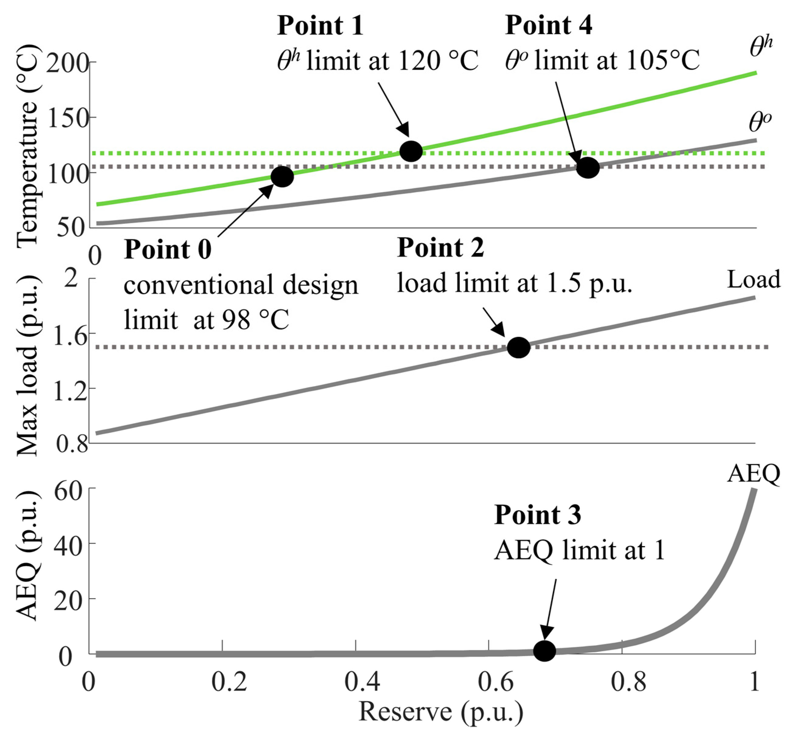
Figure 4.
Number of days where thermal limits are reached.
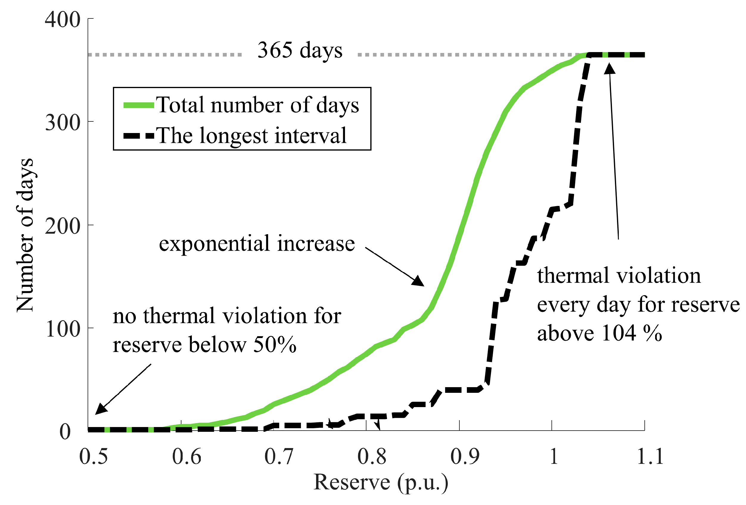
Figure 5.
The procedure for finding the needed Demand Response (DR) volume to interconnect the studied reserve.
Figure 5.
The procedure for finding the needed Demand Response (DR) volume to interconnect the studied reserve.

Figure 6.
Piece-wise linearization (PWL) process: (a) functions fitting and breakpoints; (b) mathematical formulation for function f1.
Figure 6.
Piece-wise linearization (PWL) process: (a) functions fitting and breakpoints; (b) mathematical formulation for function f1.
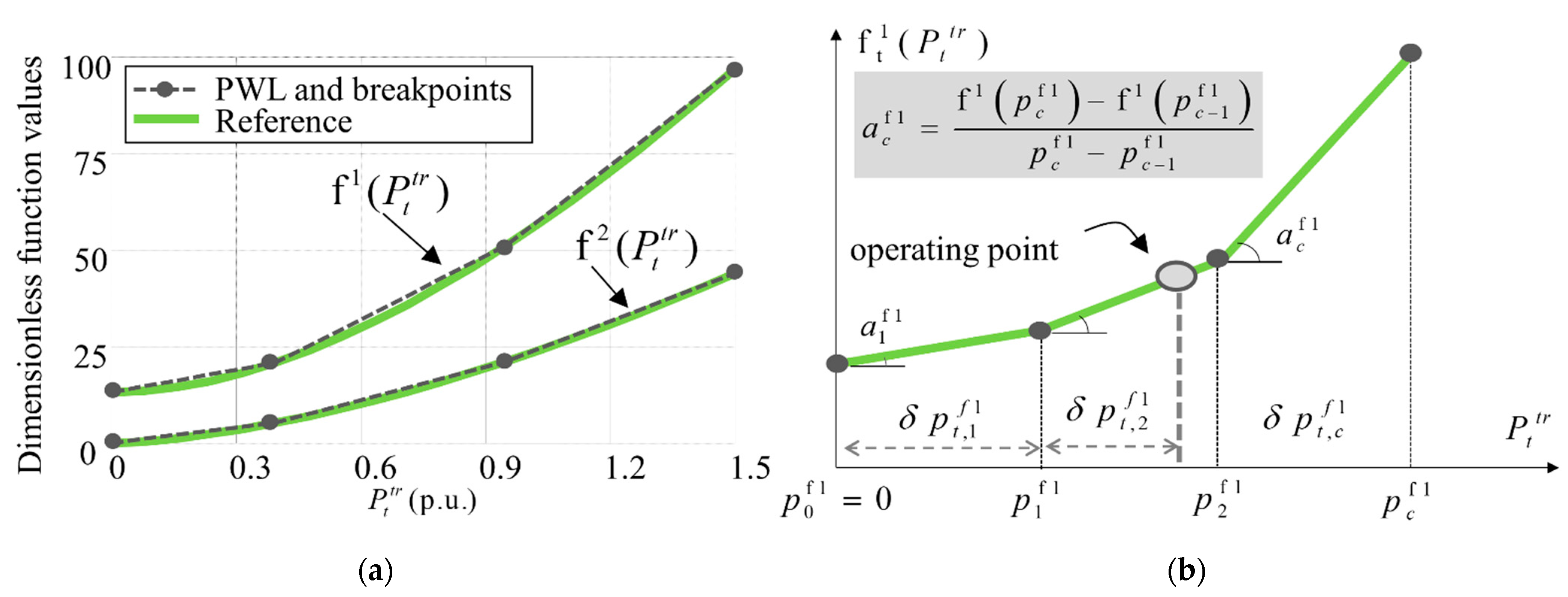
Figure 7.
PWL performances for different numbers of blocks—(a) top oil temperature; (b) hot spot temperature.
Figure 7.
PWL performances for different numbers of blocks—(a) top oil temperature; (b) hot spot temperature.

Figure 8.
PWL process: (a) functions fitting and breakpoints for fAEQ; (b) aging function—fAEQ error versus θh error.
Figure 8.
PWL process: (a) functions fitting and breakpoints for fAEQ; (b) aging function—fAEQ error versus θh error.
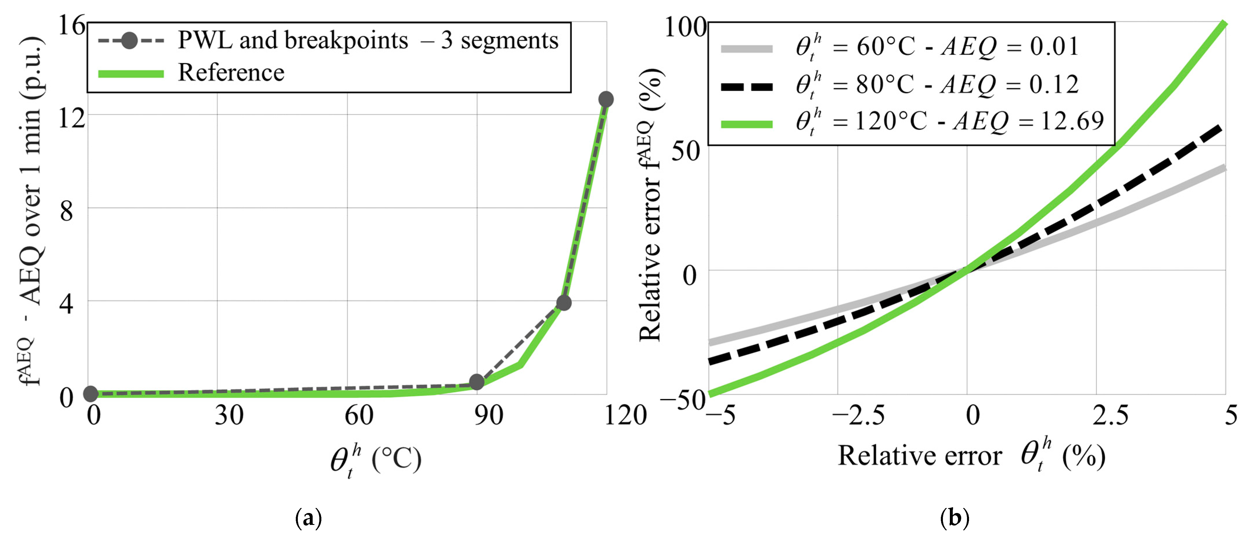
Figure 9.
Simulation with single and multiple time sets: (a) DR flexibility power; (b) transformer temperatures.
Figure 9.
Simulation with single and multiple time sets: (a) DR flexibility power; (b) transformer temperatures.
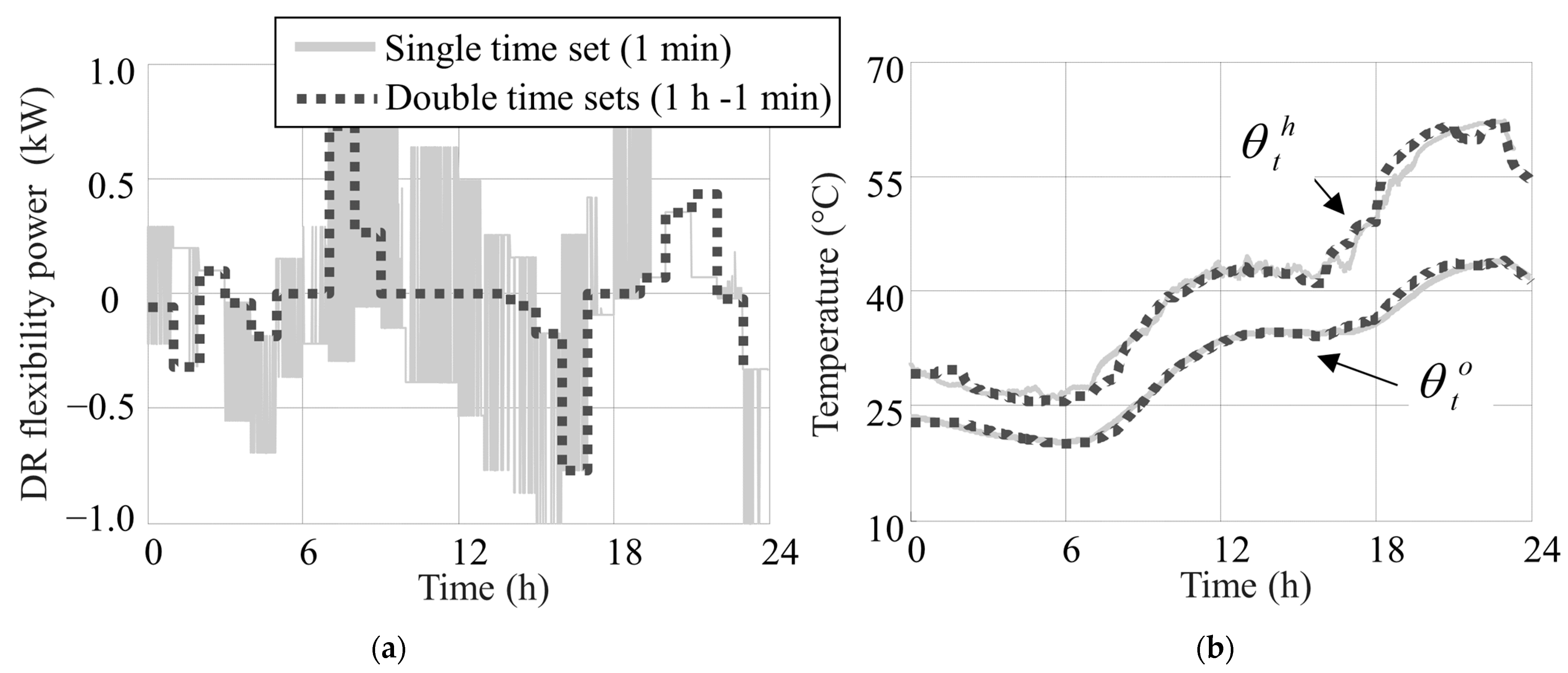
Figure 10.
Validation run with “energy shifting”: (a) transformer loadings; (b) temperatures.

Figure 11.
Validation run with “energy shedding”: (a) transformer loadings; (b) temperatures.

Figure 12.
Validation run with “energy shedding” and aging: (a) transformer loadings; (b) temperatures.
Figure 12.
Validation run with “energy shedding” and aging: (a) transformer loadings; (b) temperatures.

Figure 13.
One-week profiles in January, comparison of the base case and Dynamic Thermal Rating (DTR)/DR in “energy-shedding mode”: (a) transformer loading; (b) hot-spot temperature.
Figure 13.
One-week profiles in January, comparison of the base case and Dynamic Thermal Rating (DTR)/DR in “energy-shedding mode”: (a) transformer loading; (b) hot-spot temperature.

Figure 14.
Obtained results for different reserve margins and DR in “energy-shedding” mode: (a) DR rated power; (b) DR power share compared to the added load; (c) DR rated energy; (d) DR energy share compared to the total energy of load.
Figure 14.
Obtained results for different reserve margins and DR in “energy-shedding” mode: (a) DR rated power; (b) DR power share compared to the added load; (c) DR rated energy; (d) DR energy share compared to the total energy of load.
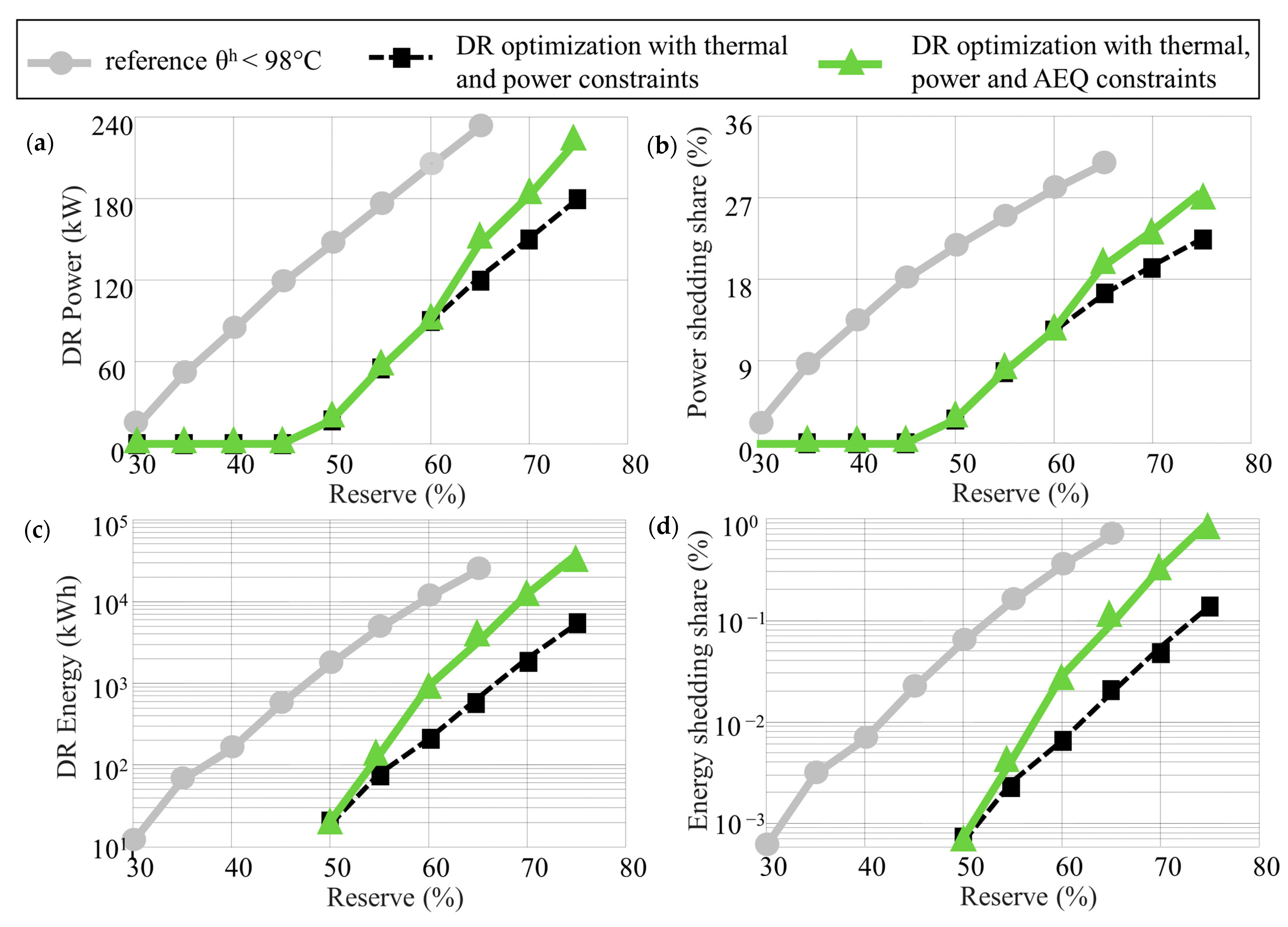
Figure 15.
Power shedding over the year—75% reserve in “energy-shedding” mode.

Figure 16.
Yearly temperature duration curves: 75% reserve in “energy-shedding” mode leading to less than 1% energy curtailment, as seen in Figure 14d.
Figure 16.
Yearly temperature duration curves: 75% reserve in “energy-shedding” mode leading to less than 1% energy curtailment, as seen in Figure 14d.
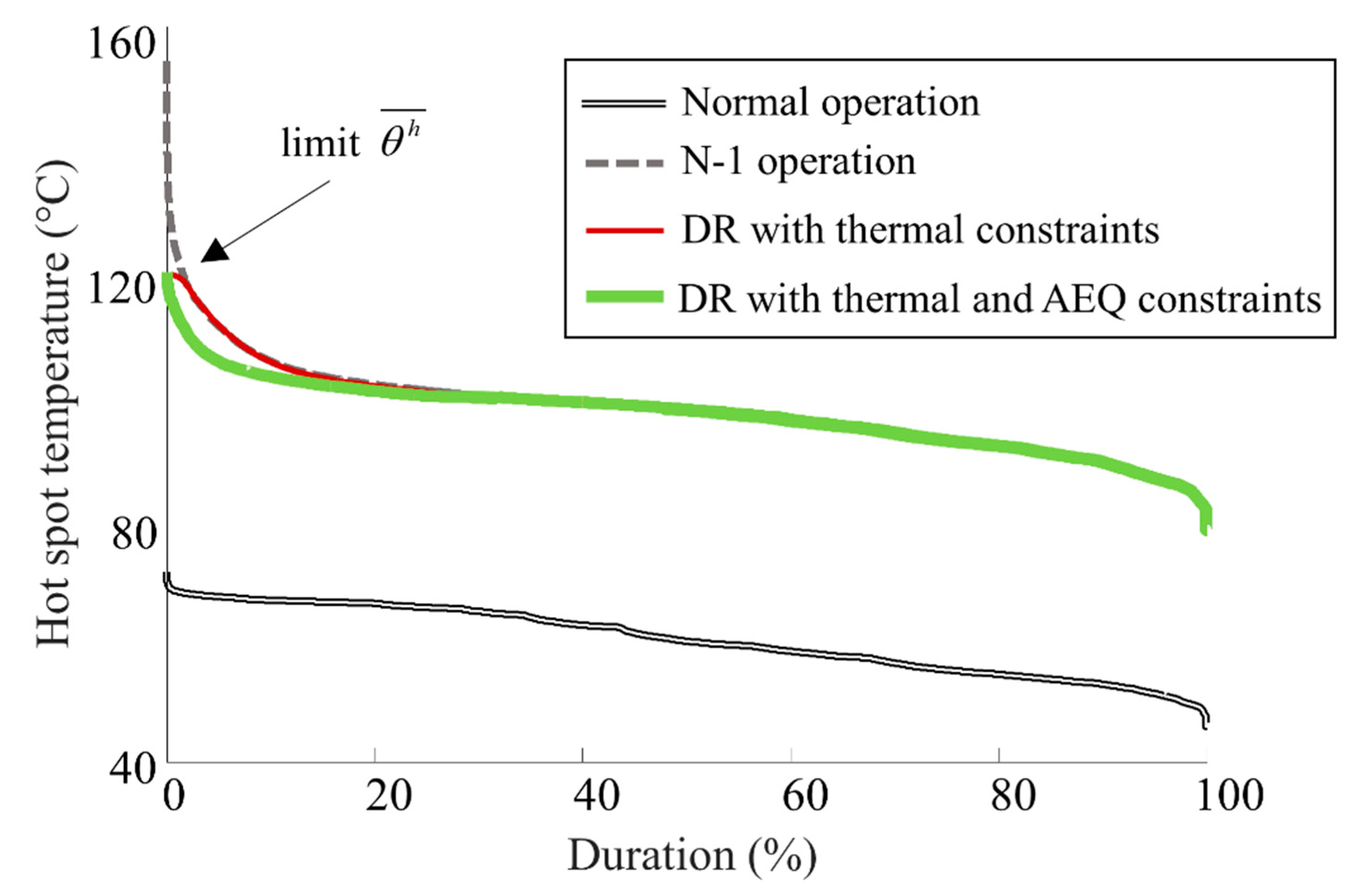
Figure 17.
Results: DR modeled with or without payback effect/energy conservation: (a) DR power in kW; (b) DR energy in kWh.
Figure 17.
Results: DR modeled with or without payback effect/energy conservation: (a) DR power in kW; (b) DR energy in kWh.

Figure 18.
Computation times for the nonlinear formulation (the blue line) and for the suggested PWL formulation (the green line). Both formulations were tested for the “energy-shedding” case ( = 100% and = 0%).
Figure 18.
Computation times for the nonlinear formulation (the blue line) and for the suggested PWL formulation (the green line). Both formulations were tested for the “energy-shedding” case ( = 100% and = 0%).


Table 1.
Limits for distribution transformers applicable for different types of loadings [42].
Table 1.
Limits for distribution transformers applicable for different types of loadings [42].
| Limits | Loading Type | ||
|---|---|---|---|
| Normal Cyclic | Long-Term Emergency | Short-Term Emergency | |
| Ptr (p.u.) | 1.5 | 1.8 | 2.0 |
| θh (°C) | 120 | 140 | Not specified |
| θo (°C) | 105 | 115 | Not specified |
| AEQ (p.u. | 1 | >1 possible | Not specified |
Table 2.
Thermal characteristics of ONAN (Oil Natural Air Natural) distribution transformers at nominal conditions.
Table 2.
Thermal characteristics of ONAN (Oil Natural Air Natural) distribution transformers at nominal conditions.
| x | y | R | τo | τw | θa |
| 0.8 | 1.6 | 5 | 180 | 4 | 20 |
| θh | Δθhr | Δθor | k11 | k21 | k22 |
| 98 | 23 | 55 | 1 | 1 | 2 |
Table 3.
List of the used symbols.
| Sets | Variables | ||
|---|---|---|---|
| DR flexibility power (kW) | |||
| Generic set of time step (1 min) | Transformer loading (p.u.) | ||
| Set of time step for dispatch (1 h) | , | PWL power in block c at t (p.u.) | |
| Set of PWL blocks | DR flexibility rated power (kW) | ||
| DR flexibility rated energy (kWh) | |||
| Transformer Parameters | |||
| Ambient temperature at time t (°C) | Oil/winding exponent | ||
| Top oil temperature at time t (°C) | Loss ratio, hot-spot factor | ||
| Hot-spot temperature at time t (°C) | Hot-spot factor | ||
| , | Hot-spot to top oil gradients at t (K) | Oil/winding time constant (min) | |
| Rated hot-spot to oil gradient (K) | , | Model coefficients | |
| Rated top oil temperature rise (K) | Transformer rated power (kW) | ||
| Simulation Parameters | |||
| Load to supply at time t (kW) | Lower/upper state of charge (%) | ||
| , | PWL breakpoints in block c | Initial flexibility state of charge (%) | |
| , | PWL slope in block c | Final flexibility state of charge (%) | |
Table 4.
Aging EQuivalent (AEQ) computation for different numbers of PWL segments.
| Number of PWL blocks for θo and θh | 6 | 6 | 6 | 6 | 9 | 12 |
| Number of PWL blocks for AEQ | 3 | 6 | 12 | 18 | 12 | 12 |
| AEQ computed with exact θo and θh | 0.67 | 0.88 | 0.94 | 0.94 | 0.95 | 0.96 |
| AEQ computed with PWL θo and θh | 0.70 | 0.91 | 0.97 | 0.97 | 0.97 | 0.97 |
| AEQ computed with PWL | 1.00 | 1.00 | 1.00 | 1.00 | 1.00 | 1.00 |
Publisher’s Note: MDPI stays neutral with regard to jurisdictional claims in published maps and institutional affiliations. |
© 2021 by the authors. Licensee MDPI, Basel, Switzerland. This article is an open access article distributed under the terms and conditions of the Creative Commons Attribution (CC BY) license (http://creativecommons.org/licenses/by/4.0/).
Share and Cite
MDPI and ACS Style
Daminov, I.; Rigo-Mariani, R.; Caire, R.; Prokhorov, A.; Alvarez-Hérault, M.-C. Demand Response Coupled with Dynamic Thermal Rating for Increased Transformer Reserve and Lifetime. Energies 2021, 14, 1378. https://doi.org/10.3390/en14051378
AMA Style
Daminov I, Rigo-Mariani R, Caire R, Prokhorov A, Alvarez-Hérault M-C. Demand Response Coupled with Dynamic Thermal Rating for Increased Transformer Reserve and Lifetime. Energies. 2021; 14(5):1378. https://doi.org/10.3390/en14051378
Chicago/Turabian StyleDaminov, Ildar, Rémy Rigo-Mariani, Raphael Caire, Anton Prokhorov, and Marie-Cécile Alvarez-Hérault. 2021. "Demand Response Coupled with Dynamic Thermal Rating for Increased Transformer Reserve and Lifetime" Energies 14, no. 5: 1378. https://doi.org/10.3390/en14051378
Note that from the first issue of 2016, this journal uses article numbers instead of page numbers. See further details here.