Assessing the Relation between Mud Components and Rheology for Loss Circulation Prevention Using Polymeric Gels: A Machine Learning Approach

Abstract

The traditional way to mitigate loss circulation in drilling operations is to use preventative and curative materials. However, it is difficult to quantify the amount of materials from every possible combination to produce customized rheological properties. In this study, machine learning (ML) is used to develop a framework to identify material composition for loss circulation applications based on the desired rheological characteristics. The relation between the rheological properties and the mud components for polyacrylamide/polyethyleneimine (PAM/PEI)-based mud is assessed experimentally. Four different ML algorithms were implemented to model the rheological data for various mud components at different concentrations and testing conditions. These four algorithms include (a) k-Nearest Neighbor, (b) Random Forest, (c) Gradient Boosting, and (d) AdaBoosting. The Gradient Boosting model showed the highest accuracy (91 and 74% for plastic and apparent viscosity, respectively), which can be further used for hydraulic calculations. Overall, the experimental study presented in this paper, together with the proposed ML-based framework, adds valuable information to the design of PAM/PEI-based mud. The ML models allowed a wide range of rheology assessments for various drilling fluid formulations with a mean accuracy of up to 91%. The case study has shown that with the appropriate combination of materials, reasonable rheological properties could be achieved to prevent loss circulation by managing the equivalent circulating density (ECD).

1. Introduction

Loss circulation is affected by many operational parameters, among the most important ones are the type of the mud base, rheological parameters, and mud weight. Other influential parameters can be attributed to the geomechanical properties such as in situ stresses, formation pore pressure, fracture gradients, and natural fractures (Salehi and Kiran, 2016). The design of drilling fluids and the selection of appropriate loss circulation materials (LCMs) are based on understanding the different types of loss zones and downhole conditions [1].

The strategy to manage loss circulation may vary on the severity of the loss. These strategies include two types of approaches: (a) corrective treatment and (b) preventive approach. The corrective treatment, which refers to any action taken after the occurrence of the losses, is often used to stop the loss and quickly regain mud circulation. The preventive treatment is a more reliable approach since it is a proactive treatment that aims to avoid the loss before entering the expected risk zone. The preventive approach has been validated by several experimental and field studies where substantial increases in fracture gradients, reduced number of casing string, and reduced non-productive time (NPT) were achieved through wellbore strengthening techniques [2].

In this endeavor, various LCM types such as polymers and crosslinked polymers are used [3,4]. Such materials are conducive to loss circulation prevention and viscosity enhancement for drilling fluid and cement [5,6]. Polymers can also help drill high-pressure/high-temperature (HP/HT) wells, where conventional water-based mud (WBM) regularly exhibits severe rheology deterioration. The WBM formulations can be significantly enhanced by using polymeric deflocculant to act as a rheology modifier and LCM.

Among many polymers used to enhance fluid-loss control and thermal stability, polyacrylamide (PAM) is the most favorable due to its exceptional rheological properties and low cost [7]. PAM forms viscoelastic fluids when crosslinked with a proper crosslinker. The crosslinking can be a chemical or a physical process that binds two or more molecular chains of monomer units to form the three-dimensional network of the crosslinked polymers [8].

Many crosslinkers have been widely used industrially for PAM crosslinking [9,10]. For example, organic crosslinkers have better durability and better gel control, particularly at elevated temperatures because the organic crosslinkers form covalent bonds and provide strong and thermally sfigure networks. One of the most abundantly used organic crosslinkers is polyethyleneimine (PEI) because of its wide temperature window and good gel control with retarders or accelerators [6,11].

1.1. Effect of Mud Composition on Rheology and Mud Hydraulics

In drilling operations, maintaining proper rheology is one of the main objectives of drilling fluid design. Rheology plays a fundamental role in drilling fluid efficiency and the ability to carry out its primary functions, such as cutting suspension and hole cleaning, carrying of mud solid, as well as creating sufficient hydrodynamic pressure inside the well [12,13]. The mud formulation and rheology also affect the fracturing of the rocks and absorption of drilling mud into rocks or fluid-rock interaction, in addition to mitigating formation damage [14,15]. Other mud functions include carrying out drilled cuttings to the surface, regulating hydrostatic pressure in the well to balance formation pressure, cooling and lubricating of the bit and drill string, plugging highly permeable formations, and stabilizing borehole.

Measurements of rheology are usually performed using equipment mostly standardized by the American Petroleum Institute (API) to quantify the relationship between the shear stress and shear rate. Mainly, the measurements are conducted at low-pressure and low-temperature conditions, which is not representative of downhole conditions. The high-pressure high-temperature (HPHT) measurements give a better determination of rheology. However, drilling fluids’ viscosity alternates due to contamination while drilling [16,17]. Currently, drilling bottom hole assemblies are equipped with downhole sensors for measurements while drilling (MWD). It can provide information on mud properties such as fluid density, viscosity, and flow rate [18]. Lie et al. (2013) conducted comprehensive laboratory experiments to validate data collected from downhole sensors in temperatures up to 347 °F. The experimental data showed a good correlation with the collected downhole measurements [19]. Still, there are some difficulties in getting real-time data due to the operational challenges and varying downhole conditions.

Table 1. Cons and pros for the used rheology determination approaches.

Approach	Pros	Cons
Laboratory experiments	Easy to conduct Parametric and screening study at the design stage Fundamental understanding of fluids flow characteristics	Difficulties in simulating reservoir parameters Difficult to account for drilling operational factors Downhole contaminations
Analytical modeling	Direct Relatively not expensive An extended range of estimation	Limited to assumptions and boundaries
Machine learning	Identifying trends and patterns Handling multi parameters More comprehensive applications and continuous improvement	Requires a relatively large amount of data Requires validation and careful parameter evaluation
Downhole measurement tools	Have high accuracy Consider fluid contaminations	Real-time measurement is a challenge Limited hole sizes Limited temperatures

summarizes the different approaches used in the oil and gas industry for rheology determination with their main pros and cons.

Therefore, the management of drilling fluid components and rheological characteristics of drilling fluid is a challenging process. Though, such problems can be solved in a well by chemical processing of drilling fluid by various polymers [20,21,22].

Moreover, for polymeric fluids, investigation of rheology is more important for better estimation of the gelation time and final gel strength [23,24]. A good estimate of the gelation time, which is the time taken by the crosslinking polymer to transform from fluid to gel, helps avoid gel formation in the piping system during the injection. Gelation is a function of many parameters, such as the polymer’s concentration and crosslinker, salinity, temperature, and resting time [25]. Additionally, proper mud formulation helps in the successful placement of the polymeric pill into the loss zone at the intended depth without the risk of gelling during the injection process. Therefore, in this paper, the rheology of polymer-based mud is investigated in interaction with different mud additives.

1.2. Data Science and Machine Learning Techniques

The use of large amounts of data for decision-making became practical in the 1980s; later, many studies described how different machine learning approaches can be applied to various industry problems [26,27]. Currently, the term “data science” is increasingly used in the industry. Data science implies using the knowledge extracted through systematic studies involving data analysis and its role in inference. The scalability in decision making that data science techniques have provided made it possible for the emerging of machine intelligence, fueled by data and state-of-the-art analytics. The machine learning approach surpasses the conventional statistical analysis in many ways; for example, analyzing heterogeneous and unstructured data requires defining the complex relationship between different entities, which is possible by machine learning [28].

In the quest for drilling data analysis, it is often difficult to accurately determine flow parameters during complex drilling operations, where the correct ECD calculation is crucial. Different fluid systems with various viscosity regimes are used at different stages of drilling. For instance, in the shallow sections of the well, less viscous fluids are used, such as water or brine, while more vicious clays can be added in the deeper sections [29,30]. Rheology characteristics of these different drilling fluids are usually evaluated by experimental studies and empirical correlations to determine viscosity behavior and stability as temperature changes [31].

Moreover, ECD management is possible with appropriate downhole pressure gauges and a good hydraulic model. Weikey et al. (2018) reviewed some of the techniques used to measure the rheology of drilling fluids [32]. However, the accuracy of such models also depends mostly on the quality of the rheology data [33]. Andaverde et al. (2019) developed a mathematical model for fluid flow analysis based on a nonlinear function that matches the measured data for shear stress and shear rate [34]. In a recent study, Skadsem et al. (2019) used the structural kinetics model proposed by Dullaert and Mewis [35] to model thixotropy and steady shear rheological measurements. Their model consisted of eight inputs of several different combinations of parameters and can produce predictions that fit the experimental data [36]. Kiran and Salehi (2020) proposed machine learning (ML)-based classification to identify the lost circulation zone based on drilling parameters in advance [37]. The use of such frameworks, combined with the predictive ability of ML, can be used to develop a preventive strategy for efficient drilling operations. The ML application in drilling fluids design is fairly new, and the goal here is to investigate ML techniques for crosslinked polymeric mud comprising PAM and PEI.

2. Methodology

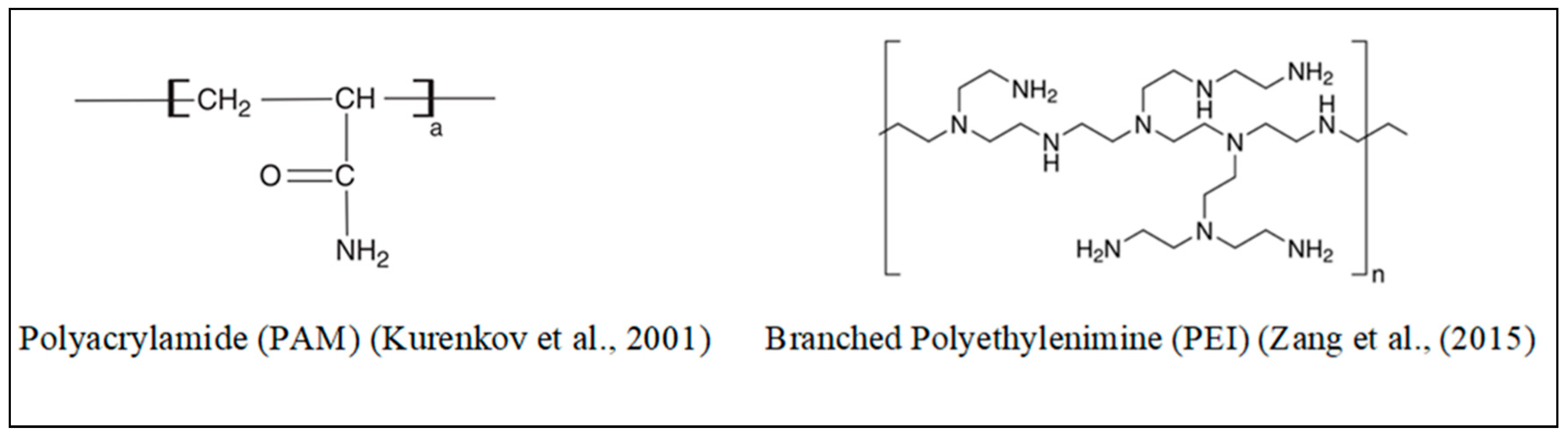
2.1. Materials

Several chemicals are used to enhance or customize the drilling fluid properties. One of the materials used as a drilling additive to mitigate lost circulation is polyacrylamide (PAM). PAMs are water-soluble polymers produced by polymerization of the acrylamide monomer. In this study, unlike the common treatment, PAM is used as the main viscosity additive, which at a proper concentration should provide sufficient rheological parameters for drilling fluids. A commercial PAM consisting of acrylamide monomers was obtained from SNF Floerger Group, France. The active matter of the received material was 20 wt.%, dissolved in distilled water. PAM has a relatively low molecular weight (Mw) of about 200,000 Da and therefore provides moderate viscosity of about 70 mPa.s for a concentration of 7%.

PAM forms viscoelastic fluid when crosslinked with a proper crosslinker. The crosslinkers can enhance the gel strength of the drilling fluid and form a strong mature gel at the designed activation condition and subsequently serve as sealing materials for fractured formations. The gel strength is required for the suspension of solids and weighting material when circulation is stopped. In this study, an organic polymer, polyethyleneimine (PEI), was used as a crosslinker. One of the major advantages of using such an organic compound lies with its environmental compatibility. The crosslinker was a highly branched PEI with Mw of 750,000 Da and a concentration of 33.3 wt.%. The chemical structures of PAM and branched PEI are shown in Figure 1.

In addition to the two above-mentioned fluids, other essential drilling fluid additives including barite as weighting agent, caustic soda to raise the pH of the mud and clay dispersion, and lignite as mud dispersant were used. Cedar fiber was also integrated with the crosslinked polymer as an example of the conventional LCM used in the normal drilling operation. All materials from commercial suppliers were used as received. The experimental matrix was designed to investigate the dependency of the rheological properties on each component of the drilling fluid formula. The three major contributors to the rheology are the amount of PAM, PEI, and bentonite. Therefore, these three components were varied from the minimum to the maximum amount expected to result in reasonable viscosities for drilling fluid application. The effect of other drilling fluid additives was incorporated using an appropriate range of concentrations for each additive. Each parameter was varied separately, keeping others constant at their optimum values, and each formula was tested at four temperatures. This experimental matrix formed the rheological properties dataset for a wide range of different component combinations under the selected temperature conditions. Machine learning algorithms were then used to evaluate the relationship and the rheology dependency for any fluid design based on this established interrelationship. The selected concentrations are described in

Table 2. Mud component and their range of concentrations.

Component/Temperature	Concentrations								lb/bbl	Weight %
PAM (lb/bbl)	5	6	7	7.5	8	9	10	12.5	17–44	5–12.5
PEI wt.% (lb/bbl)	0	0.25	0.5	0.8	1	1.25	1.5		0.8–5	0.25–1.5
Bentonite wt.% (lb/bbl)	1	2	2.5	3	3.5	4	5		0–5	0–1.5
Caustic soda (lb/bbl)	0	0.5	1	1.5					0–1.5	0–0.4
Mud weight (ppg)/ Barite (lb/bbl)	9.5/ 10	10/ 54	11.5/ 90						10–90	2 to 30
Fiber (lb/bbl)	0	5	10						0–15	3.5
Temperature (°F)	70	120	160	200

.

2.2. Rheology Measurements

An automated API certified speed dial viscometer was used for the rheological characterization. The samples of drilling fluids were prepared in a specific mixing order, as they appear in Table 2, to ensure good dispersion of additives and stability in the mixture with the polymer and the crosslinker. The samples were prepared using different combinations of additives with different concentrations, and the rheological measurements were obtained for each at four different temperatures, 75, 120, 160, and 200 °F. The samples were heated at 4 °F/min while stirring at 100 rpm to ramp up to the desired temperature. After reaching the desired temperature, the measurements were taken at various shear rates from 5.1 to 1021 s^−1, equivalent to 3 to 600 rpm. Using these measurements, the apparent viscosity, plastic viscosity, and yield point were calculated. These rheological properties are the most important design factors for drilling fluids. The AV is the fluid viscosity measured at a specific shear rate. According to API, the AV is defined for the Bingham plastic rheology model as one-half of the dial reading at 600 rpm, which gives a shear rate of 1022 s⁻¹. The PV, on the other hand, represents the viscosity of the fluid corresponding to an infinite shear rate. PV is the slope of the shear stress versus shear rate based on the Bingham plastic rheology model. The PV is calculated from the difference between the dial reading at 600 and 300 rpm. YP is expressed in pounds per 100 ft² and calculated by subtracting plastic viscosity value from the dial reading at 300 rpm.

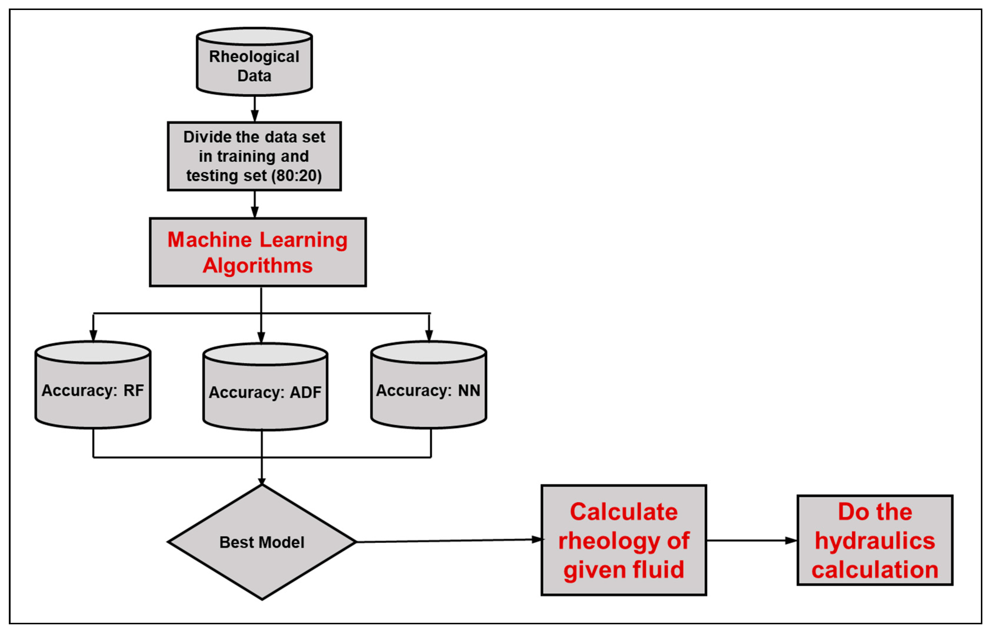
2.3. Data Analysis

With the rheological measurements, a workflow is constructed to automate the process of identifying suitable drilling fluid for field applications. The suitability of the drilling fluid depends on the compatibility and workability, based on its rheological properties. After deciding the desired rheological properties, the material required to achieve these rheological properties can be obtained using the machine learning programs. To build the ML modules, the experimental data and rheological properties are used for training and testing. The broader framework is illustrated in Figure 2. The experimental data are used as input, which consist of the amount of materials, temperature, and the rheological properties such as plastic viscosity, apparent viscosity, and yield point. The dataset consisting of 284 data points was randomly split in 80:20 to train and test different algorithms. The machine learning algorithms used in this study were (a) k-Nearest Neighbor, (b) Random Forest, (b) Gradient Boosting, and (d) AdaBoosting. The details of the algorithms are presented in the next section. These algorithms were run 50 times to identify the deviation in the results by repetitively running the algorithms and comparing the standard deviations.

3. Machine Learning Algorithms

Various recipes of drilling fluids were prepared by using different combinations of the selected additives. Different combinations of components were set at the ranges described in Table 2. They were tested under each of the four targeted temperatures to generate 71 data sets consisting of 284 data points.

In the world of data science, machine learning is a highly sought technology to implement in real-time operation. Machine learning algorithms have been constantly used from operational optimization to fraud detection, from identifying the compressor’s problem to predicting the customer’s choice. The ever-increasing implementations of these algorithms are also widely used for the predictive purpose embedded in the datasets. A word of caution must be described before proceeding further with the implementation of such algorithms. The downhole operational datasets in oil and gas are different from the workable day-to-day dataset (health data, financial data, customer preferences, etc.), where the implementation has been highly successful. Hence, it becomes natural to test different algorithms. Here, we have used four regression supervised learning algorithms to train and test the regression models for the experimental rheological data. The following section describes the regression models implemented in this study, which are (i) K-Nearest Neighbor, (ii) Random Forest, (iii) Gradient Boosting, and (iv) AdaBoosting.

3.1. k-Nearest Neighbor (kNN) Algorithm

One of the most popular regression models is based on the k-Nearest Neighbor (kNN) algorithm. This algorithm can be used in combination with other mathematical rules to test the predictive capability. Modaresi et al. (2017) used kNN to evaluate the monthly inflow of the Karkheh dam [38]. Other authors [39] proposed a kNN regression model for geo-imputation for pattern-label-based short-term wind prediction of spatial–temporal wind data. Similarly, [40] used it to map a demonstrated grasp motion by a human hand to a robotic hand. Apart from other industries, the petroleum industry is frequently implementing these algorithms for prediction purposes. One study [41] compared different machine learning algorithms, including kNN, to predict reservoir fluid properties. The success of this regression model is highly dependent on the distance metrics from the nearest neighbors. One of the most commonly used metrics is Euclidean distance [42]. The algorithm uses the number of the nearest neighbors of the test instance for the label sets of its neighboring instances. After identifying the desired nearest neighbors, the predictive value for input data is the mean output of the identified samples. The algorithm is considered slow due to its inbuilt nature of scanning the whole data set for each prediction [43].

3.2. Random Forest Regression

The Random Forest (RF) algorithm is a robust supervised machine learning algorithm, which is a combination of decision trees. A decision tree algorithm can produce erroneous results due to variance and overfitting in the predictions. Hence, to overcome this anomaly, a set of decision trees is framed, and the average values of all decision trees are used to produce the final result [44]. This RF regression model improves individual estimator performance by adopting an ensemble-based combined performance strategy [45,46]. It has been implemented in a range of predictive modeling, including object recognition, chemoinformatic, bioinformatics, and air quality prediction [47,48,49]. In the oil and gas industry, RF has also gained traction over time. Hedge et al. [50] used Random Forests to predict the rate of penetration during drilling.

Breiman (2001) constructed a set of decision trees based on nonparametric regression estimation for Random Forest modeling. A predictor is implemented, which consists of a collection of randomized regression trees. The predictor estimate for the regression is defined by the following function [51]:

$$m_{M,n}\left(\mathit{X};{\theta }_1,{\theta }_2\dots .,{\theta }_M,D_n\right)=\frac{1}{M}{\displaystyle \sum }_{j=1}^M{\displaystyle \sum }_{i\in D_n^{*}\left({\theta }_j\right)}\frac{1_{X_i\in A_n\left(x;{\theta }_j,D_n\right)}{Y}_i}{N_n\left(\mathit{X};{\theta }_j,D_n\right)}$$

(1)

Equation (1) gives the predicted values for the number of trees (j^th) at the query point x. The prediction uses the independent random variables of the training sample expressed as $D_n$, which is associated with the variable number (n). The predicted value at (x) is denoted by $m_{M,n}\left(\mathit{X};{\theta }_1,{\theta }_2\dots .,{\theta }_M,D_n\right)$ where θ₁, θ₂, …, θ_M are independent random variables for each query point (x) located at m and n order. These are randomly distributed and independent of the training sample variable ($D_n$). $A_n$ represents the set of data points selected before tree construction and expressed in the form of a matrix where $A_n\left(x;{\theta }_j,D_n\right)$ denotes the cell containing the query point x. The number ($N_n$) of the cell that falls into the query point is expressed by the term $N_n\left(\mathit{X};{\theta }_j,D_n\right)$. Equation (1) also uses the output data point ($Y_i$) related to the query point (${ }_i$) to generate the predictions.

The error in RF predictions depends on the correlation between any two nodes in the forest and individual nodes’ strength. The higher correlation between nodes leads to a higher error rate, while greater strength reflects the reduction in error, which is affected by the size of the subset of the variables used in tree building. The central theme of RF is to improve the reduction in the variance of bagging by reducing the correlation between the nodes without a substantial increase in the variance. This can be achieved by growing the nodes through a random selection of the input variables [51]. The decision tree can be expanded to its maximum depth using a combination of features from the input parameters. RF also helps rank the features conducive to prediction estimates; however, we have only seven different input parameters. Therefore, we have solely focused on testing the accuracy of the test dataset.

3.3. Gradient Boosting Regression

Gradient Boosting (GB) is another type of ensemble supervised machine learning program which utilizes an additive model in a forward stage-wise fashion [52]. Like the Random Forest, it also uses decision trees as a basic building block for an ensemble of weak models [53]. It uses an individual weak complementary regressor sequentially, where a new weak learner is constructed to provide maximum correlation with the negative gradient of loss functions at each stage of iterations [54]. After these loss functions are implemented, a strategy similar to the artificial neural network is adopted. One of GB’s common loss functions is logistic regression, which is implemented in this case [55,56]. A decision tree is then used to make a prediction based on a series of rules that consist of different nodes. The difference between prediction and actual values depicts the error rate. This error rate is represented in the form of a gradient, which is the partial derivative of the loss function. The gradient is used to minimize the error for the next round of training. The extreme Gradient Boosting speeds up tree construction and uses a new algorithm for tree searching [57].

3.4. AdaBoosting Regression

The AdaBoost algorithm, inspired by numerical optimization and statistical estimation, uses a sequence of a simple weighted weak base classifier to construct a strong classifier. In each step, it attempts to find the optimal estimator as per weight distribution. Each estimator’s performance defines its weight in the next iteration, and finally, accurate predictors get more weightage eventually [58,59]. Friedman et al. (2000) used this concept and implemented statistical concepts for stagewise additive logistic regression to minimize the exponential loss function in additive boosting [60]. Lebanon and Lafferty (2002) studied the difference between AdaBoost’s approach and the maximum likelihood approach relying on the normalization to form a conditional probability over labels by the latter [61]. Madhuri et al. (2019) implemented the algorithm to estimate house prices and compared it with other regression techniques [62].

4. Results and Discussion

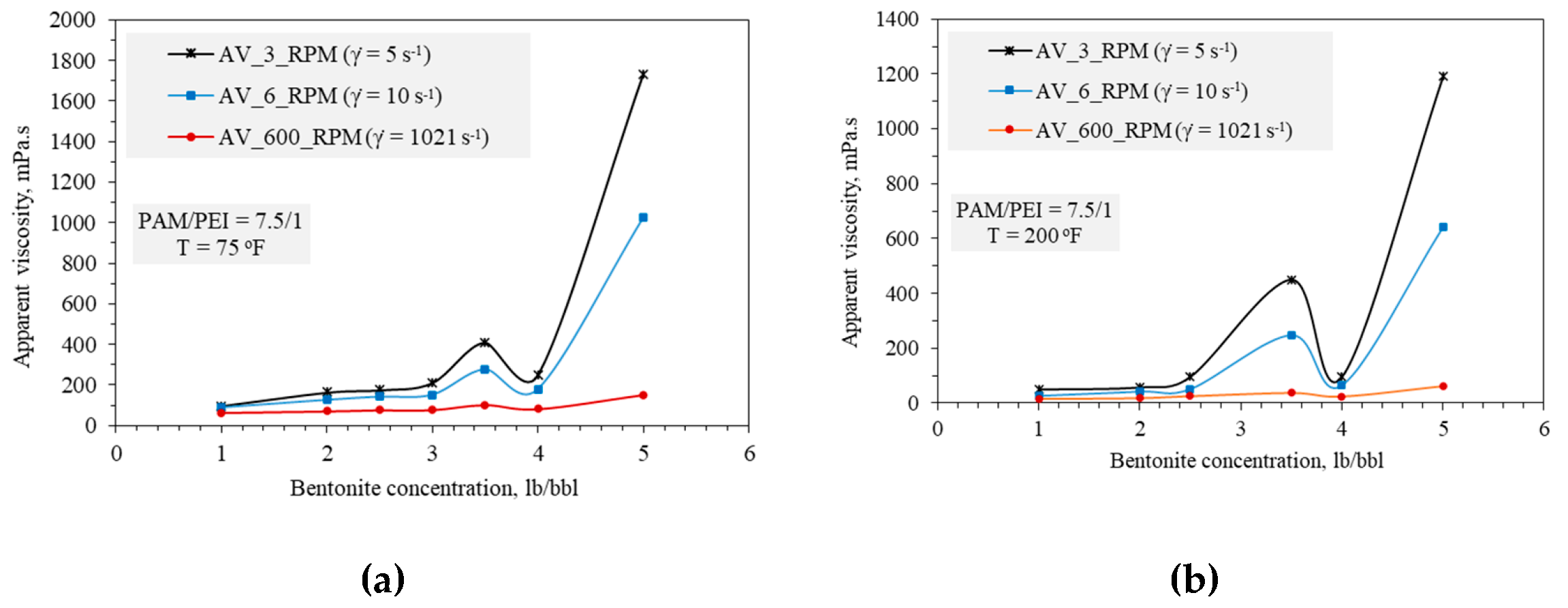
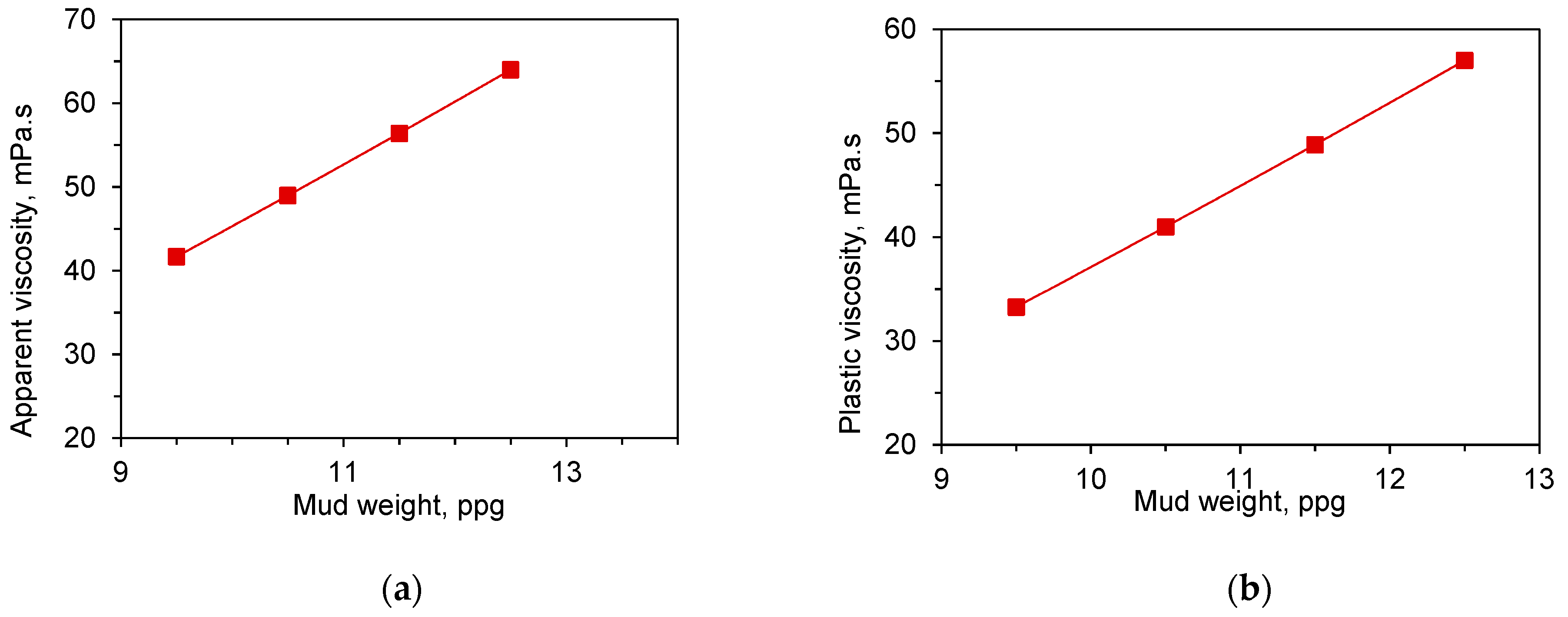
4.1. Rheology Data

The rheological data were generated based on the different mud recipes, amount of materials, and sample temperature. In this section, the impact of PAM, bentonite, and mud weight on the rheological properties (such as plastic viscosity, apparent viscosity) is highlighted. Different PAM concentrations of 5 to 12 wt.% were considered to determine the effect of the polymer concentration on the hydraulics of the drilling fluids and thus the equivalent circulation density (ECD). Figure 3 shows the PV calculated from the viscometer measurements of the different PAM concentrations prepared from non-crosslinked PAM in distilled water. The AV values at shear rates of 1021, 10, and 5 s⁻¹ for different PAM concentrations are shown in Figure 4. The values presented also show the effect of temperature, which was more pronounced in the low shear rates.

Both AV and PV were found to be exponentially increased with PAM concentration. Rational values were obtained with polymer concentrations of 7.5 to 10 wt.%. Beyond these PAM concentrations, the viscosities tended to increase drastically. Polymer tends to exhibit high viscosities at this high concentration of 10 to 12.5 wt.%; however, at elevated temperature (200 °F), a 70 to 75% reduction in viscosity was observed compared to the values measured at surface temperature.

Moreover, as the main viscosity additive in the water-based drilling fluids, bentonite was given a special focus in this study. The interaction between bentonite and PAM/PEI system was investigated. A significant improvement in rheology with bentonite addition was observed. Since PAM fluid’s viscosity deteriorates as temperature increases, bentonite enhanced the thermal stability of the PAM/PEI-based drilling fluid. Figure 5a,b shows the enhancement on the 7.5/1 wt.% PAM/PEI fluid with bentonite addition in amounts of 1 to 5 lb/bbl, which is 0.25 to 1.24 wt.% of the mud recipe. The improvement in viscosity was more pronounced under the high shear rates, especially at elevated temperatures (200 °F). There was a noticeable improvement in the PAM/PEI solutions’ viscosity with bentonite addition; the viscosity increased by approximately 170%. For example, PAM’s viscosity at 200 °F was tripled by adding 5 lb/bbl of bentonite. Similar behavior was observed at low shear rate (10 and 5 s⁻¹). It is worth mentioning that rheology of PAM/PEI with bentonite depends on the mixing procedures; a stable suspension and high viscosity is observed when bentonite is dispersed first in water before adding the crosslinked PAM/PEI polymer. The value of 3.5 lb/bbl of bentonite yielded a local maximum at all shear rates.

Finally, after the mud recipe was prepared, the proper mud weight was obtained by adding barite to the PAM/PEI based fluid. The nature of polyacrylamide interaction with barite was investigated by rheological measurement and physical observation of the PAM/PEI-based mud’s stability after barite addition. Barite sagging was lower at higher PAM concentrations, given the fact that viscosity increased with PAM concentration, as shown above. Moreover, Figure 6 shows that the interaction of barite particles with the PAM/PEI system had a positive impact on viscosity. The AV of a 7.5 wt.% PAM/PEI increased by 50% when mud weight increased from 9.5 to 11.5 ppg, and so did the PV. This fact can be used to optimize the PAM concentration to match the targeted mud weight dictated by the drilling program design. In some situations, conventual LCM such as fiber may be used in the WBM formulations, which will alter the viscosity of the fluid. Figure 7 shows the effect of cedar fiber in concentrations from 0 to 10 lb/bbl. Generally, fiber increased the viscosity of the mud and increased its thermal stability due to the gelation effect at elevated temperatures. This phenomenon was clearly visible by the less decay in viscosity versus temperature profile with fiber shown in Figure 7.

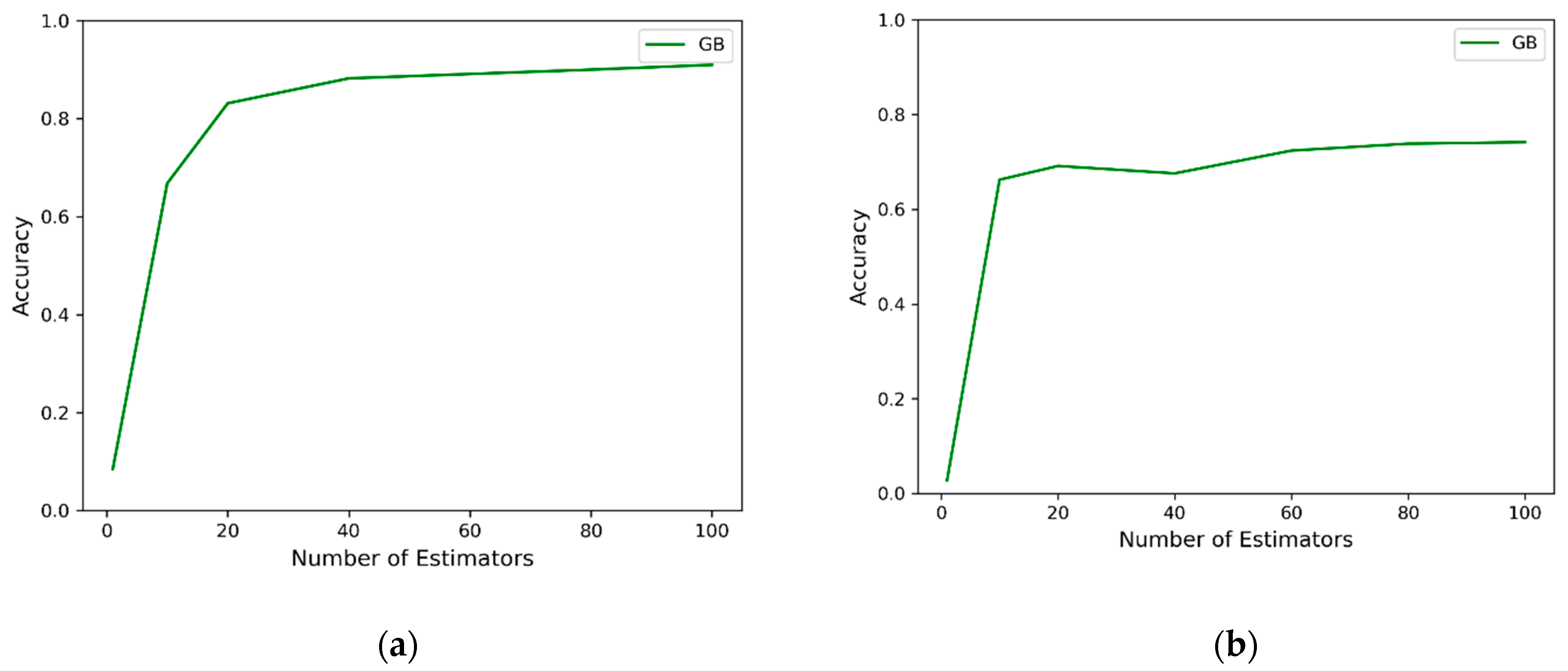
4.2. Tuning of Models Parameters

This section explains the tuning of parameters to obtain the highest accuracy by each algorithm. First, a simple kNN algorithm was implemented to train the data set based on input parameters consisting of the amount of different materials and operating temperature and output parameters as plastic viscosity and apparent viscosity. The main tuning parameters used in the kNN algorithm included weight, algorithm, leaf size, power parameter, and metrics. A uniform weight was applied, and the algorithm implemented was auto, which decides the most appropriate algorithm (BallTree and KDTree) based on values passed to fit methods. The leaf size and power parameter used in this study were 30 and 2, respectively. Standard Euclidean distance metrics were implemented. The maximum accuracy for predicting plastic and apparent viscosity was 77.9% and 67.8%, respectively.

As described earlier, the kNN algorithm’s accuracy depends on the number of nearest neighbors. We varied the number of nearest neighbors to get an insight into the behavior of the algorithm. A significant change in the predictive accuracy of the data set was observed with the change in the nearest neighbors, as shown in Figure 8. The maximum accuracy was found to be in the case of 3 closest neighbors sampling for plastic and apparent viscosity.

For the RF, the mean square error was used to measure the quality of split and variant reduction. The nodes were chosen to expand until all leaves contained less than two samples or all leaves were pure. The minimum number of samples for establishing the leaf node and weight fraction of the sum total of weights was considered to be 1 and 0, respectively. This machine learning model is based on different materials; hence, each parameter will be necessary to identify the rheological properties. Therefore, all six parameters were used as features in the model. Other tuning parameters included a relative reduction in impurity by specifying maximum leaf nodes, minimum impurity decrease and split, bootstrap, out-of-bag samples, random state, verbose, warm start, minimum cost-complexity pruning, and maximum samples, which were set to the default value. The main tuning parameter was the number of trees, which varied from 0 to 100. Figure 9 shows the accuracy of the prediction for plastic viscosity and apparent viscosity. In this study, the accuracy increased with increasing the number of trees up to 20. After 22 trees for PV and 13 trees for AV, it became asymptotic, as depicted in Figure 4a,b. The maximum accuracies for RF prediction for plastic viscosity and apparent viscosity were 87.9% and 60.6%, respectively.

Moreover, for the GB the least-squares regression was used for the optimization of the loss function. The learning rate for shrinkage contribution from each tree was considered to be 0.1. Additionally, the measurement of the quality of a split was estimated by the mean-squared error with an improvement score by Friedman. Other tuning parameters were incorporated as default. The main attribution used for testing the performance of the model was the number of boosting stages. Past studies suggest that the number of boosting stages directly impact the performance of the model. Hence, the number of boosting stages and the accuracy of the test data for plastic viscosity and apparent viscosity are plotted, as shown in Figure 5. The accuracy increased with an increase in the boosting stages as shown in Figure 10, and it reached a steady-state in the vicinity of 20 iterations. The maximum from this algorithm for plastic viscosity and apparent viscosity was found to be 90.7 and 74.3%, respectively.

Finally, for the AdaBoost algorithm, the main tuning parameters implemented in this study were base estimator, number of estimators, learning rate, loss, and random state. The base estimator and learning rate considered were 3 and 1, respectively. The number of estimators was varied in the form of boosting stages. The AdaBoost algorithm’s performance depends on the iterative steps, which improves estimators’ performance with the boosting stage. In this study, the algorithm was tested corresponding to the increase in the boosting stage. Results suggest that the maximum accuracy was achieved in the vicinity of 25 boosting stages, as shown in Figure 11. The maximum accuracy was 88.5% and 74.3% for plastic viscosity and apparent viscosity, respectively, as shown in Figure 6.

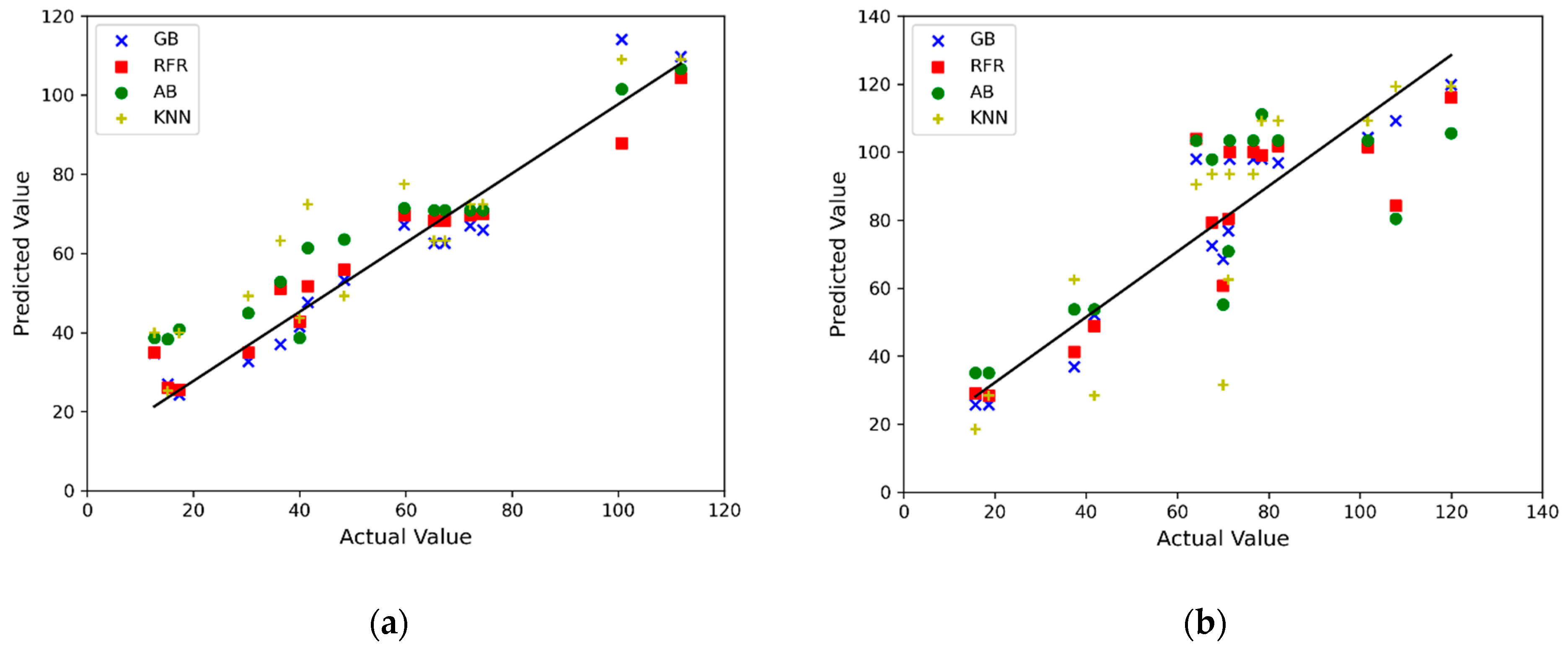
4.3. Performance and Accuracy of Predictions

By using different algorithms, valuable predictions of rheological data can be obtained for other systems of PAM/PEI and mud additives. Figure 12 compares the predicted values of the testing data set with actual values using the four algorithms tested in this study for the high shear rate values. It can be inferred that the overall predictive capability of Gradient Boosting was higher than any other algorithm for plastic and apparent viscosity. However, AdaBoost’s performance in predicting a higher range of plastic and apparent viscosity trumped other algorithm performances. Applying the same methodology for the low shear rate data was challenging. The prediction performance reduced significantly, and the predicted values differed from the actual values as shown in Figure 13. In pursuit of assessing these algorithms’ efficiency, the dataset was randomly selected for training and testing in a 20:80 ratio. For both viscosity values, each algorithm was executed 20 times, and statistical analysis was conducted.

Table 3. Performance of algorithms in predicting plastic and apparent viscosity (R²).

Algorithms	Performance
	Plastic Viscosity	Apparent Viscosity
k-Nearest Neighbor	0.69	0.48
Random Forest	0.88	0.60
Gradient Boosting	0.89	0.74
AdaBoosting	0.75	0.37

shows the overall result for each algorithm for the high shear rate data.

It is evident from the type of input parameters of rheological data that the data set was imbalanced. Several researchers have concluded that the Gradient Boosting performs better than other algorithms for imbalanced datasets (Brown and Mues, 2012; Ma et al., 2017). Overall, it can be observed from the results compiled in Table 2 that the performance of Gradient Boosting was better than other algorithms. Furthermore, it is worth mentioning that increasing the size of the dataset increases the algorithms’ predictive capabilities.

In conclusion, with the proper amount of materials, PAM/PEI-based mud can be designed to give the required rheological properties. PAM/BEI-based mud can work efficiently in replacing water-based mud when loss circulation occurs. The gelation characteristic of the crosslinked PAM/PEI mud will help to cure the loss circulation once the mature gel develops in the formation after the fluid invades the loss zone, as shown in our previous work [24]. However, one of the main challenges facing the drilling process is managing the overbalance between the ECD and formation pressure, especially in wells with a narrow window between the fracture gradient and the pore pressure gradient. The tool we are developing here allows for recipe manipulation to come up with the proper combinations of materials to provide the appropriate rheological properties that can have a better impact on the ECD.

A case study was used to validate this finding. A well with the information provided in

Table 4. Mud and well information used for the hydraulic calculations.

Component		Parameter	Information
Mud information	Mud Density	9.5	ppg
	Water-based mud	AV = 32, PV = 22	mPa.s
	PAM/PEI-based mud	AV = 27, PV = 26	mPa.s
Well information	Well Depth	6000	Ft
	Surface Hole Diameter	9 5/8	In
	Main Hole Diameter	7 7/8	In
	Casing Depth	3500	Ft
Drill Collar Information	ID	2 1/4	In
	OD	6 1/4	In
	Total Length	270	Ft
Drill Pipe Information
	ID	3 5/6	In
	OD	4.5	In
	Total Length	6430	Ft
Flow Rate Information	Pump rate	275	gpm
	Surface Pressure loss	100	Psi

was drilled to 6000 ft using water-based mud. Figure 14 shows the ECD calculated using water-based mud and PAM/PEI-based mud. From the results, it is clear that the same well can be drilled using the PAM/PEI-based mud of 9.5 ppg. Moreover, the circulating pressure obtained by the PAM/PEI-based mud was less than the one obtained by the WBM. The crosslinked polymer-based mud used to calculate the ECD consisted of 7.5 wt.% PAM and 1% PEI.

Table 5. Composition of the PAM/PEI-based mud and the water-based mud.

Component	PAM/PEI-Based Mud lb/bbl	Water-Based Mud lb/bbl
Water	312.3	318
Caustic soda	0.5	0.5
Lignite	0	4
Bentonite	3.5	20
Mud deflocculant	0	4
Calcium Carbonate	0	55
PAM	25.6	0
PEI	3.4	0
Barite	56.3	0.85

shows the full component and composition of the two mud systems.

5. Conclusions

The lack of a comprehensive predictive model for the rheological properties of crosslinked polyacrylamide-based drilling fluid was the primary motivation behind this study. Moreover, the nature of the interaction of PAM/PEI and the drilling fluid additives is not fully understood. Therefore, a holistic experimental and computational solution was developed to predict the rheological properties, which can address the loss circulation problem at a certain depth and temperature.

First of all, the rheological data were collected in the experimental environment for PEI/PAM-based drilling fluid. The experimental study quantified the appropriate amount of PAM/PEI with other additives for reasonable and competent rheological properties conducive to better ECD. Additionally, the experimental data were used in machine learning algorithms to assess the best-suited model for rheological characterization. The machine learning algorithms included regression-based models using k-Nearest Neighbor, Random Forest, Gradient Boosting, and AdaBoosting algorithms. These models allowed a wide range of rheology evaluation for different drilling fluid compositions comprising PAM crosslinked with PEI. Overall, the following conclusions can be drawn from this study:

(a)

Rheology of PAM/PEI-based mud is highly dependent on the PAM concentration rather than PEI concentration. Best values ranged from 7 to 10 wt.%. Other materials had less impact on viscosity; however, the PAM concentration should be optimized accordingly to achieve targeted rheology, especially for the high solid contents such as barite.

(b)

In the case of an imbalanced dataset of rheological characterization, Gradient Boosting performed significantly better than other algorithms, including k-Nearest Neighbor, Random Forest, and AdaBoosting.

(c)

The accuracy from the Gradient Boosting algorithm was 91 and 74% for plastic viscosity (PV) and apparent viscosity (AV), respectively. This algorithm’s maximum accuracy was obtained to be 91 and 74% for PV and AV, respectively. It is worth noting that this variation can be minimized using a greater number of data-points.

(d)

The rheology data at the low shear rate were challenging, although the performance of prediction was very low; still, some good predictions were obtained at the low values of viscosities where low concentrations of mud additives were used. Increasing the size of the data set is expected to increase the performance of the model.

(e)

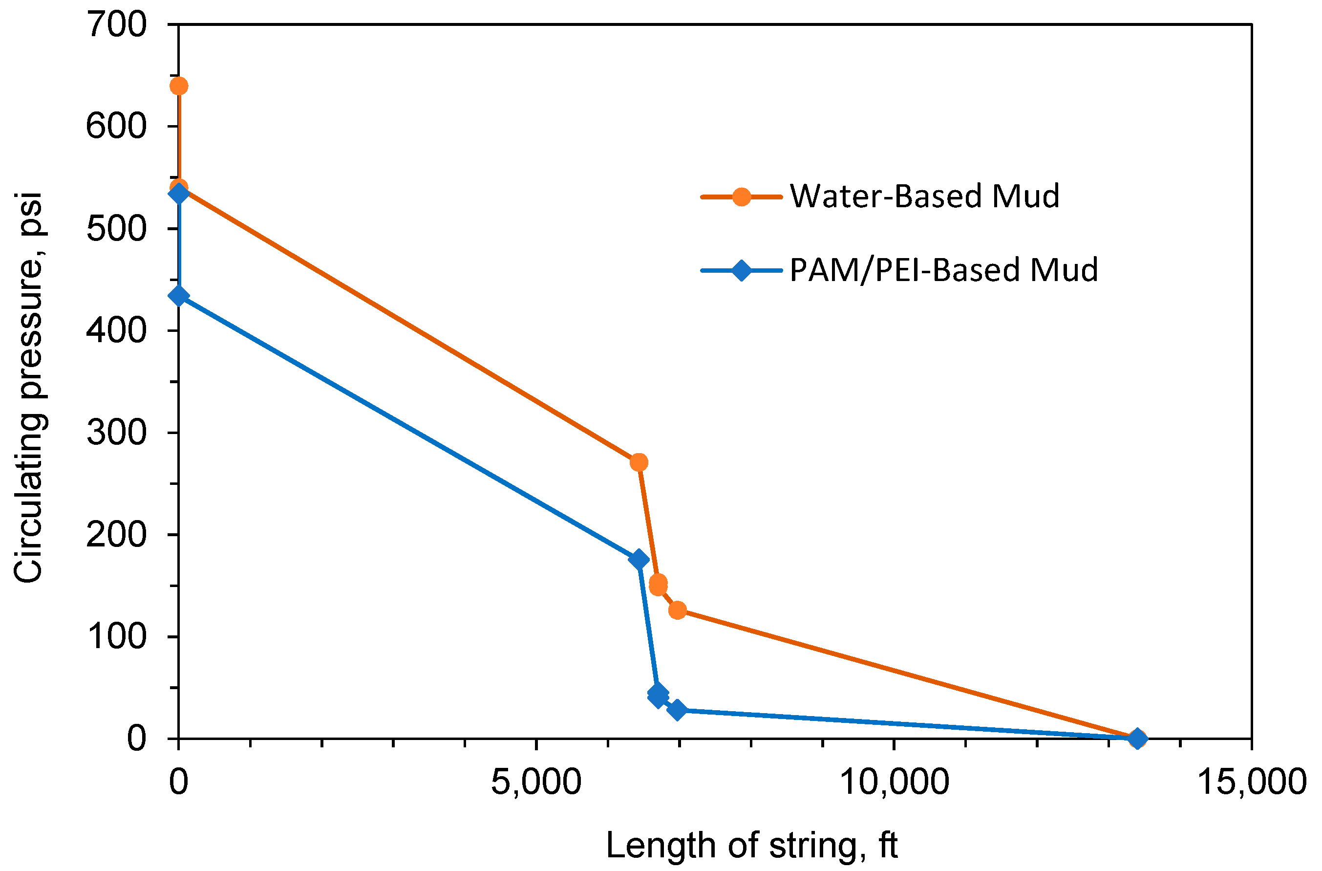
The experimental study presented in this paper, along with the developed machine learning approach, adds valuable information to help design the PAM/PEI mud system. The optimized concentration of PAM and other materials formulated a PAM/PEI-based mud of 9.5 ppg that resulted in 100 psi less circulating pressure. This reliable, highly accurate prediction of rheology that results from the interactions of polymers and the drilling fluid additives is important for hydraulic calculations and ECD management to prevent lost circulation.

References

- Ezeakacha, C.P.; Salehi, S. Experimental and statistical investigation of drilling fluids loss in porous media–part 1. J. Nat. Gas Sci. Eng. 2018, 51, 104–115. [Google Scholar] [CrossRef]
- Nygaard, R.; Salehi, S. Critical review of wellbore strengthening: Physical model and field deployment. In Proceedings of the AADE National Technical Conference and Exhibition, Houston, TX, USA, 12–14 April 2011. No. AADE-11-NTCE-24. [Google Scholar]
- Magzoub, M.I.; Salehi, S.; Hussein, I.A.; Nasser, M.S. Loss circulation in drilling and well construction: The sig-nificance of applications of crosslinked polymers in wellbore strengthening: A review. J. Pet. Sci. Eng. 2020, 185, 106653. [Google Scholar] [CrossRef]
- Salehi, S.; Madani, S.A.; Kiran, R. Characterization of drilling fluids filtration through integrated laboratory ex-periments and CFD modeling. J. Nat. Gas Sci. Eng. 2016, 29, 462–468. [Google Scholar] [CrossRef]
- Caenn, R.; Chillingar, G.V. Drilling fluids: State of the art. J. Pet. Sci. Eng. 1996, 14, 221–230. [Google Scholar] [CrossRef]
- Hamza, A.; Shamlooh, M.; Hussein, I.A.; Nasser, M.; Salehi, S. Polymeric formulations used for loss circulation materials and wellbore strengthening applications in oil and gas wells: A review. J. Pet. Sci. Eng. 2019, 180, 197–214. [Google Scholar] [CrossRef]
- El-karsani, K.S.M.; Al-Muntasheri, G.A.; Hussein, I.A. Polymer Systems for Water Shutoff and Profile Modifica-tion: A Review over the Last Decade. SPE J. 2014, 19, 135–149. [Google Scholar] [CrossRef]
- Rogovina, L.Z.; Vasil’ev, V.G.; Braudo, E.E. Definition of the concept of polymer gel. Polym. Sci. Ser. C 2008, 50, 85–92. [Google Scholar] [CrossRef]
- Ortiz Polo, R.P.; Monroy, R.R.; Toledo, N.; Dalrymple, E.D.; Eoff, L.; Everett, D. Field Applications of Low Molecular-Weight Polymer Activated with an Organic Crosslinker for Water Conformance in South Mexico. In Proceedings of the SPE Annual Technical Conference and Exhibition; Society of Petroleum Engineers, Houston, TX, USA, 26 September 2004; p. 5. [Google Scholar]
- Smith, J.E. Performance of 18 Polymers in Aluminum Citrate Colloidal Dispersion Gels, SPE International Sympo-Sium on Oilfield Chemistry; Society of Petroleum Engineers: San Antonio, TX, USA, 1995; p. 10. [Google Scholar]
- Al-Muntasheri, G.A.; Sierra, L.; Garzon, F.O.; Lynn, J.D.; Izquierdo, G.A. Water Shut-off with Polymer Gels in A High Temperature Horizontal Gas Well: A Success Story. In Proceedings of the SPE Improved Oil Recovery Symposium, Society of Petroleum Engineers, Tulsa, OK, USA, 11–13 April 2010; p. 24. [Google Scholar]
- Wastu, A.R.R.; Hamid, A.; Samsol, S. The effect of drilling mud on hole cleaning in oil and gas industry. J. Phys. Conf. Ser. 2019, 1402, 022054. [Google Scholar] [CrossRef]
- Igwilo, K.C.; Okoro, E.E.; Ohia, P.N.; Adenubi, S.A.; Okoli, N.; Adebayo, T. Effect of Mud Weight on Hole Cleaning During Oil and Gas Drilling Operations Effective Drilling Approach. Open Pet. Eng. J. 2019, 12, 14–22. [Google Scholar] [CrossRef]
- Khodja, M.; Canselier, J.P.; Bergaya, F.; Fourar, K.; Khodja, M.; Cohaut, N.; Benmounah, A. Shale problems and water-based drilling fluid optimisation in the Hassi Messaoud Algerian oil field. Appl. Clay Sci. 2010, 49, 383–393. [Google Scholar] [CrossRef] [Green Version]
- Bohloli, B.; de Pater, C. Experimental study on hydraulic fracturing of soft rocks: Influence of fluid rheology and confining stress. J. Pet. Sci. Eng. 2006, 53, 1–12. [Google Scholar] [CrossRef]
- Vajargah, A.K.; van Oort, E. Determination of drilling fluid rheology under downhole conditions by using re-al-time distributed pressure data. J. Nat. Gas Sci. Eng. 2015, 24, 400–411. [Google Scholar] [CrossRef]
- Steffe, J.F. Rheological Methods in Food Process Engineering, 2nd ed.; Freeman Press: Jackson, MI, USA, 1996. [Google Scholar]
- Paredes, J.C.B.; Lupo, C.; Escalera, H.M.; Medina, L.; Duno, H.; Zapata, J.G.; Tang, J.; Navarro, J.R.; Puerto, G.; Bedoya, J.; et al. Understanding Multiphase Flow Modeling for N2 Concentric Nitrogen Injection Through Downhole Pressure Sensor Data Measurements While Drilling MPD Wells. In Proceedings of the SPE/IADC Managed Pressure Drilling and Underbalanced Operations Conference and Exhibition; International Petroleum Technology Conference, San Antonio, TX, USA, 24–25 February 2010; p. 12. [Google Scholar]
- Liu, Y.; DiFoggio, R.; Hunnur, A.; Bergren, P.; Perez, L. Validation of Downhole Fluid Density, Viscosity and Sound Speed Sensor Measurements. In Proceedings of the SPWLA 54th Annual Logging Symposium. Society of Petrophysicists and Well-Log Analysts, New Orleans, LA, USA, 22 June 2013; p. 13. [Google Scholar]
- Kudaikulova, G. Rheology of drilling muds. J. Phys. Conf. Ser. 2015, 602, 012008. [Google Scholar] [CrossRef]
- Kister, E. Chemical Processing of the Drilling Fluids; Nedra, M., Ed.; Elsevier: Amsterdam, The Netherlands, 1972; p. 392. [Google Scholar]
- Du, H.; Wang, G.; Deng, G.; Cao, C. Modelling the effect of mudstone cuttings on rheological properties of KCl/Polymer water-based drilling fluid. J. Pet. Sci. Eng. 2018, 170, 422–429. [Google Scholar] [CrossRef]
- Shamlooh, M.; Hamza, A.; Hussein, I.A.; Nasser, M.S.; Magzoub, M.; Salehi, S. Investigation of the Rheological Properties of Nanosilica-Reinforced Polyacryla-mide/Polyethyleneimine Gels for Wellbore Strengthening at High Reservoir Temperatures. Energy Fuels 2019, 33, 6829–6836. [Google Scholar] [CrossRef]
- Magzoub, M.I.; Salehi, S.; Hussein, I.A.; Nasser, M.S. A Comprehensive Rheological Study for a Flowing Poly-mer-Based Drilling Fluid Used for Wellbore Strengthening. In Proceedings of the SPE International Conference and Exhibition on Formation Damage Control, Lafayette, LA, USA, 12 February 2020. [Google Scholar]
- Mohamed, A.I.; Hussein, I.A.; Sultan, A.S.; Al-Muntasheri, G.A. Gelation of emulsified polyacryla-mide/polyethylenimine under high-temperature, high-salinity conditions: Rheological investigation. Ind. Eng. Chem. Res. 2018, 57, 12278–12287. [Google Scholar] [CrossRef]
- Dhar, V.; Stein, R. Seven Methods for Transforming Corporate Data into Business Intelligence; Prentice-Hall, Inc.: Upper Saddle River, NJ, USA, 1997. [Google Scholar]
- Berry, M.J.; Linoff, G.S. Data Mining Techniques: For Marketing, Sales, and Customer Relationship Management; John Wiley & Sons: Hoboken, NJ, USA, 2004. [Google Scholar]
- Dhar, V. Data science and prediction. Commun. ACM 2013, 56, 64–73. [Google Scholar] [CrossRef]
- Xiuhua, Z.; Xiaochun, M. Drilling Fluids. 2010. Available online: https://dokumen.tips/documents/drilling-fluids-manual-important.html (accessed on 1 November 2010).
- Li, M.-C.; Wu, Q.; Song, K.; De Hoop, C.F.; Lee, S.; Qing, Y.; Wu, Y. Cellulose Nanocrystals and Polyanionic Cellulose as Additives in Bentonite Water-Based Drilling Fluids: Rheological Modeling and Filtration Mechanisms. Ind. Eng. Chem. Res. 2016, 55, 133–143. [Google Scholar] [CrossRef]
- Caenn, R.; Darley, H.C.; Gray, G.R. Composition and Properties of Drilling and Completion Fluids; Gulf Profes-Sional Publishing: Houston, TX, USA, 2011. [Google Scholar]
- Weikey, Y.; Sinha, S.L.; Dewangan, S.K. Advances in Rheological Measurement of Drilling Fluid—A Review. Prog. Petrochem. Sci. 2018, 2, 1–3. [Google Scholar] [CrossRef]
- Hegde, C.; Gray, K. Evaluation of coupled machine learning models for drilling optimization. J. Nat. Gas Sci. Eng. 2018, 56, 397–407. [Google Scholar] [CrossRef]
- Andaverde, J.; Wong-Loya, J.; Vargas-Tabares, Y.; Robles-Perez, M. A practical method for determining the rheology of drilling fluid. J. Pet. Sci. Eng. 2019, 180, 150–158. [Google Scholar] [CrossRef]
- Dullaert, K.; Mewis, J. A structural kinetics model for thixotropy. J. Non-Newton. Fluid Mech. 2006, 139, 21–30. [Google Scholar] [CrossRef]
- Skadsem, H.J.; Leulseged, A.; Cayeux, E. Measurement of drilling fluid rheology and modeling of thixotropic be-havior. Appl. Rheol. 2019, 29, 1–11. [Google Scholar] [CrossRef]
- Kiran, R.; Salehi, S. Assessing the Relation between Petrophysical and Operational Parameters in Geothermal Wells: A Machine Learning Approach. In Proceedings of the 45th Workshop on Geothermal Reservoir Engineering, Stanford, CA, USA, 7 October 2020; p. 13. [Google Scholar]
- Modaresi, F.; Araghinejad, S.; Ebrahimi, K. A comparative assessment of artificial neural network, generalized regression neural network, least-square support vector regression, and K-nearest neighbor regression for monthly stream-flow forecasting in linear and nonlinear conditions. Water Resour. Manag. 2018, 32, 243–258. [Google Scholar] [CrossRef]
- Poloczek, J.; Treiber, N.A.; Kramer, O. KNN Regression as Geo-Imputation Method for Spatio-Temporal Wind Data. In Proceedings of the Advances in Intelligent Systems and Computing, Canaria, Spain, 24–26 July 2014; pp. 185–193. [Google Scholar]
- Lin, Y.; Sun, Y. Grasp Mapping Using Locality Preserving Projections and kNN Regression. In Proceedings of the 2013 IEEE International Conference on Robotics and Automation, Karlsruhe, Germany, 6–10 May 2013; pp. 1076–1081. [Google Scholar]
- Onwuchekwa, C. Application of Machine Learning Ideas to Reservoir Fluid Properties Estimation. In Proceedings of the SPE Nigeria Annual International Conference and Exhibition, Lagos, Nigeria, 6 August 2018. [Google Scholar]
- Cover, T.; Hart, P. Nearest neighbor pattern classification. IEEE Trans. Inf. Theory 1967, 13, 21–27. [Google Scholar] [CrossRef]
- Alouhali, R.; Aljubran, M.; Gharbi, S.; Al-Yami, A. Drilling Through Data: Automated Kick Detection Using Data Mining. In Proceedings of the SPE International Heavy Oil Conference and Exhibition, Kuwait City, Kuwait, 10–12 December 2018. [Google Scholar]
- Belyadi, H.; McCallum, S.; Silva, F.; Carroll, O.; Weiman, S.; Smith, M. Production Prediction Using Multi-Output Supervised Machine Learning ML; Society of Petroleum Engineers (SPE): Tulsa, OK, USA, 2019. [Google Scholar]
- Dietterich, T.G. Ensemble Methods in Machine Learning, International Workshop on Multiple Classifier Systems; Springer: Berlin/Heidelberg, Germany, 2000; pp. 1–15. [Google Scholar]
- Breiman, L. Stacked regressions. Mach. Learn. 1996, 24, 49–64. [Google Scholar] [CrossRef] [Green Version]
- Shotton, J.; FitzGibbon, A.; Cook, M.; Sharp, T.; Finocchio, M.; Moore, R.; Kipman, A.; Blake, A. Real-time human pose recognition in parts from single depth images. In Proceedings of the CVPR 2011, Colorado Springs, CO, USA, 20–25 June 2011; pp. 1297–1304. [Google Scholar] [CrossRef] [Green Version]
- Svetnik, V.; Liaw, A.; Tong, C.; Culberson, J.C.; Sheridan, R.P.; Feuston, B.P. Random Forest: A Classification and Regression Tool for Compound Classification and QSAR Modeling. J. Chem. Inf. Comput. Sci. 2003, 43, 1947–1958. [Google Scholar] [CrossRef] [PubMed]
- Peters, J.; De Baets, B.; Verhoest, N.E.; Samson, R.; Degroeve, S.; De Becker, P.; Huybrechts, W. Random forests as a tool for ecohydrological distribution modelling. Ecol. Model. 2007, 207, 304–318. [Google Scholar] [CrossRef]
- Hegde, C.; Wallace, S.; Gray, K. Using Trees, Bagging, and Random Forests to Predict Rate of Penetration during Drilling. In Proceedings of the SPE Middle East Intelligent Oil and Gas Conference and Exhibition, 15 September 2015. [Google Scholar]
- Breiman, L. Random forests. Mach. Learn. 2001, 45, 5–32. [Google Scholar] [CrossRef] [Green Version]
- Zhang, Y.; Haghani, A. A gradient boosting method to improve travel time prediction. Transp. Res. Part C Emerg. Technol. 2015, 58, 308–324. [Google Scholar] [CrossRef]
- Friedman, J.H. Stochastic gradient boosting. Comput. Stat. Data Anal. 2002, 38, 367–378. [Google Scholar] [CrossRef]
- Natekin, A.; Knoll, A. Gradient boosting machines, a tutorial. Front. Neurorobot. 2013, 7, 21. [Google Scholar] [CrossRef] [PubMed] [Green Version]
- Friedman, J.H. Greedy function approximation: A gradient boosting machine. Ann. Stat. 2001, 1189–1232. [Google Scholar] [CrossRef]
- Hastie, T.; Tibshirani, R.; Friedman, J. The Elements of Statistical Learning: Data Mining, Inference, and Prediction; Springer: Berlin/Heidelberg, Germany, 2009. [Google Scholar]
- Torlay, L.; Perrone-Bertolotti, M.; Thomas, E.; Baciu, M. Machine learning–XGBoost analysis of language networks to classify patients with epilepsy. Brain Inform. 2017, 4, 159–169. [Google Scholar] [CrossRef] [PubMed]
- Freund, Y.; Schapire, R.E. Experiments with a New Boosting Algorithm. In Proceedings of the Thirteenth International Conference on International Conference on Machine Learning, Bari, Italy, 3–6 July 1996; Morgan Kaufmann Publishers Inc.: Bari, Italy, 1996; pp. 148–156. [Google Scholar]
- Freund, Y.; Shapire, R. A decision-theoretic generalization of on-line learning and an application to boosting. J. Comput. Syst. Sci. 1997, 55, 119–139. [Google Scholar] [CrossRef] [Green Version]
- Friedman, J.; Hastie, T.; Tibshirani, R. Additive logistic regression: A statistical view of boosting (with discussion and a rejoinder by the authors). Ann. Stat. 2000, 28, 337–407. [Google Scholar] [CrossRef]
- Lebanon, G.; Lafferty, J.D. Boosting and maximum likelihood for exponential models. Adv. Neural Infor-Mation Process. Syst. 2002, 14, 447–454. [Google Scholar]
- Madhuri, C.R.; Anuradha, G.; Pujitha, M.V. House Price Prediction Using Regression Techniques: A Comparative Study. In Proceedings of the 2019 International Conference on Smart Structures and Systems, Chennai, India, 14–15 March 2019; pp. 1–5. [Google Scholar]