
Elastic Energy Management Algorithm Using IoT Technology for Devices with Smart Appliance Functionality for Applications in Smart-Grid


1
Institute of Metrology, Electronics and Computer Science, University of Zielona Góra, 65-516 Zielona Gora, Poland
2
Institute of Automatic Control, Electronics and Electrical Engineering, University of Zielona Góra, 65-516 Zielona Gora, Poland
3
IHP-Leibniz Institute for High Performance Microelectronics, 15236 Frankfurt (Oder), Germany
*
Author to whom correspondence should be addressed.
Energies 2022, 15(1), 109; https://doi.org/10.3390/en15010109
Submission received: 9 November 2021
/
Revised: 14 December 2021
/
Accepted: 18 December 2021
/
Published: 23 December 2021
(This article belongs to the Special Issue Advances and Trends in Smart Energy Communities)
Abstract
:Currently, ensuring the correct functioning of the electrical grid is an important issue in terms of maintaining the normative voltage parameters and local line overloads. The unpredictability of Renewable Energy Sources (RES), the occurrence of the phenomenon of peak demand, as well as exceeding the voltage level above the nominal values in a smart grid makes it justifiable to conduct further research in this field. The article presents the results of simulation tests and experimental laboratory tests of an electricity management system in order to reduce excessively high grid load or reduce excessively high grid voltage values resulting from increased production of prosumer RES. The research is based on the Elastic Energy Management (EEM) algorithm for smart appliances (SA) using IoT (Internet of Things) technology. The data for the algorithm was obtained from a message broker that implements the Message Queue Telemetry Transport (MQTT) protocol. The complexity of selecting power settings for SA in the EEM algorithm required the use of a solution that is applied to the NP difficult problem class. For this purpose, the Greedy Randomized Adaptive Search Procedure (GRASP) was used in the EEM algorithm. The presented results of the simulation and experiment confirmed the possibility of regulating the network voltage by the Elastic Energy Management algorithm in the event of voltage fluctuations related to excessive load or local generation.
1. Introduction
Modern low-voltage power distribution networks are used not only to supply electricity to the end user, but also to receive electricity from local, prosumer Renewable Energy Sources (RES) [1,2]. As the process of changing the paradigm of the system operation was not related to its adaptation to the new realities, various technical problems have emerged [3,4]. These issues range from overvoltage, rapid voltage fluctuations, harmonics, protection coordination problems, energy flows into higher voltage grids, to transient stability.
The identified problems were mainly due to excess electricity in local balancing areas [2]. The excess of electric energy mainly causes a local voltage increase in the network above the normative values [5,6]. The voltage increase is caused by the positive voltage drop on the impedance of the distribution network caused by the current flow from RES [5,6,7]. The problem of increased voltage in the low voltage network can be solved by rebuilding the network using larger diameters of cables with lower impedance (lower voltage drops, but at the cost of large financial outlays) [3]. The second, more sensible solution, is the use of local energy storage, which would accumulate excess energy production from RES in the power grid [8,9,10]. This too is an expensive solution, the costs of which would be passed onto the prosumer. The technical solution for electricity distributor is the onload tap changer of distribution transformers [11]. Unfortunately, most countries do not have this type of regulation as standard in low voltage distribution networks. Reactive power management as well as reactive power generation by RES [12,13] or energy storage [14] is one of the methods of voltage regulation in the low voltage grid [12,13]. Another solution that would allow for voltage regulation in distribution networks is the so-called demand control [15,16] for the short-term balancing of the system so that the load power is close to the power generated from RES . There are many concepts for controlling the demand for electricity with the use of smart appliances described in the scientific literature, which will be described later in the introduction.
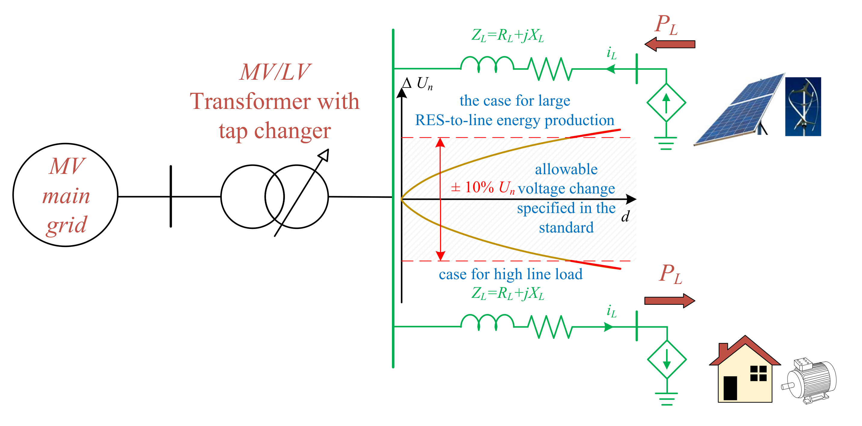
In addition to the increase in voltage caused by too much generation from RES, there are also problems with too low a voltage in the power system [5]. This is caused by excessively long radial distribution lines, often with too small a thickness of cables for the given load. However, the remedial measures proposed earlier are also adequate for solving problems with too low a voltage in the network. Figure 1 shows a schematic diagram of the influence of distributed generation and an excessive load on the voltage profile in the radial low voltage network. Low voltage networks are often dispersed over long distances. The distances d from the MV/LV transformer station determine the resultant impedances of the supply lines. If the network becomes too heavily loaded, there will be quite a large voltage drop across the line impedance. The voltage drop can be so large that the voltage value in the depths of the power grid will drop below the level allowed by the standards— (bottom part in Figure 1). In a situation where we have too much energy generation by RES in the electric power grid and too little local consumption of it, the voltage levels in the power grid may also increase beyond the limits allowed by the standards (top part in Figure 1). Voltage regulation of the power line by means of a tap changer is usually seasonal and selected in such a way as to ensure the nominal voltage level along its length. However, too high a generation of energy from RES in modern grids has meant that the regulation of the grid voltage by means of transformer taps is no longer sufficient.
This article will present the concept of the use and integration of smart home appliances and consumer devices in local low-voltage balancing of a distribution system in order to counteract the rise and fall of a network voltage. The smart appliances adopted in the article will be implemented in the Internet of Things (IoT) technology. In this article, we have adopted the definition of a smart appliance [17] as one which is characterized as a device that reacts to signals from its environment and working conditions. The concept of the smart device suggests that smart devices not only perform their main functionality in a user-defined manner, but also autonomously react to the environmental conditions in which they work. The main emphasis will be placed on balancing the supply of energy generated by RES in order to reduce transmission losses (thereby increasing the energy efficiency of the system), reduce grid voltage fluctuations (improving the reliability of the system and devices operating in it), and increase production from RES (by not switching off solar inverters during high voltage conditions of the supply network). Smart appliances will require users to change their behavior so that smart services can be provided [18].
As already mentioned in the introduction, many solutions for controlling the demand for electricity are described in the scientific literature. A short overview of selected applications for use with home appliances will be described below. The article [19] proposes an innovative Smart Load Node (SLN) approach to the efficient operation of non-intelligent household appliances in a smart grid environment. The proposed approach does not require any infrastructural changes in the electrical wiring or structural changes to household appliances at the production stage or by the consumer. The disadvantage of this solution is that SLN is meant to be connected between the existing power outlet and the load, though the device is complex as each SLN has a user interface that requires the consumer to configure the operation of a given load. The article [20] analyzes the problem of excessive network load by proposing an energy management system that automatically manages the Smart Home energy demand in accordance with network constraints and user priorities. The system is based on a heuristic technique that takes into account the user’s priority and the power available from the network and RES for device scheduling. The limitation of this approach is in its need to have information about the power available from the grid and about the power generated from PV (generally from RES). This complicates the governance system as there is no single leading signal about the state of the power system. The demonstration that the use of the Internet of Things (IoT) technology has a significant advantage over traditional communication technologies, but that it is still very rarely used in smart grid and smart home applications as shown in the article [21]. The authors have proposed, a holistic framework that includes various components from IoT architectures/frameworks to efficiently integrate smart appliances into an IoT cloud solution. An IoT typically consists of multiple Wireless Sensor Networks (WSN), which implies two major drawbacks of such a system: (1) The data is used only for local optimization and (2) the low cost-effectiveness of the solution. One of the proposed algorithms for scheduling the work of smart home devices in a given time period is presented in [22]. This algorithm is based on the mixed integers programming technique. The simulation results showed the effectiveness of the proposed solution in reducing electricity costs and the peak load. The article lacks information on how to obtain input data for effective regulation using the proposed approach. Socio-technical aspects related to the physical characteristics of devices, usage preferences, and user comfort requirements as well as their impact on the flexibility, acceptance, and effectiveness of demand response programs are described in the article [23]. The approach proposed in the article provides a framework for flexible planning at the device level, based on the self-determination of flexibility and comfort requirements by consumers. The findings of this paper confirm that consumers’ flexibility in appliance usage indeed varies across several socio-technical factors, such as applicant type, usage habits, and time of day. The problems faced by the operation of smart grid networks related to the management and processing of data in a reliable and secure manner, as well as communication problems such as latency, bandwidth, data overload, energy efficiency, etc., are described in the article [24]. A hybrid architecture based on the combination of fog computing and cloud computing has been proposed. This approach has been followed by handling real-time latency-sensitive information with high priority, cooperating with fog edge based servers deployed in close proximity to Home Area Networks (HANs). This approach was proposed for preprocessing and analyzing of information collected from smart IoT devices, such as smart appliances. The approach proposed in this article requires the use of advanced devices with 5G communication. The gradient boosting tree methodology with improved feature extraction is used in article [25] for the demand response framework to shift the grid load for residential applications. The proposed framework has several innovative features that model user satisfaction and the economic exploitation of a distributed household portfolio. The concept of using demand response with devices to reduce peak energy consumption, increase energy savings, turn on renewable energy sources, and reduce greenhouse gas emissions is an issue described in the article [26]. The advantage of the proposed approach is that the time-of-use valuation will allow for significant savings on the energy bills of the individual household. The article [27] proposes a new model, called the explicit-duration hidden Markov model with differential observations, for detecting and estimating the loads of individual household appliances on the basis of aggregated power signals collected by ordinary smart meters. This model was used to manage energy demand in a residential environment. The article only shows the results of simulation tests of the proposed estimation based on real data. The experiment will require the construction of a database with measurement data from energy meters. The concept of energy management based on the Elastic Energy Management algorithm (EEM) was presented in [28]. In this article, the results of simulation tests of the EEM algorithm were presented. The obtained results confirmed the possibility of adjusting the power of the SAs, so that the compromise between the user’s comfort and the requirements of the DSO operator was taken into account. It should be noted that the EEM algorithm in the research results took into account appropriately developed pricing programs. The article [29] presents a detailed price damage response model for a smart home with various types of household appliances, taking into account customer satisfaction. The proposed model takes into account various types of household appliances with different characteristics, as well as energy storage units and DER. The goal of minimizing energy expenditure, while fully taking into account user preferences in terms of comfort and lifestyle, requires the collection of a lot of data on user behavior. Not every user will be willing to disclose their preferences, so application of the approach may be limited. Finally, recent publications show that if instantaneous energy consumption data is provided to consumers as feedback shaping their behavior, about 20% of energy savings per household can be achieved. To achieve this goal, more detailed data is needed on the electricity consumed by each appliance, obtained through appliance load monitoring. Deep learning is the most famous and dynamically developing technique of artificial intelligence, which is indicated in [30] and solves the problem of identifying the acquisition of data on instantaneous energy consumption. It is an interesting issue from the point of view of science and the development of artificial intelligence methods [31]. The disadvantage of the proposed solutions is the high computational complexity and very specialized knowledge. However, a large part of the information can be obtained from the home devices themselves communicating via IoT protocols with the central control unit. Then, using the communication data, we can much more easily obtain information about not only the instantaneous energy demand by the SAs, but also information about the possibility of reducing energy consumption by a SA. This concept of electricity demand control will be the topic of this article. The presented literature review shows that there are many different methods of electricity demand management using SAs and the smart-home concept. It is a topical subject and indicates the high applicability of the proposed and interesting concepts.
The main aim of the article is to present the concept of an electricity management system in a smart home using SAs. The proposed system will use a control algorithm called the Elastic Energy Management algorithm (EEM). The result of the algorithm’s operation is energy management in the event of excess or lack of energy in the system (too much generation from RES or excessively loaded lines). An indirect effect of the algorithm is a voltage change in the power system. The line voltage increases as the line load is reduced, and the voltage drops as the line load increases. The presented system is based on a central unit that sends information to a SA with a request for the provision of a power reduction or line load service, if it has been programmed for such purposes by the user. Communication between the central unit and the SA takes place with the use of IoT protocols. In the proposed approach, the performed electricity demand management service will depend on the instantaneous value of the supply grid voltage. Depending on the level of deviation from the threshold values (lower or upper), the algorithm will either turn off the devices or reduce their power, or load the power grid by turning on loads that were previously defined by the user. The article presents a functional description of the proposed algorithm and its computational complexity. Then the simulation verification of the algorithm’s operation is carried out. The input data in the simulation investigation included: The measured voltages from the power grid, the measured power generated by the PV micro-installation, and the load profile defined by the authors. Additionally, an experimental verification of the functionality of the proposed system with the use of a laboratory simulation system will be presented. In experimental tests, SA devices will be simulated by a programmable load. The Message Queue Telemetry Transport (MQTT) protocol was created for the correct implementation of the algorithm on the Raspberry Pi 2 platform.
2. The Elastic Energy Management Algorithm
The EEM [28] was chosen to respond to voltage surges in the smart grid. This algorithm was developed to match energy demand and supply in energy systems. The actions taken by the EEM algorithm are aimed at ensuring a balance by reducing or increasing the power of intelligent receivers. The flowchart of the EEM algorithm is shown in Figure 2.
At the beginning of the operation of the EEM algorithm (Figure 2), data are collected. The acquired data is obtained from all available RESs () and all smart appliances (). It is also checked whether the DSO has submitted its request. If so, in this case the parameters will be defined: , , and . The EEM algorithm takes into account the current time t, so as to respond to a DSO service request (when ). Next, which functionality of the EEM algorithm will be triggered is checked: or . In conclusion, is called when it comes to providing user comfort, and when a request is made from the DSO.
This is due to the fact that there is a high level of energy production using RES, predominantly in short periods of time. EEM is also applicable when user actions lead to temporary above-average demand for energy. In the literature, this phenomenon is most often referred to as peak demand [32]. Commonly, such situations take place on hot days, during which there is a noticeable increase in energy demand by air conditioners.
Actions taken by the EEM algorithm can be triggered by the user or by control signals from the Distribution System Operator (DSO). In the case of the user, it will be due to the automation of the functioning of Smart Appliance (SA) behavior in the smart home. Automation will aim to optimize energy costs by depending on properly developed price programs, e.g., Real-time Pricing (RTP) and Time-of-Use (ToU). In [28], this variant of the EEM algorithm is designated as . In the case of DSO, the variant will have the task of modifying the power of the receivers to the level in the time interval requested by the DSO (, ) so that the difference between the sum of the power consumed by all appliances and the sum of the power supplied by the RES is not greater than . The main role of the EEM algorithm is to ensure user comfort while maintaining the lowest possible energy bills (). Additionally, at the request of the DSO, measures are taken to maintain the stability of the energy system ().
The actions that are taken by the EEM algorithm are related to two-way communication with intelligent devices, moreover control signals from the DSO are also taken into account (Figure 3).
Such communication is aimed at obtaining information about the status of a given device and sending control commands in the form of configuration parameters. For SA devices, the status is determined by the following parameters:
is the nominal value of the power at which the device operates. This value most often results from the design assumptions of a given type of device. P is the set of power selections. The number of settings P depends on the possibility of modifying the power settings of a given SA. If the set P is empty, it may mean that no power modification is possible for this particular device. Although it is not possible to modify the power for a device with an empty P set, reading such a status for the EEM algorithm will be used to determine the total demand for power by all devices. is a defined priority during power modification by the EEM algorithm. A three-stage scale is adopted for this parameter:
- ,
- ,
- .
In the case when , this means that power can be modified as much as possible. The values with the lowest priority are given to the SA in the case where the modification of the power settings will not affect the operation of the device. The SA will receive most often when modifications of power settings to devices with a lower priority will not bring the desired effect. The priority is assigned to devices for which power modification, e.g., for functional reasons could lead to the risk of human health or life, in extreme cases. The EEM algorithm for power modification of SAs with will be performed only in the case of critical events occurring in the Smart Grid (SG) network, e.g., natural disasters. is a defined time delay of device operation (hold). A device may have a status reported for a start-up but deferred. Such a function is known, inter alia, in household appliances, where the user sets a delay in starting, e.g., a dishwasher. The parameter means that the SA can be started later.
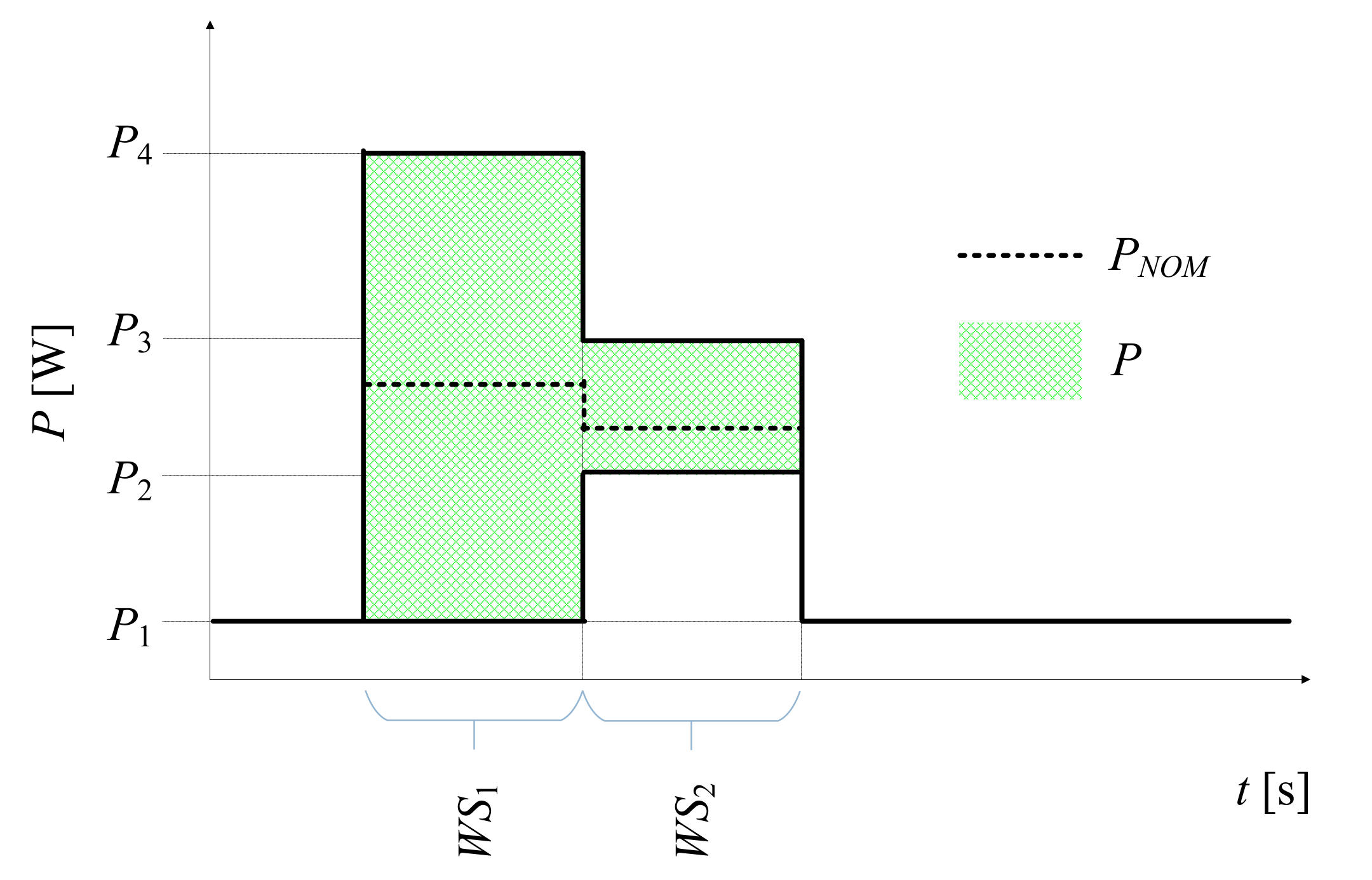
Parameters (1) result from the proposed description of the characteristics of SA functioning in [28]. The concept of worksection () is then introduced, denoting the selected phase of operation of a given SA, e.g., pre-washing, spinning, etc. An example of the parameters P and for two and is shown in Figure 4.
Independent ranges of power modification possibilities are marked for each . In , the range P may be modified within the range to , and in within the range to . When developing the assumptions for the EEM algorithm, devices that do not have a smart function were also taken into account. Such assumptions were made due to the fact that it was not possible to undertake actions on a mass scale aimed at replacing all devices with SA devices. Such an operation would be costly and could cause great social controversy. In the EEM algorithm, devices without smart functionality are therefore treated as generic devices without the possibility of influencing them with control operations.
In addition to SA devices, EEM also includes RES. For RES, only the status of the generated power is read using, e.g., Smart Inverter Communication Protocols [33].
The EEM algorithm also includes the verification of the voltage level in the network on the basis of data that would be provided by the DSO. It was assumed that the EEM algorithm would be designed to take action to lower or increase the load in the power grid when the ranges defined by the DSO are exceeded:
and are lower and upper ranges set by the voltage DSO and is the voltage in the SG.
The operation of EEM is based on the Greedy Randomized Adaptive Search Procedure (GRASP) heuristic algorithm, which allows the finding of the right solution (not necessarily the optimal one, but acceptable due to the cost of calculations) and is suitable for solving difficult NP problems.
In order to illustrate the scale of the complexity of the problem and the need to apply a heuristic algorithm to EEM, one of the simple examples of power selection for three SAs will be presented. In Figure 5, the ranges of power selection from to have been marked for each of the SAs and the value has been taken into account.
The ellipsis symbol marks other options for selecting a new power setting for a given SA. It is possible to check all possible combinations in Figure 5, but it will be very time consuming. Generally, determining the number of settings () for a given number of SAs is possible using the formula:
is for i-th SA defining the number of possible power choices and n – number of SAs.
Figure 6 shows for several examples of n. For the sake of simplification, an equal number of power selections was assumed for all SAs.
Based on Figure 6, it can be concluded that grows exponentially with the increase of . The value of is also significantly influenced by n. Such a way of increasing computational complexity can undoubtedly be classified as a Nondeterministic Polynomial time (NP problem). The GRASP algorithm requires the determination of the fitness function to function properly. The fitness function FEEM was developed for the EMM for the and variants:
, , and are components of the objective function related to DSO, SA, and RES, defined by formulas:
is the cost of purchasing 1 kWh from the DSO. i and j are respectively indices of SA and RES. and are numbers of RES and SA. is the power value after modification for the SA. is the nominal value of the power with which the SA works. is the cost of obtaining 1 kWh for a given RES. is the value of power obtained from a given RES. When U = 1, it means there is a balanced value of power demand for its supply. is the current value of power demand for its supply, calculated by the , based on selected values of appliance power, using the following equation:
is the maximum sum of power of all enabled consumers after the reduction process by , determined individually by the energy consumer. is for the variant which, due to the purpose of use other than , requires the adjustment of Formula (8) of SA power reduction over a specified period of time to a value at least equal to :
3. Simulation Research
The implementation of the software code for which the simulation tests were conducted was performed in Java in the Eclipse IDE [34]. During the implementation, apart from the solutions describing the EEM algorithm, functionalities that also enable the reading of configuration data and saving simulation results were taken into account. For the implemented solution, a diagram class was generated using the EclipseObjectAid UML Explorer [35] plug-in. The class diagram is shown in Figure 7.
Based on the diagram in Figure 7, it can be seen how the objects describing the SG network are created. For example, the class is inherited by the , , and classes. Subsequently, using these classes, it is possible to describe RES, conventional energy sources, and SA in simulation studies. For each SA using class , it is possible to assign a priority to .
For the purpose of conducting simulation tests for the EEM algorithm, the data used, the course of which is illustrated in Figure 8, was the value of voltage changes recorded in a real smart grid over one day.
Figure 8 shows the assumed range from = 220 [V] to = 247 [V], in which no additional actions are taken by the EEM algorithm. In the case of values outside the ranges, the load in the SG network will be increased or decreased in order to return the voltage to the range . Modification of the load in SG in the EEM algorithm will take place by increasing or decreasing the power of SA receivers. In the simulation tests performed, the reaction of the EEM algorithm resulting from exceeding the assumed range is marked with a red circle.
In order to increase the feasibility of the conducted simulation studies, the EEM algorithm was used as input data of the power generated from the photovoltaic installation (Figure 9). The choice of RES installation as a data source is to determine the EEM algorithm capabilities in households where an installation not exceeding 1 kW is installed. Due to the sunshine on the day of the measurements, the maximum value of the power supplied from the inverter did not exceed 631 [W] at 12:48. Data for 15 devices were provided as input to the EEM algorithm. The way of using individual devices was selected based on the authors’ own experience. An illustration of the operation of individual devices is shown in Figure 10.
Activation of individual receivers results from exemplary household activities, e.g., cooking, cleaning. These activities were treated as aperiodic tasks. In addition, also included are periodic tasks related to the start-up of devices in strictly defined time intervals. An example would be a refrigerator. In this case, the schedule of individual SAs runs can be equated with human appliance-usage patterns. The pattern results from the direct user action (e.g., cleaning) or the appliances specification (e.g., maintaining a certain temperature value in a refrigerator). Treating the use of equipment as periodic or aperiodic tasks extends the possibilities of using the EEM algorithm proposed in the article for adjusting power settings online. A smart energy meter would be a good place to allocate the EEM algorithm in this case. Such a meter would take into account aperiodic requests from DSO () and user comfort while optimizing energy costs () [28].
All necessary modifications of power settings to SA receivers are carried out in accordance with the adopted rules. It was assumed that each SA for each would be assigned the same . Table 1 summarizes the data on the assigned priorities.
For the fitness function (4), the value was adopted, denoting the balance between the household’s power demand and supply.
In the first test scenario, test scenario (S), it was assumed that each device is an SA device with the possibility of power regulation in the range from to . The value is understood to mean the power value which refers to the power value that is consumed by the device without SA functionality. In S1, it was assumed that for each SA it will be possible to modify the power in such a way that the SA can be completely turned off or it will be possible to increase its power twice .
Figure 11 shows the results of simulation tests for . In two series, the total power values were summarized for the case when the EEM algorithm was not run, i.e., , and when the total power was needed for SAs, i.e., when the power demand was modified by the EEM’s algorithm.
In for the series, a noticeable reduction in power demand is observed when the voltage value . In this case, the EEM algorithm sought to reduce the load in a given household. The adjustment achieved as a result of the SA power reduction is a compromise between maintaining the user’s comfort (when using SAs on a daily basis) and the requirements set by the DSO. In this case, it was about the need to reduce the power of those SAs for which it was possible. The level of power reduction for SAs took into account the power obtained at a given moment from RES (based on data in Figure 9). In order to fit the assumed voltage threshold from to (Figure 8), the was taken into account during the reduction. According to the markings in Figure 8, i.e., in selected time intervals, the EEM algorithm adjusted SA power only when it was needed ().
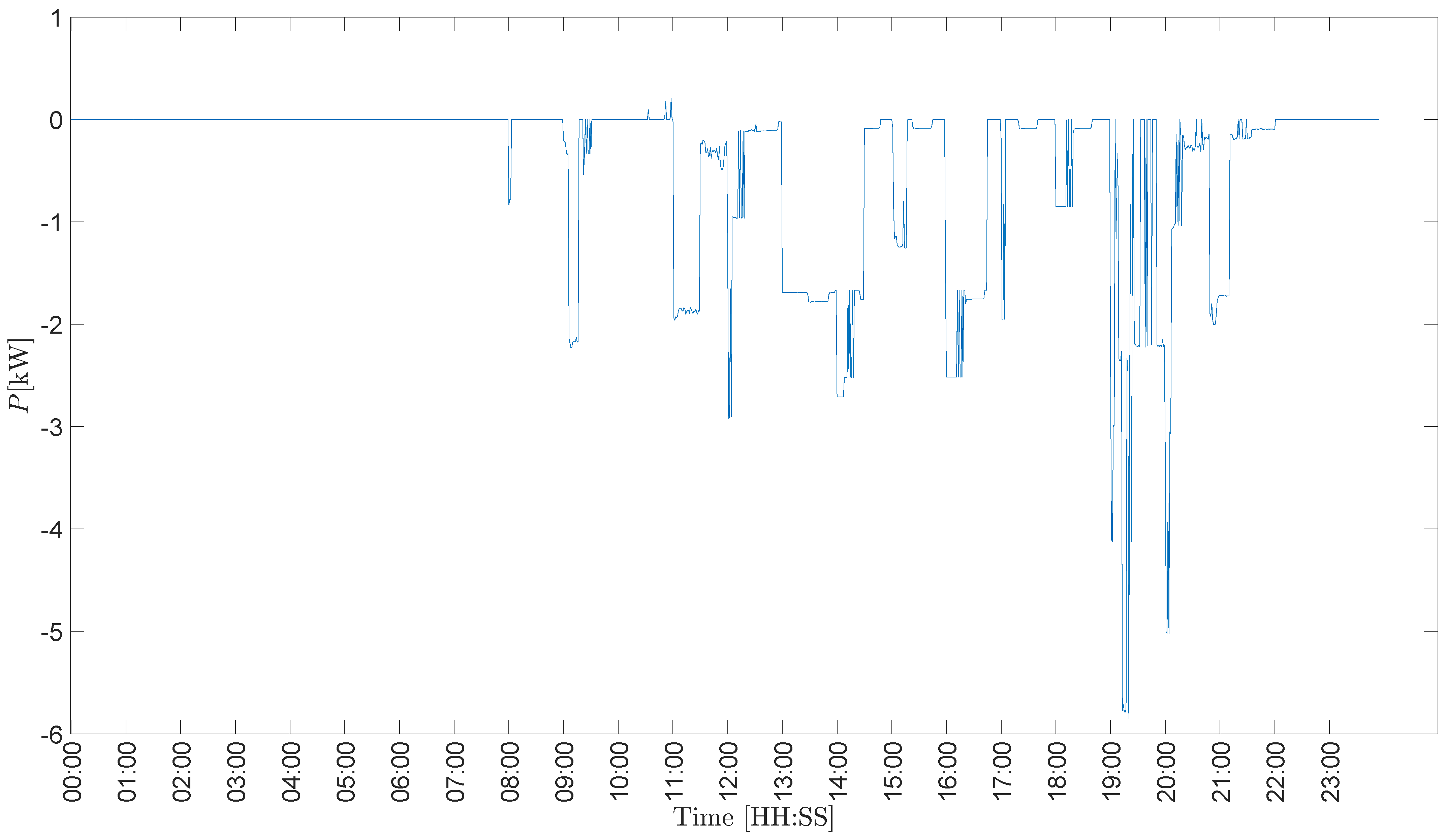
For a more detailed analysis of the results obtained from the EEM algorithm, the difference between and was determined. The results are shown in Figure 12.
In Figure 12, the presented difference and is intended to illustrate the situation when the EEM algorithm was working. In the case of negative values in the given time intervals, this meant a decrease in SA power, mainly as a result of exceeding the voltage value . The positive values obtained in Figure 12 define the situation when the EEM algorithm had to increase the power due to the fact of generation in RES. In each of these cases, modifying the power settings of the devices was required. Summarizing the EEM algorithm, using the available information from the devices, it was designed to ensure the maintenance of standard voltage parameters and local line overloads. The EEM algorithm mainly adjusts the SA’s power values to take into account the user’s comfort. First, the SAs that are least important to the user or conversely, the need for their correct operation are taken into account.
The aim of subsequent simulation studies was to determine the behavior of the EEM algorithm in a situation where the scope of possible SA power modifications would be mixed up. For this purpose, further S have been prepared, the assumptions of which are presented in Table 2.
Figure 13 summarizes the results of for S from Table 2 and, for comparison purposes, supplemented with the data from Figure 11.
Along with the decrease of the coefficient value, the scope of the possibility of modifying the settings for individual SAs decreased. In Figure 13, it is especially visible in the case of reducing SA power for the situation where . The values shown for for and are a special case. For for , which leads to a situation where neither of the SAs can modify the power settings.
In addition to the simulation tests themselves, the EEM algorithm was run in a test laboratory environment suitable for a small household, where several SA emulators would be located.
4. Research of the EEM Algorithm in a Test Laboratory Environment
The experimental setup includes the following devices:
Figure 14 shows a photo of the prepared test laboratory environment, while Figure 15 shows its electrical diagram.
Standalone applications running on the PC for power meter HIOKI PW3337 [36] and programmable AC Load 3091LD [37] were running on the PC. All data from and to these devices were saved on the MQTT Mosquitto server [39]. This server was running on a Raspberry Pi 2 board [38] and worked as a broker.
This software and hardware configuration enables scalability. Adding additional devices would only require the publishing of their data to the MQTT Mosquitto server [39] due to the support of the data transmission protocol for IoT [40]. Applying the IoT concept, it would be possible to ensure user comfort through the EEM algorithm that would introduce SA automation. Automation would contribute to reducing the cost of electricity [28]. It would also be possible to coordinate DSO activities when there is a need to reduce power, e.g., due to the phenomenon of peak demand [32].
An additional independent application running on a PC was an application that enabled the EEM algorithm to be operated. The algorithm was implemented in Java in the Eclipse IDE with thread support. Dedicated functionalities were implemented in the threads: The EEM algorithm and support for measurement and control devices. Due to the necessity to communicate with the MQTT Mosquitto server [39], the Paho library version 1.2.5 [41] was used. The implementation was run on a device with an embedded Raspberry Pi 2 system [38]. The MQTT Mosquitto server was configured to publish data about available smart applications and their parameters as well as the parameters of the smart grid. For the EEM algorithm, the following topic was defined on the MQTT Mosquitto server (Listing 1).
- Listing 1. Defined topic on the MQTT Mosquito server.
All data were published for a highest Quality of Service (QoS) level equal to 2. With this approach, it was guaranteed that all information about changes in individual values in a given topic would be provided. Additionally, the retained flag was set for each packet, which guarantees reading the last known message value for a given topic. In a given topic for a specific smart device, the following data was published in the paths (Listing 2).
- Listing 2. Defined topic for SAs.
In the path , it corresponds to the name of the smart appliance. The following parameters: , P, , and correspond to the meaning used in the EEM algorithm. In the case of status, information was added regarding whether the smart appliance was online or offline. For this, settings for the “Last Will and Testament” (LWT) for the connection were used. In the event that this client unexpectedly loses its connection to the server, the server will publish a message “offline”. Each publication of a parameter change for sets the status to online.
For the purpose of testing in a test laboratory environment, a configuration has been published for three SAs for one in the form of individual message values (Table 3).
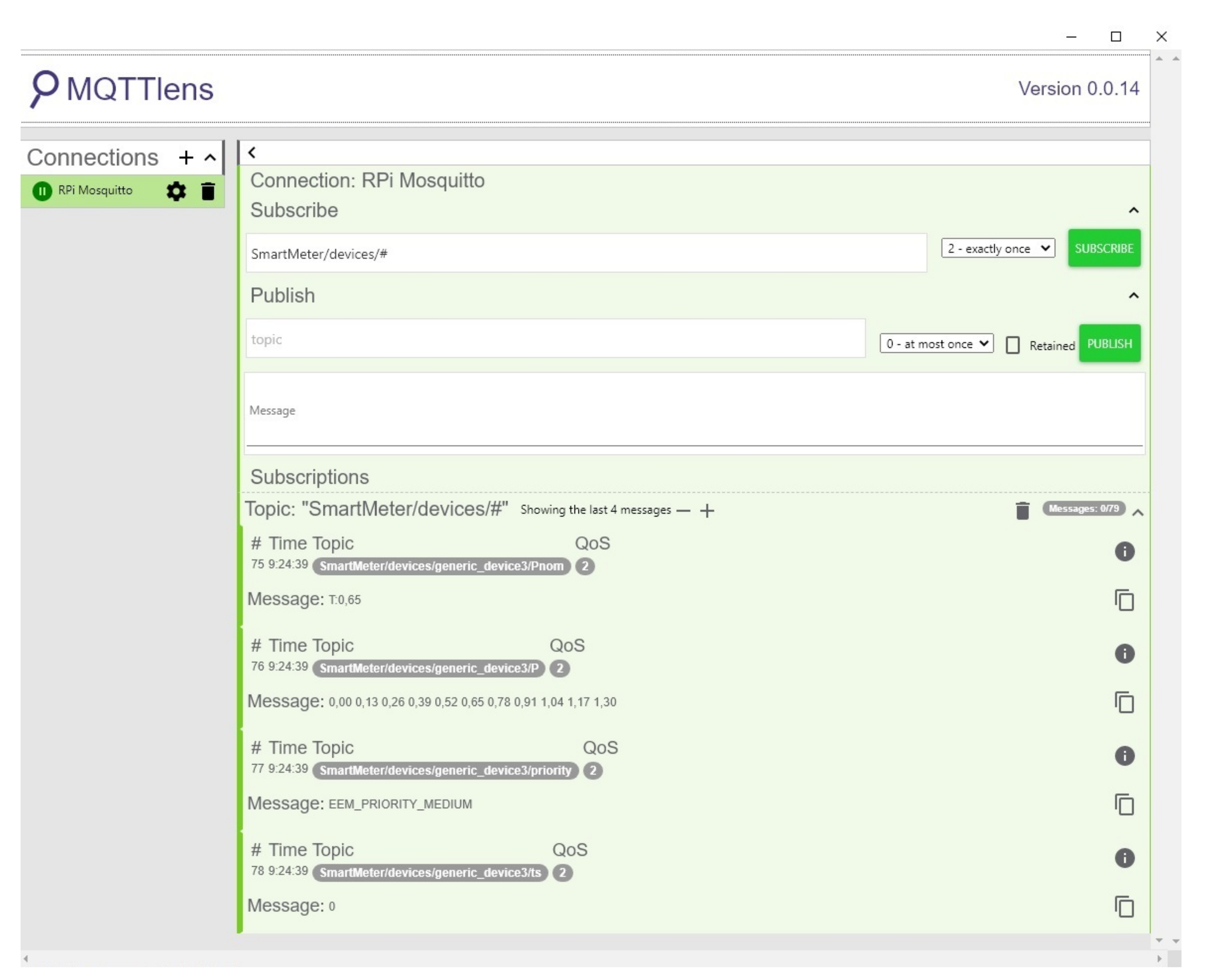
In order to verify the correctness of the data read from the MQTT server on the Raspberry Pi 2 [38], MQTTlens version 0.0.14 [42] was used. All topics were subscribed and delivered to the MQTT Mosquitto server. All changes were subscribed with a command, which is shown in (Listing 3). An example screen shot from MQTTlens application is shown in Figure 16.
- Listing 3. A command to subscribe topics.
Based on the data presented in Figure 16, it can be concluded that the connection to the Raspberry Pi2 was correctly set up. Additionally, the last four messages with data for the device named were read. These were the parameters specified in (1). The MQTT Mosquitto server also published data on the current voltage value in the test laboratory environment. For this purpose, an additional dedicated topic was defined (Listing 4).
- Listing 4. Additional defined topic for voltage.
The publication of the changed voltage values in the network in the test laboratory environment was carried out by a thread. The subscription to the changes has also been implemented in a separate thread. The threads are related to the support of two devices: HIOKI PW3337 Power meter and AC Load 3091LD. Communication between the PC and the HIOKI PW3337 and AC Load 3091LD Power meter was wired. Measurement and control commands in Standard Commands for Programmable Instruments (SCPI) were sent by wire. The HIOKI PW3337 power meter measured the mains voltage at the load terminals. The voltage value was published in the aforementioned topic (Listing 4). The mains voltage was adjusted manually with an autotransformer. After exceeding the set voltage limits, the EEM algorithm was activated.
Based on the value of the measurement voltage, the load was regulated in the test laboratory environment by means of AC Load 3091LD. The load regulation was to reflect the modification of the settings on one of the SA devices. The load value to be set was determined in the thread supporting the EEM algorithm. Regulation of the load current caused the voltage drop to change on the internal impedance of the autotransformer. Increasing the load current will cause a greater voltage drop, , which will result in a lower voltage at the load terminals. This corresponded to the situation in the real power grid when the grid voltage reached high values, e.g., caused by excessive generation of RES or underloading of the line. Then, the EEM algorithm proposed in the article activates the SAs that can be turned on or that the user has prepared for use in order to shift the load (e.g., washing machine, dishwasher, central heating boiler). On the other hand, reducing the load current causes a smaller voltage drop , which will result in an increase in voltage at the load terminals. This case will correspond to an excessively high load on the power network occurring, for example, during the morning peak load. Then the EEM algorithm will try to reduce the load by turning off the SAs that can be turned off at a given moment without losing the comfort of use or by reducing their power. Figure 17 and Figure 18 shows the results of the EEM algorithm testing in a test laboratory environment when it is necessary to modify the grid load due to exceeded voltage ranges.
Based on the analysis (Figure 17 and Figure 18) of the correlation between the voltage and load in the power grid, it can be concluded that if the , the EEM algorithm decreases the SA power, according to the available SA capacity as set out in Table 3. Increasing the SA power by EEM is performed when .
5. Conclusions
The concept of the system assumed the use of SA devices to control the amount of energy consumption from the power grid. With the use of such an approach, it is possible to both reduce the power grid at peak power loads, as well as increase the load on the power system due to excessively high power generation by pro-consumer RES systems. The line load status information for the proposed algorithm can be provided by various devices. In the article, the line load status is calculated on the basis of the line voltage level. If the voltage is too low, below the threshold set in the EEM algorithm, the line will be unloaded by disconnecting an SA, which may be disconnected at a given moment. In a situation when the voltage is too high, the SA will be turned on, which is set by the user as able to turn on, e.g., turning on the washing machine, dishwasher, heating domestic water or central heating, switching on cooking dinner, etc. Then the energy generated by RES is consumed and the line voltage is prevented from rising. The increase in line voltage causes the current from RES generators to flow through the impedance of the supply lines. Any changes to the power grid are posted on the MQTT Mosquitto server with broker functionality. Provision of information about changes is carried out by topic subscription. One of the subscribers in this case is the EEM algorithm. The presented results of experimental studies in a laboratory simulation system confirm the beneficial properties of such a regulation. The voltage was increased by about 5V by reducing the line load power, reducing the voltage drop on the impedance of the supply cable (autotransformer simulating a high impedance power grid). The voltage drop was also obtained by loading the system for the simulation of the system with a high voltage level.
Most of the research work has indicated a power loss in the distribution process and voltage profiles as major parameters in a behavioral study of a grid with a high number of RES. As mentioned in the introduction, the improvement of the voltage profile in the network can be performed with the use of various techniques. However, it should be remembered that the best way is to strike a balance between electricity production and demand. Extension of the structure of the elastic energy management system with new devices, e.g., RES inverters, electrical energy storage systems, or devices for distribution infrastructure will be the subject of further research. The new energy management structure with the use of an extended EEM will then allow energy management at the level of its production, storage and consumption, and response to changes in the voltage profile. This will allow an improvement in the balance between production and demand for electricity. Another issue of future research will be tests of the repeatability of its functioning at various levels of SA availability. Additionally, future activities will concern an examination of the functionality of the system and the correct operation of the proposed algorithm with the use of various input information such as: Weather data, historical data, RES generation data, line load data, etc. A greater number of input data used to control the system will increase the flexibility of regulation in various states of the power electronic system. Another interesting issue resulting from the structure of the system is the collection, transmission, and processing of measurement and control data. To increase the amount of data for the EEM algorithm, it will be necessary to use cloud computing. In this case, you may need to use virtual machines. Complex calculations would be performed on virtual machines, which would require a lot of computing power and a large amount of RAM. This approach would make it possible to easily scale the required hardware resources for computation [43]. We intend to create a comprehensive DSO solution that would cover more than just individual households. The EEM algorithm would enable the implementation of its functionalities and ensure user comfort and DSO requirements on devices available even in individual cities.
Author Contributions
Conceptualization, P.P., P.S. and K.P.; methodology, P.P., P.S. and K.P.; software, P.P.; validation, P.P. and P.S.; formal analysis, P.P. and P.S.; investigation, P.P. and P.S.; resources, P.P. and P.S.; data curation, P.P. and P.S.; writing—original draft preparation, P.P., P.S. and K.P.; writing—review and editing, P.P., P.S. and K.P.; visualization, P.P., P.S. and K.P.; supervision, P.P.; project administration, P.P.; funding acquisition, K.P. All authors have read and agreed to the published version of the manuscript.
Funding
This work was partially funded by the European Union within the European Regional Development Fund (ERDF), in the context of the INTERREG V A BB-PL Programme. Part of this work was carried out as part of the INTERREG Project on “Smart Grid Platform for research on energy management”, project number 85024423 as well as part of the H2020 ebalance plus project (grant number 864283).
Institutional Review Board Statement
Not applicable.
Informed Consent Statement
Not applicable.
Conflicts of Interest
The authors declare no conflict of interest.
Abbreviations
The following abbreviations are used in this manuscript:
| DSO | Distribution System Operator |
| EEM | Elastic Energy Management |
| GRASP | Greedy Randomized Adaptive Search Procedure |
| IoT | Internet of Things |
| LWT | Last Will and Testament |
| MQTT | Message Queue Telemetry Transport |
| RTP | Real-time pricing |
| RES | Renewable Energy Sources |
| SA | Smart Appliance |
| ToU | Time-of-Use |
| S | test scenario |
| SG | Smart Grid |
| WS | Work Section |
References
- Zhengyang, X.; Hong, L.; Hao, S.; Shaoyun, G.; Chengshan, W. Power supply capability evaluation of distribution systems with distributed generations under differentiated reliability constraints. Int. J. Electr. Power Energy Syst. 2022, 134, 107344. [Google Scholar] [CrossRef]
- Olek, B.; Wierzbowski, M. Local Energy Balancing and Ancillary Services in Low-Voltage Networks With Distributed Generation, Energy Storage, and Active Loads. IEEE Trans. Ind. Electron. 2015, 62, 2499–2508. [Google Scholar] [CrossRef]
- Iweh, C.D.; Gyamfi, S.; Tanyi, E.; Effah-Donyina, E. Distributed Generation and Renewable Energy Integration into the Grid: Prerequisites, Push Factors, Practical Options, Issues and Merits. Energies 2021, 14, 5375. [Google Scholar] [CrossRef]
- Meskin, M.; Domijan, A.; Grinberg, I. Impact of distributed generation on the protection systems of distribution networks: Analysis and remedies—Review paper. IET Gener. Transm. Distrib. 2020, 14, 5944–5960. [Google Scholar] [CrossRef]
- Hashemi, S.; Østergaard, J. Methods and strategies for overvoltage prevention in low voltage distribution systems with PV. IET Renew. Power Gener. 2017, 11, 205–214. [Google Scholar] [CrossRef] [Green Version]
- Ramadhani, U.H.; Fachrizal, R.; Shepero, M.; Munkhammar, J.; Widén, J. Probabilistic load flow analysis of electric vehicle smart charging in unbalanced LV distribution systems with residential photovoltaic generation. Sustain. Cities Soc. 2021, 72, 103043. [Google Scholar] [CrossRef]
- Zarco-Soto, F.J.; Zarco-Periñán, P.J.; Martínez-Ramos, J.L. Centralized Control of Distribution Networks with High Penetration of Renewable Energies. Energies 2021, 14, 4283. [Google Scholar] [CrossRef]
- Luo, X.; Wang, J.; Dooner, M.; Clarke, J. Overview of current development in electrical energy storage technologies and the application potential in power system operation. Appl. Energy 2015, 137, 511–536. [Google Scholar] [CrossRef] [Green Version]
- Masebinu, S.O.; Akinlabi, E.T.; Muzenda, E.; Aboyade, A.O. Techno-economic analysis of grid-tied energy storage. Int. J. Environ. Sci. Technol. 2018, 15, 231–242. [Google Scholar] [CrossRef]
- Arteaga, J.; Zareipour, H.; Amjady, N. Energy Storage as a Service: Optimal sizing for Transmission Congestion Relief. Appl. Energy 2021, 298, 117095. [Google Scholar] [CrossRef]
- Aziz, T.; Ketjoy, N. Enhancing PV Penetration in LV Networks Using Reactive Power Control and On Load Tap Changer With Existing Transformers. IEEE Access 2018, 6, 2683–2691. [Google Scholar] [CrossRef]
- Majumder, R. Aspect of voltage stability and reactive power support in active distribution. IET Gener. Transm. Distrib. 2014, 8, 442–450. [Google Scholar] [CrossRef]
- Yang, D.; Wang, X.; Liu, F.; Xin, K.; Liu, Y.; Blaabjerg, F. Adaptive Reactive Power Control of PV Power Plants for Improved Power Transfer Capability Under Ultra-Weak Grid Conditions. IEEE Trans. Smart Grid 2019, 10, 1269–1279. [Google Scholar] [CrossRef] [Green Version]
- Felipe, J.; Zimann, A.L.; Batschauer, M.M.; Neves, F. Energy storage system control algorithm for voltage regulation with active and reactive power injection in low-voltage distribution network. Electr. Power Syst. Res. 2019, 174, 105825. [Google Scholar] [CrossRef]
- Siano, P. Demand response and smart grids—A survey. Renew. Sustain. Energy Rev. 2014, 30, 461–478. [Google Scholar] [CrossRef]
- Jabir, H.J.; Teh, J.; Ishak, D.; Abunima, H. Impacts of Demand-Side Management on Electrical Power Systems: A Review. Energies 2018, 11, 1050. [Google Scholar] [CrossRef] [Green Version]
- Schmidt, A.; van Laerhoven, K. How to build smart appliances? IEEE Pers. Commun. 2001, 8, 66–71. [Google Scholar] [CrossRef]
- Zhai, S.; Wang, Z.; Yan, X.; He, G. Appliance Flexibility Analysis Considering User Behavior in Home Energy Management System Using Smart Plugs. IEEE Trans. Ind. Electron. 2019, 66, 1391–1401. [Google Scholar] [CrossRef]
- Singh, S.; Roy, A.; Selvan, M.P. Smart Load Node for Nonsmart Load Under Smart Grid Paradigm: A New Home Energy Management System. IEEE Consum. Electron. Mag. 2019, 8, 22–27. [Google Scholar] [CrossRef] [Green Version]
- Jindal, A.; Bhambhu, B.S.; Singh, M.; Kumar, N.; Naik, K. A Heuristic-Based Appliance Scheduling Scheme for Smart Homes. IEEE Trans. Ind. Informatics 2020, 16, 3242–3255. [Google Scholar] [CrossRef] [Green Version]
- Biljana, L.; RisteskaStojkoska, K.; Trivodaliev, V. A review of Internet of Things for smart home: Challenges and solutions. J. Clean. Prod. 2017, 140, 1454–1464. [Google Scholar] [CrossRef]
- Qayyum, F.A.; Naeem, M.; Khwaja, A.S.; Anpalagan, A.; Guan, L.; Venkatesh, B. Appliance Scheduling Optimization in Smart Home Networks. IEEE Access 2015, 3, 2176–2190. [Google Scholar] [CrossRef]
- Fanitabasi, F.; Pournaras, E. Appliance-Level Flexible Scheduling for Socio-Technical Smart Grid Optimization. IEEE Access 2020, 8, 119880–119898. [Google Scholar] [CrossRef]
- Molokomme, D.N.; Chabalala, C.S.; Bokoro, P.N. A Review of Cognitive Radio Smart Grid Communication Infrastructure Systems. Energies 2020, 13, 3245. [Google Scholar] [CrossRef]
- Bintoudi, A.D.; Bezas, N.; Zyglakis, L.; Isaioglou, G.; Timplalexis, C.; Gkaidatzis, P.; Tryferidis, A.; Ioannidis, D.; Tzovaras, D. Incentive-Based Demand Response Framework for Residential Applications: Design and Real-Life Demonstration. Energies 2021, 14, 4315. [Google Scholar] [CrossRef]
- Lui, T.J.; Stirling, W.; Marcy, H.O. Get Smart. IEEE Power Energy Mag. 2010, 8, 66–78. [Google Scholar] [CrossRef]
- Guo, Z.; Wang, Z.J.; Kashani, A. Home Appliance Load Modeling From Aggregated Smart Meter Data. IEEE Trans. Power Syst. 2015, 30, 254–262. [Google Scholar] [CrossRef] [Green Version]
- Powroźnik, P.; Szulim, R.; Miczulski, W.; Piotrowski, K. Household Energy Management. Appl. Sci. 2021, 11, 1626. [Google Scholar] [CrossRef]
- Liu, Y.; Xiao, L.; Yao, G.; Bu, S. Pricing-Based Demand Response for a Smart Home With Various Types of Household Appliances Considering Customer Satisfaction. IEEE Access 2019, 7, 86463–86472. [Google Scholar] [CrossRef]
- Cimen, H.; Palacios-Garcia, E.J.; Kolaek, M.; Cetinkaya, N.; Vasquez, J.C.; Guerrero, J.M. Smart-Building Applications: Deep Learning-Based, Real-Time Load Monitoring. IEEE Ind. Electron. Mag. 2021, 15, 4–15. [Google Scholar] [CrossRef]
- Foukalas, F.; Tziouvaras, A. Edge Artificial Intelligence for Industrial Internet of Things Applications: An Industrial Edge Intelligence Solution. IEEE Ind. Electron. Mag. 2021, 15, 28–36. [Google Scholar] [CrossRef]
- Delberis, A.L.; Andrés, M.C.G.; Érica, T.; Eidy, M.M.B. Peak demand contract for big consumers computed based on the combination of a statistical model and a mixed integer linear programming stochastic optimization model. Electr. Power Syst. Res. 2018, 154, 122–129. [Google Scholar] [CrossRef]
- Smart Inverter Communication Protocols. Available online: https://www.intertek.com/blog/2019-05-24-inverter/ (accessed on 12 September 2021).
- Eclipse IDE and Web IDEs. Available online: https://www.eclipse.org/ide/ (accessed on 1 July 2021).
- ObjectAid UML Explorer. Available online: https://marketplace.eclipse.org/content/objectaid-uml-explorer/ (accessed on 1 July 2021).
- Power Meter HIOKI PW3337. Available online: https://www.hioki.com/global/products/power-meters/3phase-ac-dc/id_5929 (accessed on 1 May 2021).
- AC Load 3091LD. Available online: https://www.powerandtest.com/power/electronic-loads/ac-electronic-load-3091ld (accessed on 1 May 2021).
- Raspberry Pi 2. Available online: https://www.raspberrypi.com/products/raspberry-pi-2-model-b/ (accessed on 1 May 2021).
- MQTT Mosquitto Server. Available online: https://mosquitto.org/ (accessed on 1 May 2021).
- Khan, M.A.; Khan, M.A.; Jan, S.U.; Ahmad, J.; Jamal, S.S.; Shah, A.A.; Pitropakis, N.; Buchanan, W.J. A Deep Learning-Based Intrusion Detection System for MQTT Enabled IoT. Sensors 2021, 21, 7016. [Google Scholar] [CrossRef] [PubMed]
- Paho Library Version 1.2.5. Available online: https://www.eclipse.org/paho/index.php?page=clients/java/index.php (accessed on 1 May 2021).
- MQTTlens Version 0.0.14. Available online: https://chrome.google.com/webstore/detail/mqttlens/hemojaaeigabkbcookmlgmdigohjobjm (accessed on 1 May 2021).
- Khan, A.A.; Zakarya, M.; Khan, R. Energy-aware dynamic resource management in elastic cloud datacenters. Simul. Model. Pract. Theory 2019, 92, 82–99. [Google Scholar] [CrossRef]
Figure 1.
Influence of the line impedance in the low-voltage network on the voltage profile for lines with high Renewable Energy Sources (RES) penetration and for lines with high loads.
Figure 1.
Influence of the line impedance in the low-voltage network on the voltage profile for lines with high Renewable Energy Sources (RES) penetration and for lines with high loads.

Figure 2.
Flowchart of the EEM algorithm.

Figure 3.
Illustration of data exchange between the EEM algorithm from DSO and SA in HAN.

Figure 4.
Graphical presentation of parameters that define SA.

Figure 5.
An example of presenting the complexity of the power selection options for three SAs.

Figure 6.
Determination of for the selected number of SA (n) and possible power choices .

Figure 7.
Class diagram for the implemented EEM algorithm.

Figure 8.
Examples of U values with marked threshold ranges and .

Figure 9.
Sample data from a photovoltaic installation.

Figure 10.
Sample SAs schedule.

Figure 11.
Research results for .

Figure 12.
Determining the time when the EEM algorithm worked, based on the difference and .

Figure 13.
Simulation test results for all defined S.

Figure 14.
Photo of the laboratory experimental setup: 1—autotransformer, 2—programmable AC Load 3091LD, 3—power meter HIOKI PW3337, 4—Raspberry Pi 2, and 5—PC computer.
Figure 14.
Photo of the laboratory experimental setup: 1—autotransformer, 2—programmable AC Load 3091LD, 3—power meter HIOKI PW3337, 4—Raspberry Pi 2, and 5—PC computer.

Figure 15.
Schematic diagram of experimental setup.

Figure 16.
MQTTlens application.

Figure 17.
Results from test laboratory environment for increasing .

Figure 18.
Results from test laboratory environment for decreasing .


Table 1.
List of SAs and their assigned values.
| SA | |
|---|---|
| laptop | |
| kettle | |
| washing machine | |
| vacuum cleaner | |
| tv | |
| refrigerator | |
| dishwasher | |
| iron | |
| boiler | |
| oven | |
| air conditioner | |
| microwave | |
| coffee machine | |
| cooker hood | |
| electric cooker |
Table 2.
List of S parameters for subsequent simulation research.
| S | c |
|---|---|
| 90 | |
| 75 | |
| 50 | |
| 25 | |
| 10 | |
| 0 |
1 where c-percentage range coefficient.
Table 3.
List of parameters adopted for research.
| Device Name | P | |||
|---|---|---|---|---|
| 0.00, 0.29, 0.58, 0.87, 1.16, 1.45, 1.74, 2.03, 2.32, 2.61, 2.90 | 1.45 | 0 | ||
| 0.00, 0.17, 0.34, 0.51, 0.68, 0.85, 1.02, 1.19, 1.36, 1.53, 1.70 | 0.85 | 0 | ||
| 0.00, 0.13, 0.26, 0.39, 0.52, 0.65, 0.78, 0.91, 1.04, 1.17, 1.30 | 0.65 | 0 |
Publisher’s Note: MDPI stays neutral with regard to jurisdictional claims in published maps and institutional affiliations. |
© 2021 by the authors. Licensee MDPI, Basel, Switzerland. This article is an open access article distributed under the terms and conditions of the Creative Commons Attribution (CC BY) license (https://creativecommons.org/licenses/by/4.0/).
Share and Cite
MDPI and ACS Style
Powroźnik, P.; Szcześniak, P.; Piotrowski, K. Elastic Energy Management Algorithm Using IoT Technology for Devices with Smart Appliance Functionality for Applications in Smart-Grid. Energies 2022, 15, 109. https://doi.org/10.3390/en15010109
AMA Style
Powroźnik P, Szcześniak P, Piotrowski K. Elastic Energy Management Algorithm Using IoT Technology for Devices with Smart Appliance Functionality for Applications in Smart-Grid. Energies. 2022; 15(1):109. https://doi.org/10.3390/en15010109
Chicago/Turabian StylePowroźnik, Piotr, Paweł Szcześniak, and Krzysztof Piotrowski. 2022. "Elastic Energy Management Algorithm Using IoT Technology for Devices with Smart Appliance Functionality for Applications in Smart-Grid" Energies 15, no. 1: 109. https://doi.org/10.3390/en15010109
Note that from the first issue of 2016, this journal uses article numbers instead of page numbers. See further details here.