
Contributions to Power Management in AC Microgrids Based on Concepts of Microeconomics Theory
by
 , , , and
Luís F. R. Pinto
1 ,
,
Tiago D. C. Busarello
2 ,
,
Lucas V. Bellinaso
3 ,
,
Leandro Michels
3 and
Marcello Mezaroba
1,* 1
Department of Electrical Engineering, Santa Catarina State University, Joinville 89219-710, Brazil
2
Department of Control, Automation and Computing Engineering, Federal University of Santa Catarina, Blumenau 89036-004, Brazil
3
Power Electronics and Control Research Group (GEPOC), Federal University of Santa Maria, Santa Maria 97105-900, Brazil
*
Author to whom correspondence should be addressed.
Energies 2022, 15(11), 3890; https://doi.org/10.3390/en15113890
Submission received: 29 March 2022
/
Revised: 11 May 2022
/
Accepted: 14 May 2022
/
Published: 25 May 2022
(This article belongs to the Special Issue Control of Distributed Power Electronic Converters in Smart Energy Systems)
Abstract
:Renewable energy sources are growing in importance and reshaping power systems through microgrid (MG) networks. Some relevant issues in the management of an MG need to be addressed, such as voltage and frequency control, power balance between sources (sharing) and distributed loads, stability, security, power quality, etc. As a contribution, this manuscript presents a power management of AC MGs based on concepts of microeconomics theory for market equilibrium. The prices of active and reactive energy are informed through the AC voltage parameters such as magnitude, frequency and angle. This approach allows several sources and loads to operate with no extra communication interface. Experiments are provided to validate operation in many different operational scenarios using a hardware-in-the-loop environment.
1. Introduction
The demand for electrical energy is growing and trending to become one of the main sources of power in the near future. The traditional Electric Power System (EPS) is being replaced, which is mainly due to the shortage of fossil fuels, carbon emissions, long construction time, high transmission losses, low efficiency, higher cost, reduced reliability, etc. New challenges are emerging in EPSs; centralized power generation is changing as well as transmission and distribution. Innovations in distributed generation (DG), or distributed energy resources (DERs), which use different renewable resources, such as solar photovoltaic, wind, micro-hydro, fuel cell, microturbine and others, with a decentralized EPS, are the most effective response to this new situation. An MG can be defined as an integrated system composed of DERs operating as a single system that can operate connected to or islanded from the main grid [1,2,3,4]. MGs are a promising approach for many EPSs to achieve better efficiency and reliability. They can be classified by how the DERs are interconnected: DC, AC, or mixed [5,6]. A DC bus MG presents some advantages such as simplicity, high reliability, absence of reactive control, and absence of synchronization requirements [5]. On the other hand, an AC MG has simpler voltage transformations, easy galvanic insulation, and cheaper protection devices, and it can be easily integrated to the AC power grid [1,7].
One of the challenges for MGs is their operating control. An MG control can be organized in three hierarchical levels. The primary level is associated with the inverter’s internal control schemes [4,8] for voltage, current and frequency, which are tracked against a reference through a closed-loop control scheme. The goal is to improve voltage regulation, reliability, stability, and power sharing while not requiring any communication aspects [9,10]. The main existing control schemes are proportional integral (PI), angle droop control, P/fdroop, P/Vdroop, virtual impedance loop, and many others. The secondary level functions to restore the MG voltage and frequency to the nominal values [11,12]. When the load on the MG bus changes, so do the voltage and frequency, which must be brought back to their nominal values. To do so, the MG supervisory system must send a reference signal to each MG unit, using a low-bandwidth communication system. This control can also be used to synchronize the MG with the grid before the interconnection, when changing from islanded to connected mode [13,14]. The main existing control schemes are the Multi-Agent System (MAS), Consensus-Based Control, Model Predictive Control, etc. The tertiary level is related to an Energy Management System (EMS) and regulates the power flow between the grid and the MG [15,16,17]. It also optimizes the MG operation in both modes, acting on the voltage and internal frequency reference, following the operational plan established by the MG administrator. Examples of tertiary-level control techniques are cited in [18], showing the Energy Management System, Optimization System and Power Flow Operation, among others. A dynamic view of those three levels shows that the primary level is always adjusting the power sharing of each source in relation to the others and to the demand on the MG bus. Deviations can occur in voltage and frequency on the bus, and the secondary control level is responsible for bringing them back to the MG reference values. The tertiary control level changes the MG operating setpoints to adjust the power flow between it and the grid as specified by the microgrid administrator, since it is up to him/her to determine how much power can be made available or will have to be absorbed.
The literature on the state of the art in MG control methods, which has been covered with many examples by [19,20], presents many possibilities for improvement. The Power Management System in an MG must consider stability, protection, power balance, mode transitions, power exchange with the grid, synchronization and power optimization. Many strategies have been developed to achieve such purposes, which can been classified according to their management control scheme: centralized or non-centralized [21]. Centralized approaches, whose main techniques are Power Sharing [12] and Optimal Power Flow [22,23], assume that the management of MGs is performed from a central controller located at the global control level. Non-centralized approaches cover many techniques, such as Multi-Agent System [24], Normal Average [25], and Consensus Based [23], as well as decentralized ones. Decentralized approaches are AC Bus Signaling (ABS) [26], DC voltage Bus Signaling (DBS) [27], and Virtual impedance [10], among others [28]. The ABS considers voltage-level changes in the AC bus [29]. It presents the advantage of allowing the implementation of a distributed control scheme with the same reliability of a decentralized one [26,27,30].
Regarding the current development of MGs and their future role in new electrical grids, according to [14] the road map of new developments in microgrids can be grouped into three main areas, which are closely linked to each other: (1) network integration of electrical Energy Storage Systems (EES) into microgrids and power generation facilities, (2) active demand management, and (3) improved controllability and monitoring of MGs. The same researcher adds that an important area for future development is energy storage, and a second area in which relevant contributions are soon expected to emerge is related to the active management of demand and supply, that is, the active coordination of distributed consumers and generators to optimize energy use and energy flow.
This manuscript proposes a power management approach for AC MGs based on the microeconomic theory of market equilibrium [31]. An internal price is used, considering that energy and money exchanges are carried out with multiple users who pay (loads) or receive (sources) according to such price. A dynamic pricing scheme is adopted, as it may be more efficient at enabling demand response (DR) actions than other pricing-based schemes (such as fixed or time-of-use (TOU) pricing) [32]. When power is abundant, the price drops, and when it is scarce, the price rises. The main contribution of this manuscript is in power management, using a non-centralized approach, for many plug and play units. It is scalable, since the more units, the better the performance [21], and it is equally applicable for any unit, be it supply, load, storage or another MG, with the possibility to keep running even without the communication link. As it uses the same principle to manage the active and the reactive power, it is recommended for AC, DC or a mixed MG, with robustness and low cost, while giving the user more autonomy.
The voltage level is used to inform the active power price, since the application is assumed for low-voltage MGs concentrated in a small area where grid impedance is predominantly resistive. The reactive power price is informed by the angle between the grid and the point of common coupling (PCC) in grid-tie mode or by the frequency in island mode. Based on that information, a decision algorithm in the non-centralized controller commands the DERs to connect or disconnect. To validate the proposed approach, the algorithms were implemented in the DSPs of DER controllers. Experimental results were obtained with a Typhoon HIL 402 hardware-in-the-loop(HIL) device, emulating the real-time dynamic behavior of an MG, with grid-tied and off-grid operating modes.
2. Materials and Methods
2.1. MG Management Strategy
The strategy was based on and adapted from [33,34], which is based on market principles to provide the DC bus control within a multifunctional converter. The principle is to make the AC MG bus operate more like in the free market, where those who need energy go buy it and those who produce it go sell it.
2.1.1. Theoretical Elements
The connection of any source to an MG, as presented in this paper, is based on the price. A source is only able to provide power if the price is higher than a predefined threshold, as Figure 1a shows. Therefore, the higher the price, the more power is available on the bus. The sources’ value increases according to the costs involved. On the other hand, the loads will connect to the bus only if the price is lower than the threshold, as Figure 1b shows. Therefore, the lower the price, the higher the energy demand on the bus.
The curves in Figure 2 show that the market demand tends to meet the supply and vice versa, and both reach a break-even point. Therefore, the supply and the demand are balanced at a certain price and power.
The loads can be scheduled by the consumers to operate at their convenience, considering price and load importance. There are many possibilities of scheduling the use of loads by consumers, as shown in Figure 3.
Figure 4 presents six of the possible sources that operate in an MG. The wind and the motor generator, and the super capacitor, are not part of the case study. Considering it only as an illustrative example of how price-dependent connections work, the wind generator () operates if the price of the bus is greater than or equal to , assuming enough torque on the generator shaft. The same goes for , , , , and so on, where means the number one source and is the price set for sale for that same source.
2.1.2. PCC Modeling
The parameters of voltage and angle between the grid and the MG bus voltage phasors are determined from the balance between the internal power (demand and supply) when the MG is operating in connected mode, as shown in Figure 5.
In island-mode operation, the affected parameters are the voltage and the frequency. From the MG point of view, the grid works as an infinite bus and operates at the rated voltage and frequency. It interacts with the grid through the low-voltage distribution line connection. The loads and sources, when connected to the MG bus, cause the parameters (voltage or angle) to vary, because the connection impedance between it and the grid influences its regulation. Here, means the grid voltage phasor module, is the PCC voltage phasor module, is the angle between the grid and the PCC voltage phasor module, is the load current phasor module, is the angle between the grid voltage and the load current, is the distribution line equivalent resistance, and is the distribution line equivalent reactance.
The model of the energy interaction between the main network and the MG considers a weak low-voltage network with resistive predominance [7,35], i.e., the active energy transfer is related to the voltage and the reactive with the angle (grid-connected) or the frequency (grid-islanded) [36,37]. The equations for active and reactive power flow in a system where the reactance-to-resistance ratio is small and the reactive part can be neglected are
where means the active power transfer capacity, and is the reactive power transfer capacity.
The converters that compose the MG are classified [14] into grid-forming (GFoC), grid-feeding (GFdC) or grid-supporting (GSC). When operating in islanded mode, the MG is supported by the DERs and the bus dynamics depends on the sources’ droop curves, as the schematics in Figure 6c,d show (blue and red lines). Where “*” means a reference value and “**” the reference to this reference.
When the MG demands active power (), the bus voltage falls below its rated value, as shown in Figure 7a. When the active power demand in the MG is lower than the supply, the energy surplus is exported and the voltage in the PCC increases, staying above its rated value. The consumption of reactive power (inductive load) increases the angle between the bus and the grid (grid-connected/Figure 7b) or the frequency (grid-islanded/Figure 7c), and the opposite decreases it.
The price equations are obtained from the relationship established between the parameters chosen as consumption information (V, and f) and the price range established by the MG participants. This relationship is initially set between the consumption and the parameter. The parameters operate within the limits established by the standard. The relationship between the amplitude established for the prices and the one chosen for the parameters results in the equations’ angular coefficients (, , ). Isolating the price produces the equations presented below. The relationship between active power price and rms bus voltage level can be represented by the equation
with angular () and linear coefficients () also between reactive power price with angle (on-grid)
and frequency (off-grid)
where is the instantaneous active power price, and are the instantaneous reactive power price for a connected and an islanded MG, respectively, is the rms bus voltage (pu), is the MG reference voltage, is the angular lag or lead between the grid and MG, is the bus frequency, is the MG reference frequency, is the maximum active power price, is the initial starting reactive power price, , , and are the linear coefficients of the equations that establish the relationship between the respective parameter and the power price (currency). Those equations work as an exchange rate between the MG parameters and the power price, as seen in Figure 8.
The linear relation between price and bus parameters (angular coefficients) can be changed, as shown in Figure 9, producing a whole system (MG) response. Changing that relation (price x voltage) is one way to bias the entire MG, and the main reason for this control would be to optimize the MG energy costs. The colors of the vertical lines are correlated with the colors of the sources shown in Figure 3 and Figure 4, while the shifting of the oblique lines are different price and parameters ratios. Other possibilities can be studied to yield different relations between price and voltage, such as exponential, saturation, etc.
2.1.3. Source Operation
A generic model of an AC MG is presented in Figure 10. It can be composed of several components (loads, sources, batteries, etc.), which may have converters as an interface.
Frequency and voltage control in an MG with many inverters in parallel can be achieved through droop control, which has superior reliability, even without a high-bandwidth communication link [1].
An MG, when in grid-connected mode, has its dynamics established by the units (GSC and GFdC). The GSC and GFdC units operate responding to the variations of (V) and (), adjusting their active and reactive powers accordingly. In a possible operation in isolated mode, the MG is formed in a shared way by the existing support converters with droop control.
2.1.4. MG Management
The MG power management strategy is performed through an adequate bus modeling, the control of its units, the use of AC Bus Signaling (ACBS) with a connection control device and with administrative rules, as in a condominium, that can vary according to the interests of its participants. Each MG unit has its own controller, which acts to turn it on or off depending on the price charged for the energy, which is informed by the bus and read at that sample. A generic scheme is presented in Figure 11, in which a sensor samples the bus’ sinusoidal signal (V, , f) and transforms it into prices (, and ).
The price calculated with that sampling is compared with the sales prices in the sources control units, purchase price in the loads, and both in the storage MG components. If the price is higher than the sale (source), lower than the purchase (source) or both (storage), the connection control sends a command signal to connect the unit to the bus; otherwise, it remains disconnected. The connection logic code is shown in Figure 11 in a simplified way. There is also communication with the converter controller that enables (0/1) or not that unit to supply active power, reactive power or both, and the internal logic of each unit establishes how much of one and/or the other must be supplied.
The controller, after initializing the system and the variables, executes the coded routine at the frequency of 21,600 samples per second. It starts by sampling the electrical values measured on the MG bus, then transforming them into rms voltage (through the sampled moving average values), and then into prices. This calculated price is compared against the market prices of each unit, after which it can issue a command enabling the connection. The last task of the controller is the calculation of the power consumed or produced in the MG units, from the rms voltage and current, updating it every cycle and sending it to the output port.
2.1.5. Connection Chattering
An undesirable effect of such a connection control system is the chattering. When a load or source connects to the bus, considering the bus regulation, the power consumed or produced affects its parameters, with the active power changing the voltage level and the reactive power changing the angle or frequency. The connection dynamics occurs after the price informed by the bus reaches the specified value of purchase for loads or sale for sources, which enables the entry of this MG unity. The resulting sudden price change, upwards in the case of a load or downwards when sources are connected, causes the controller to disconnect, which brings the price back to the initial value, creating an oscillation (chattering) indefinitely, as presented in Figure 12, where the horizontal gray line represents the sale price, the red line represents the price over time, the upper green line represents the path the price would take without the connection, the lower green line represents the path the price would take when the source is connected without chattering, and the orange band shows the chattering, when the price change falls outside the hysteresis bands (+h and −h).
To eliminate that chattering, a hysteresis band is established in the connection control code so that the system does not turn on and off indefinitely. Other debouncing methods can also be used, such as a time delay in the controller response, a low-pass filter, software strategies, a smoother input with control of the injected power, and the hysteresis band control. Issues with intrinsic electrical circuit switches are not considered here, such as the interruption of circuits at high voltage, or purely inductive loads, or contact bounce of mechanical switches. The hysteresis value (in Volts) can be approximated through the equation
where is the rated source power, is the equivalent distribution line impedance, is the input voltage (Volts) at the entrance price and is a safety factor (≈1.1). The hysteresis (Equation (6)) should ensure that the source will continue to provide power even if the unit recovers the entrance voltage level. The price of energy paid by the MG to this source is the entry price, regardless of voltage recovery or sharp price drop. This guarantees a supplier commitment to keeping the price even if the voltage rises. The same principle is used to calculate hysteresis for reactive power.
2.2. Case Study
The MG covered in this paper is designed as a single-phase, low-voltage system, confined to a restricted area in which the electrical parameters are modeled as concentrated. It is implemented in hardware-in-the-loop, which is composed of five units: three loads (one for each level of importance) and two sources connected to the bus, which can operate connected or islanded from the main grid.
2.2.1. MG Description
The MG is running in the Typhoon HIL 600, a real-time power electronics emulator with a 6-core processor (Xilinx Virtex-6 FPGA) for real-time processing of up to 6 power electronics converters, built from an extensive library of power electronics components and examples. It has a controller interface with 16 analog outputs (12 bit DAC), 8 analog inputs (12 bit ADC), 32 digital inputs, and 32 digital outputs, and it connects to a host PC via Ethernet or USB2.0. The interface to perform a supervisory operation over a variety of MG units, viewing measurements and equipment, is made through a Supervisory Control and Data Acquisition (SCADA) system, as presented in Figure 13.
An important component of an MG is the main grid (facility). This MG was fully built according to the specifications (Table 1) for the main components.
2.2.2. Loads Description
The loads are divided into three categories. The most important (Load 1) operates always connected, with a defined consumption profile that emulates the average consumption of a small community. This load has the active and reactive power consumption adjusted through a power factor parameter (theta). This consumption can be established as low, medium or high level (Load-SC), depending on the scenario to be studied, and it is kept always connected. The main load (Load 1) experiment block, presented in Figure 14, is a controllable current source operating within the established profile imposed by a programmable “C” coding language block (bottom right side block).
It can adjust the amplitude of the wave (Load) that follows a predetermined sinusoidal signal (V_grid) and the adjustment in the specified power factor (Theta). The number in the Theta input of the “C” block means a power factor with a delay of −90 degrees. It has a low (5 m) resistance (Rload1) modeling an input wiring and two meters for voltage (Vpcc) and current (I_load1). The two remaining loads, presented in Figure 15, operate only buying when the active power price is below the target price. There are two pure resistance elements (Rl2 = 45 and Rl3 = 90 ) connected to the bus through a switch (L2 and L3) activated by the connection controller and two current meters (Il2 and Il3).
2.2.3. Sources Description
The MG has two types of sources, the dispatchable, to supply the MG with its nominal power capacity, and the renewable, with intermittent power and connected with the natural phenomena (wind or solar). The MG’s dispatchable power source units are the main grid (swing source) and the battery bank (grid-supporting), and the renewable is the photovoltaic generator (grid-feeding). The main grid shown in Figure 16 is a voltage source operating with a sinusoidal wave (AC), with an impedance (Rgrid = 0.7746 , LGrid = 858.9 mH) emulating the existing distribution line between the grid and the bus, two meters (I_Grid and VGrid) and a connection switch (SW1).
The photovoltaic generator operates always connected to the bus, as shown in Figure 17, through the resistor (Rpv = 5 m). It is simulated by a controllable current source that supplies current in phase with the bus voltage. This current follows a Gaussian-type curve profile encoded in a C block (), being able to adjust the intensity level (PV-SC) depending on the chosen scenario. Those blocks emulate a supplier brand photovoltaic generator, with two parallel circuits of 16 panels connected in series, with peak power modules of 335 W, open circuit voltage of 46.7 V, MPPT voltage of 37.83 V, short-circuit current of 9.35 A and MMPT of 8.87 A, and two inverters operating in MPPT.
The energy storage blocks emulate a bank of three battery packs, each consisting of 18 lithium-ion cells, connected in series, a Battery Management Unit (BMU) for each cell, and a Master BMU that supervises the whole pack. The rated pack power is 35 kW, a total energy storage capacity of 108 kWh, operating at a rated voltage of 399.6 V and a discharge current of 90 A, with a maximum operating voltage of 453.6 V and a minimum of 291.6 V. Each cell with a voltage range from 16.2 to 25.2 V and a current range from zero to 225 A. The storage is represented in Figure 18 by a battery bank with a power converter in droop control. It is composed of three blocks, the first to calculate the active and reactive powers supplied or absorbed by the bank, the second for the droop control and the last one as a simplified power converter model.
The power (P = active and Q = reactive) is calculated through the inputs (V_Bat and IBat) from the storage power converter output terminals and a specific metering HIL block function. The droop control [37], as shown in Figure 19, uses as calculation parameters the droop curve limits, which are the rms voltages, the frequencies and the nominal powers at their limits.
In these experiment blocks, the first block calculates the difference between two inputs (P and Q versus P_Bat and Q_Bat). The second is a multiplication block from the SCADA panel (Bat_KP and Bat_kQ) and the first block output. The last one adds to the respective references of voltage and frequency. The battery bank droop curve index is obtained from the curve parameter information (see Figure 7), as presented in equations
where is the MG reference rms voltage level, is the bus voltage level, is the rated battery active power, is the MG reference frequency, is the bus frequency, and is the rated battery reactive power. The voltage units and frequency are in p.u. so that, when encoded in the micro-controller, it is enough to change the nominal bus values and the entire equation remains valid.
The power converter is an important component of any MG and the third element of the battery bank, which is shown in Figure 20, in a simplified way, as a controllable voltage source, generating a voltage sine wave, driven by voltage amplitude (E) and frequency (F) inputs. With the inputs F (frequency), t (rate time) and E (amplitude value), the output of this scheme delivers a sinusoidal signal.
2.2.4. Controller Description
Each MG unit controller, based on the variables read on the bus and the prices input, decides whether to send a connection signal to the switch that effectively connects this unit to the bus. For a purchase operation (loads), if the price is lower or equal to that established internally in the micro-controller of that load, the command issued will be to connect and buy energy. Source logic (Sell) is, if the price is higher than the internally established, it will connect to supply power both for active abd reactive power. In order to have a reference for the internally adopted prices at the MG, the prices practiced in the auctions of the Brazilian energy agency [38] were used here. The controller code has, as Figure 11 shows, a comparator and a hysteresis with maximum and minimum values to avoid chattering. Any storage banks operate buying energy, as a load, when the bus is full and as source, selling it, when it is scarce. This makes these units have purchase and sale prices. They buy active power when the price is low and sell active or reactive power when it is high. This storage’s purchase and sale prices for active power can be changed whenever the state of charge (SOC) is less than 50%, when two categories of SOC are established. Other forms of pricing are possible, if the number of the categories is increased. In this case study, once the storage unit connection is enabled, it is up to the unit droop control to establish how much active and reactive power should be made available. The amount of active and reactive power produced or consumed, exclusively or together, cannot exceed the unit’s apparent power capacity. The type of power growing curve is also another control criterion.
All the internal prices implemented as parameters in the controller are shown in Figure 21.
The colors of the lines represent the different MG units, as described in the left column. The price charged for energy is shown on the x axis. An arrow to the right means a source selling energy and to the left a load buying it. The storage bank operates in both directions, as a seller and as a buyer. As an example, Load 2 starts buying when the price is less than or equal to 0.95 (at the beginning of the arrow) and goes up to the lowest offered price. The prices for the storage bank can be split in two directions, for sale (right arrow) and purchase (left arrow), and they increase as the state of charge (SOC) decreases. Assuming that the SOC is greater than 50%, the selling price starts at 0.80 and ends at the highest price, while the purchase price starts at 0.6 and ends at the lowest price. The power storage unit’s commercialization prices are classified in two categories, one for when the SOC is in the upper half of 50% and another if its capacity is in the lower half. These two SOC categories were established to bring the experiment closer to reality. The ESS (Energy Storage System) operation based on SOC classes serves both to preserve the storage life cycle and to increase the MG’s level of attention to power shortages. In this work, all the routines of all MG units were unified in a single controller. It operates externally to the HIL via an interface shown in Figure 22, sending a signal to connect the units to the MG bus. Each MG unit’s controller task is carried out individually, but by the same controller, as well as the power calculation (consumed or produced). This calculation is made from each MG’s voltage and current unit meters, through instantaneous values, which are available in the HIL interface and sampled by the controller.
The Code Composer Studio (CCS) software is a Texas Instruments (TI) Trademark that provides an integrated development environment (IDE) that supports TI’s embedded processor (MCU) and microcontroller portfolios. It comprises a set of tools used to develop and debug embedded applications. The software includes an optimized C/C++ compiler, source code editor, project build environment, debugger, profiler and many other features. The intuitive IDE provides a single user interface that guides you through each step of the application development flow. It combines the benefits of the Eclipse software framework with TI’s built-in advanced debugging capabilities. This MG project allows studying and simulating the performance under different scenarios, changing the external conditions that affect renewable energy, the administrative rules, the technologies used, adding or changing units, etc.
3. Results and Discussion
The chosen scenarios show different levels of energy on the bus, resulting from different levels of energy consumption from the main load and the supply from the renewable energy source. Due to space constraints, only three scenarios are presented. The first one is for a connected grid with abundance of power on the bus. The second one is for a connected MG with a high consumption of pure reactive energy. The last scenario is for the islanded MG, with the main load at an intermediate active power consumption level and supplied entirely by the storage bank. Each experiment ran in the workbench for almost an hour, representing a period of 24 h. The price output level and the commands can be seen for each situation and each MG component in the graphics bellow. The presented values of power and prices reflect the amounts of generation, consumption, purchase and sale, for sources and loads.
3.1. First Scenario
The main load active power consumption curve is shown in Figure 23a, representing a typical day operation and, in (b), the facility power. The time axes are presented in an hours-equivalent scale. Sudden changes in power in the graphics occur when a load or source is turned on or off on the bus. The greater the consumption or power generation, the greater the impact on the power curve. The closer to the real converter model, the smoother the variation.
The main grid operates balancing the AC bus power consumption and production. The storage bank in (c) operates in purchasing mode during part of the time. (d–f) present the battery energy level and the power consumption in load 2/3 and the photovoltaic power generation, respectively.
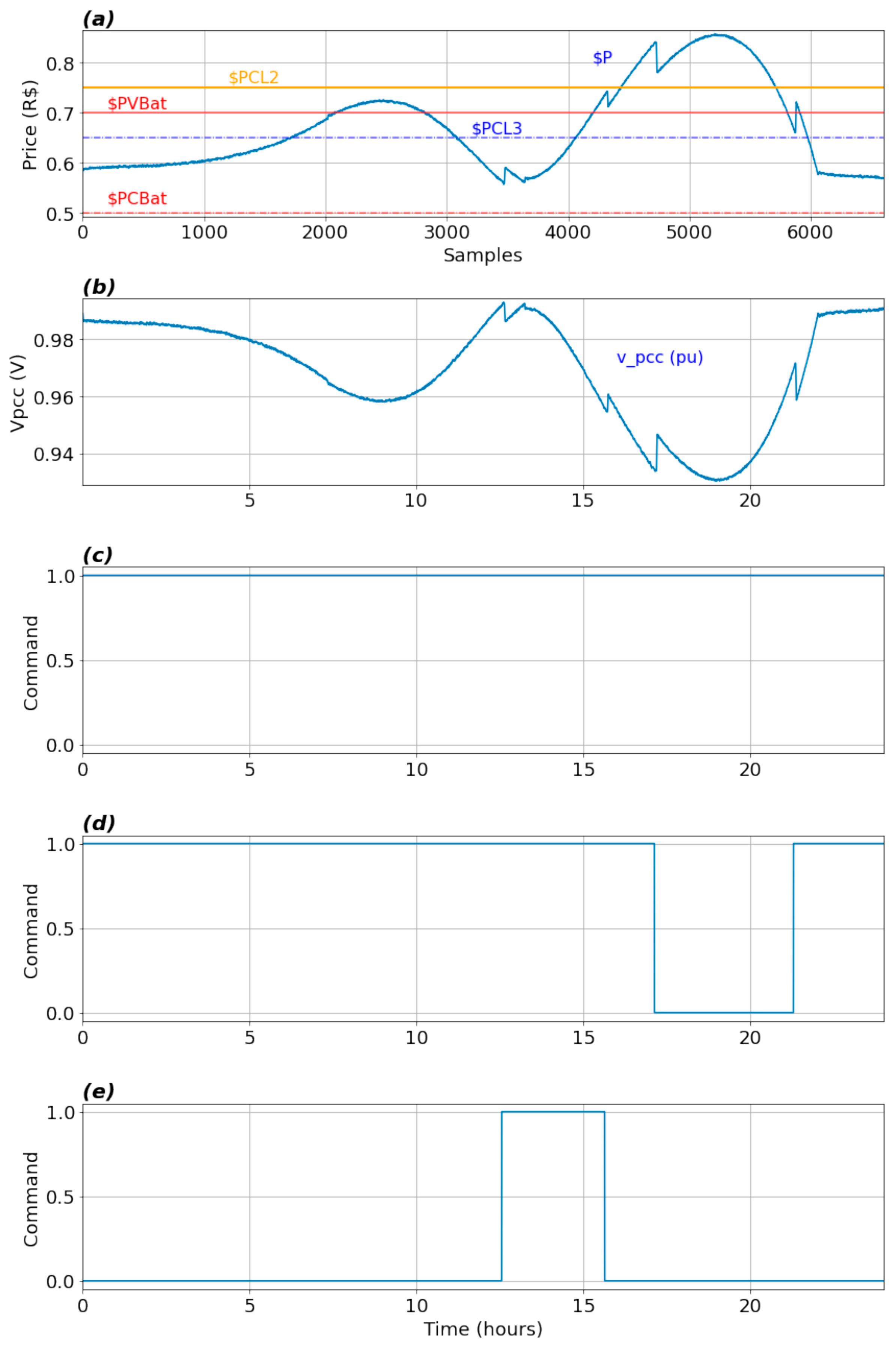
The first graphic time axis is in number of samples, for a matter of experiment time evidence, with a period between them of less than half of a second, while the others are presented in hours. The net power in the bus determines the voltage level, as shown in Figure 24b, and the power sale and purchase prices in (a). In the graphics, stands for the price of energy, stands for the sale price for the battery bank, stands for the purchase price, stands for the load 2 purchase price and stands for the load 3 purchase price. So, when the price goes above or below , the battery bank connects to the MR and, respectively, buys the surplus of energy or sells what is lacking. Its functioning as a load or a source occurs naturally, since the bus voltage (Vpcc) is above the reference voltage (1 pu) at purchase, which makes energy flow from the bus to the bank, and the opposite in the sale. The droop power references act by imposing how much power (active/reactive) must be transferred.
The command signals (c–e) sent from the controller to the switches can also be observed, enabling the connection of the units to the bus. These graphs show the status of each command, whether connected or not, considering the price and the established threshold of purchase and sale. The connection does not take place exactly when the price limit is exceeded, because there are hysteresis bands that delay the connection/disconnection. The connection command for the battery bank is the same for both sales and purchases, which is possible because those are different situations. In the case of selling, the bank receives a signal to connect, and the bus voltage is lower than that of the bank’s converter. The opposite takes place in the case of purchasing.
3.2. Second Scenario
The second scenario presents, in Figure 25a, the main load reactive power consumption curve in high level, and the photovoltaic generator in low active power production (f). The main grid provides (b) only what is lacking to complete the consumption from the loads, both active and reactive power. The battery bank can supply (c) what is lacking for all the loads or absorb the surplus. The secondary loads (e) remain connected most of the time, considering the active power lower price commercialization.
The reactive energy price, shown in Figure 26a, slightly increases because of the reactive power scarcity: (b) shows the bus angle, (c) shows the active energy price, and the bus voltage is shown in (d). The sale of battery reactive energy in the first connection occurs because there is no selective control of reactive power supply. As the connection to supply the active power occurred, the reactive power was supplied simultaneously, but it should not necessarily be so. If there is no interest in supplying reactive power, it would be enough to act in the control of the reactive load dispatch.
3.3. Third Scenario
The MG is islanded, as Figure 27b shows. The renewable energy source is in low level (f), so is the main load (a), the bus active power is scarce and the storage bank (c) operates connected all the time. The power consumed by the main load was almost entirely supplied by the storage bank (d), consuming almost all the reserves. Due to the scarcity, the medium priority load turns off for a certain time, which did not happen in the previous scenarios, and the lower priority load remains off during almost the entire experiment.
The bus active power in this scenario determines the voltage level, as Figure 28b shows, and the energy prices (a) for sale and purchase, as well as the control signals, are sent (c–e) from the controller to the connection switches.
4. Conclusions
This work presents an AC MG power management approach based on microeconomics theories for market equilibrium, enabling automatic power management for distributed sources and loads through AC bus signaling, which is valid for all types of converters, grid supporting, grid feeding and grid forming, in a decentralized control system. The results demonstrate that the strategy meets the control requirements established by the most recent research papers, easily managing the balance between demanded and supplied power in an MG, sharing the supply among sources, controlling the bus voltage and frequency in a more decentralized manner of managing the system.
The approach establishes the balance between demand and supply of active power in an MG using the AC bus voltage amplitude as a price signal, emulating the functioning of the free market, integrating technical and economic issues and using this same principle to control the reactive power by varying the angle (connected mode) and frequency (islanded mode). This strategy has some advantages, such as the use of an easy-to-understand approach, based on mature industry knowledge and in line with the latest works presented by the scientific community. A key element of the control design was the operation of the MG sources without the need for a communication network between the MG components, since the low-bandwidth communication function could be performed in many ways. Therefore, the controller of each source must be able to respond effectively to changes in the system without requiring data from other sources or locations. In addition, there would be the possibility of the MG optimizing energy/costs, the bus voltage profile, as well as other desirable characteristics, such as a distributed control, an easy connection, few rules for participants (Plug and Play), the use of ACBS and droop control, simplicity of principles and operation, and a low operating cost.
The strategy presented contributes to the hierarchical control structure, with one more option of a decentralized control implementation for the primary and secondary levels. It reduces model complexity, increasing the system robustness, giving more operational flexibility, managing the active demand, collaborating to a better integration between the MG and the storage systems and providing scalability for this solution.
The results confirm that a proper MG operation is possible even in different operating scenarios. The conditions considered for the MG operation in this work were more severe than those normally found in an ordinary situation. So, the critical points could be learned for the operation and the development of suitable solutions for this technique. The follow-up works should consider a real MG implementation, exploring more possibilities for control at the secondary and tertiary levels, considering tools for system optimization, issues of protection/security, stability, harmonics and synchronization.
Author Contributions
Conceptualization, M.M., L.M., L.V.B. and L.F.R.P.; methodology, M.M. and L.F.R.P.; software, T.D.C.B. and L.F.R.P.; validation, M.M., L.M., L.V.B. and L.F.R.P.; formal analysis, M.M., L.M., L.V.B., T.D.C.B. and L.F.R.P.; investigation, M.M. and L.F.R.P.; resources, M.M., L.M.; data curation, M.M. and L.F.R.P.; writing—original draft preparation, M.M. and L.F.R.P.; writing—review and editing, M.M., L.M., L.V.B., T.D.C.B. and L.F.R.P.; visualization, M.M., L.M., L.V.B., T.D.C.B. and L.F.R.P.; supervision, M.M. and L.M.; project administration, M.M.; funding acquisition, M.M. and L.M. All authors have read and agreed to the published version of the manuscript.
Funding
This research was funded by Conselho Nacional de Desenvolvimento Cientifico e Tecnologico (CNPq) grant number 465640/2014-1, Coordenacao de Aperfeicoamento de Pessoal de Nivel Superior (CAPES) grant number 23038.000776/2017-54, Fundacao de Amparo a Pesquisa do Estado do Rio Grande do Sul (FAPERGS), grant number 17/2551-0000517-1; Fundacao de Amparo a Pesquisa e Inovacao do Estado de Santa Catarina (FAPESC), grant number 2021TR893, and Universidade do Estado de Santa Catarina (UDESC).
Institutional Review Board Statement
Not applicable for studies not involving humans or animals.
Informed Consent Statement
Not applicable for studies not involving humans or animals.
Data Availability Statement
Not applicable.
Acknowledgments
This work was developed with the support of Programa Nacional de Cooperacao Academica da Coordenacao de Aperfeicoamento de Pessoal de Nivel Superior—CAPES/Brazil. This research was funded by Conselho Nacional de Desenvolvimento Cientifico e Tecnologico (CNPq); Coordenacao de aperfeicoamento de Pessoal de Nivel Superior (CAPES); Fundacao de Amparo a Pesquisa do Estado do Rio Grande do Sul (FAPERGS); Fundacao de Amparo a Pesquisa e Inovacao do Estado de Santa Catarina (FAPESC) and Universidade do Estado de Santa Catarina (UDESC).
Conflicts of Interest
The funders had no role in the design of the study; in the collection, analyses, or interpretation of data; in the writing of the manuscript, or in the decision to publish the results.
Abbreviations
The following abbreviations are used in this manuscript:
| MG | Microgrid |
| AC | Alternating Current |
| DC | Direct Current |
| PMS | Power Management System |
| EES | Energy Storage System |
| DBS | Direct Current Bus Signaling |
| ACBS | Alternating Current Bus Signaling |
| TOU | Time of Use |
| DR | Demand Response |
| PCC | Point of Common Coupling |
| SOC | State of Charge |
| SOH | State of Health |
References
- Tahim, A.P.N. Controle de MR de Distribuição de Energia Elétrica em CC. Master’s Thesis, UFSC, Florianópolis, Brazil, 2015. [Google Scholar]
- Basak, P.; Chowdhury, S.; HalderneeDey, S.; Chowdhury, S.P. A literature Review on Integration of Distributed Energy Resources in the Perspective of Control, Protection and Stability of Microgrid. Proc. Renew. Sustain. Energy Rev. 2012, 16, 5545–5556. [Google Scholar] [CrossRef]
- Hartono, B.S.; Budiyanto, Y.; Setiabudy, R. Review of Microgrid Technology. Proc. Qual. Res. 2013, 2013, 127–132. [Google Scholar]
- Nikos, D.H. Trends in Microgrid Control. IEEE Trans. Smart Grid 2012, 5, 1905–1919. [Google Scholar]
- Planas, E.; Gil-de-Muro, A.; Andreu, K.I.; Alegría, I.M. General aspects, hierarchical controls and droop methods in microgrids: A review. Proc. Renew. Sustain. Energy Rev. 2012, 17, 147–159. [Google Scholar] [CrossRef]
- Jiang, Z.; Dougal, R. Hierarchical Microgrid Paradigm for Integration of Distributed Energy Resources. In Proceedings of the 2008 IEEE Power and Energy Society General Meeting, Pittsburgh, PA, USA, 20–24 July 2008; pp. 1–8. [Google Scholar]
- Correa, E.P. Estudo de um Modelo de Ordem Reduzida para a Análise da Estabilidade de Microrredes CA. Master’s Thesis, UDESC, Joinville, Brazil, 2018. [Google Scholar]
- Vandoorn, T.L.; Vasquez, J.C.; De Kooning, J.; Guerrero, J.M.; Vandevelde, L. Microgrids: Hierarchical control and an overview of the control and reserve management strategies. IEEE Ind. Electron. Mag. 2013, 7, 42–55. [Google Scholar] [CrossRef] [Green Version]
- Biglarahmadi, M.; Ketabi, A.; Baghaee, H.R.; Guerrero, J.M. Integrated Nonlinear Hierarchical Control and Management of Hybrid AC/DC Microgrids. IEEE Syst. J. 2021, 16, 902–913. [Google Scholar] [CrossRef]
- Vasquez, J.C.; Guerrero, J.M.; Miret, J.; Castilha, M.; Vicuna, L.G. Hierarchical Control of Inteligent Microgrids. Proc. IEEE Ind. Electron. Mag. 2010, 12, 23–29. [Google Scholar] [CrossRef]
- Zhao, E.; Liu, E.; Li, L.; Han, Y.; Yang, P.; Wang, C. Hierarchical Control Strategy Based on Droop Coefficient Calibration and Bus Voltage Compensation for DC Microgrid Cluster. In Proceedings of the IEEE 2nd China International Youth Conference on Electrical Engineering, Chengdu, China, 15–17 December 2021. [Google Scholar]
- Guerrero, J.M.; Vasquez, J.C.; Matas, J.; Vicuna, L.G.; Castilha, M. Hierarchical Control of Droop-Controlled AC and DC Microgrids—A General Approach Toward Standardization. In Proceedings of the IEEE Transactions on Industrial Electronics, Chengdu, China, 15–17 December 2011; Volume 58, p. 1. [Google Scholar]
- Feng, F.; Zhang, P. Enhanced Microgrid Power Flow Incorporating Hierarchical Control. IEEE Trans. Power Syst. 2020, 35, 3. [Google Scholar] [CrossRef] [Green Version]
- Rocabert, J.; Luna, A.; Blaabjerg, F.; Rodriguez, P. Control of Power Converters in AC Microgrids. Proc. IEEE Trans. Power Electron. 2012, 27, 4734–4749. [Google Scholar] [CrossRef]
- Li, Z.; Cheng, Z.; Si, J.; Li, S. Distributed Event-Triggered Hierarchical Control to Improve Economic Operation of Hybrid AC/DC Microgrids. IEEE Trans. Power Syst. 2021, 12, 1. [Google Scholar] [CrossRef]
- Bidram, A.; Davoudi, A. Hierarchical Structure of Microgrids Control System. Proc. IEEE Trans. Smart Grid 2012, 3, 1963–1976. [Google Scholar] [CrossRef]
- Molist, C.C.; Bazmohammadi, N.; Vasquez, J.C.; Dussap, C.-G.; Guerrero, J.M.A. Hierarchical Control of Space Closed Ecosystems—Expanding Microgrid Concepts to Bioastronautics. IEEE Ind. Electron. Mag. 2020, 15, 2. [Google Scholar]
- Mohammed, A.; Mohammed, S.; Refaat, S.; Bayhan, S.; Abu-Rub, H. AC Microgrid Control and Management Strategies: Evaluation and Review. Proc. IEEE Power Electron. Mag. 2019, 6, 2. [Google Scholar] [CrossRef]
- Morstyn, T.; Hredzak, B.; Agelidis, V. Control Strategies for Microgrids with Distributed Energy Storage Systems: An Overview. Proc. IEEE Trans. Smart Grid 2018, 9, 3652–3666. [Google Scholar] [CrossRef] [Green Version]
- Singh, J.; Singh, S.P.; Verma, K.S.; Iqbal, A.; Kumar, B. Recent control techniques and management of AC microgrids: A critical review on issues, strategies, and future trends. Proc. Int. Trans. Electr. Energy Syst. Conf. 2021, 31, e13035. [Google Scholar] [CrossRef]
- Jackson, J.; Mwasilu, F.; Lee, J.; WooJung, J. AC-microgrids versus DC-microgrids with distributed energy resources: A review. Proc. Renew. Sustain. Energy Rev. 2013, 24, 387–405. [Google Scholar]
- Quintana, P.J.; Garcia, J.; Guerrero, J.M.; Dragicevic, T.; Vasquez, J.C. Control of single-phase islanded PV/battery street light cluster based on Power-Line Signaling. In Proceedings of the 2013 International Conference on New Concepts in Smart Cities: Fostering Public and Private Alliances (SmartMILE), Gijon, Spain, 11–13 December 2013; pp. 1–6. [Google Scholar]
- Shafiee, Q.; Dragicevic, T.; Andrade, F.; Vasquez, J.C.; Guerrero, J.M. Distributed Consensus-Based Control of Multiple DC-Microgrids Clusters. In Proceedings of the 40th Annual Conference of IEEE Industrial Electronics Society, Sheraton Hotel Dallas, Dallas, TX, USA, 29 October–1 November 2014. [Google Scholar]
- Glavic, M. Agents and Multi-Agent Systems: A Short Introduction for Power Engineers; University of Liege Electrical Engineering and Computer Science Department: Liege, Belgium, 2006; pp. 1–21. [Google Scholar]
- Shafiee, Q.; Guerrero, J.M.; Vasquez, J.C. Distributed Secondary Control for Islanded Microgrids—A Novel Approach. Proc. IEEE Trans. Power Electron. 2014, 29, 1018–1031. [Google Scholar] [CrossRef] [Green Version]
- Araujo, L.S.; Alonso, A.M.S.; Brandao, D.I. Decentralized Control of Voltage- and Current-Controlled Converters Based on AC Bus Signaling for Autonomous Microgrids. Proc. IEEE Access 2020, 8, 202075–202089. [Google Scholar] [CrossRef]
- Schönberger, J.; Duke, R.; Round, S. DC-Bus Signaling: A Distributed Control Strategy for a Hybrid Renewable Nanogrid. Proc. IEEE Trans. Ind. Electron. 2006, 53, 1453–1460. [Google Scholar] [CrossRef]
- Guerrero, J.M.; Chandorkar, M.; Lee, T.L.; Loh, P.C. Advanced Control Architectures for Intelligent Microgrids Part I and II: Decentralized and Hierarchical Control. Proc. IEEE Trans. Ind. Electron. 2013, 60, 1263–1270. [Google Scholar] [CrossRef] [Green Version]
- Sun, K.; Zhang, L.; Xing, Y.; Guerrero, J.M. A Distributed Control Strategy Based on DC Bus Signaling for Modular Photovoltaic Generation Systems With Battery Energy Storage. Proc. IEEE Trans. Power Electron. 2014, 61, 3313–3326. [Google Scholar]
- Bryan, J.; Duke, R.; Round, S. Decentralized Generator Scheduling in a Nanogrid Using DC Bus Signaling. In Proceedings of the IEEE Power Engineering Society General Meeting, Denver, CO, USA, 6–10 June 2004. [Google Scholar]
- Schiller, B. The Micro Economy Today, 11th ed.; McGraw-Hill: New York, NY, USA, 2008. [Google Scholar]
- Sharifi, R.; Anvari-Moghaddam, A.; Fathi, S.H.; Guerrero, J.M.; Vahidinasab, V. Dynamic Pricing: An Efficient Solution for True Demand Response Enabling. Proc. J. Renew. Sustain. Energy 2017, 10, 065502. [Google Scholar] [CrossRef] [Green Version]
- Bellinaso, L.V.; Schwertner, C.D.; Michels, L. Price-based power management of off-grid photovoltaic systems with centralised dc bus. Proc. IET Renew. Power Gener. 2016, 10, 1132–1139. [Google Scholar] [CrossRef]
- Bellinaso, L.V.; Edivan, L.C.; Cardoso, R.; Michels, L. Price-Response Matrices Design Methodology for Electrical Energy Management Systems Based on DC Bus Signalling. Proc. Energies J. 2021, 14, 1787. [Google Scholar] [CrossRef]
- Zimann, F.J. Sistema de Controle de Potência Ativa e Reativa para a Regulação de Tensão em Redes de Distribuição de Baixa Tensão. Master’s Thesis, UDESC, Joinville, Brazil, 2016. [Google Scholar]
- de Azevedo, G.M.S. Controle e Operação de Conversores em Microrredes. Ph.D Thesis, UFPe, Pernanbuco, Brazil, 2011. [Google Scholar]
- Maryama, V. Análise de Estratégias de Divisão de Carga Baseadas em Droop para Microrredes. Master’s Thesis, UFSC, Florianópolis, Brazil, 2016. [Google Scholar]
- AgêNcia Nacional de Energia EléTrica. Available online: https://www.aneel.gov.br/editais-de-geracao (accessed on 15 February 2022).
Figure 1.
(a) Price versus Supply. (b) Price versus Demand.

Figure 2.
Supply versus demand curve.
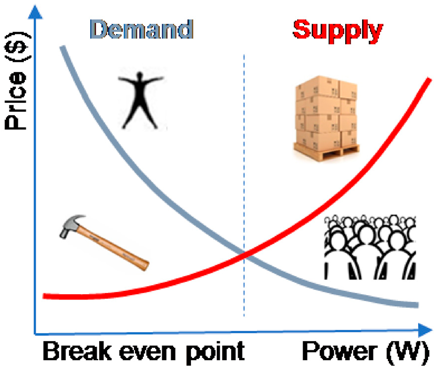
Figure 3.
Operating loads cycles.
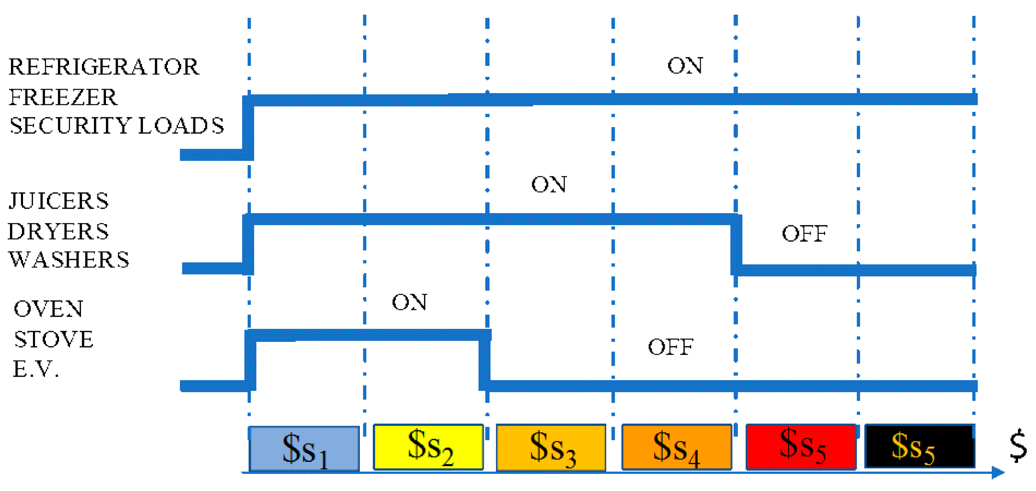
Figure 4.
Operating load cycles.
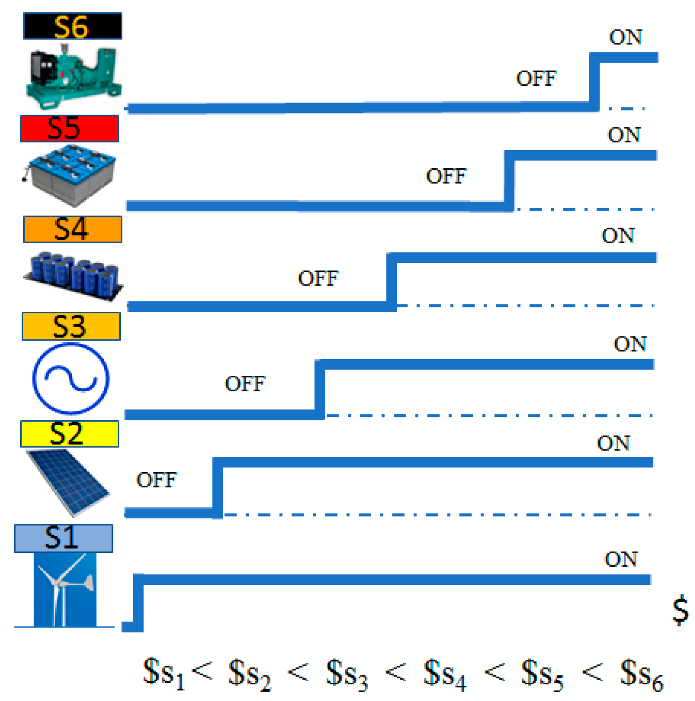
Figure 5.
Grid/MG connection model. (a) Equivalent circuit. (b) Phasor diagram.
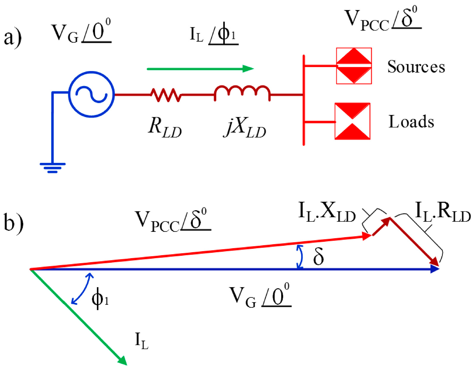
Figure 6.
Model for Islanded Operation. (a) GSC current source. (b) GSC voltage source. (c) Droop active power (V × P). (d) Droop reactive power (f × Q).
Figure 6.
Model for Islanded Operation. (a) GSC current source. (b) GSC voltage source. (c) Droop active power (V × P). (d) Droop reactive power (f × Q).
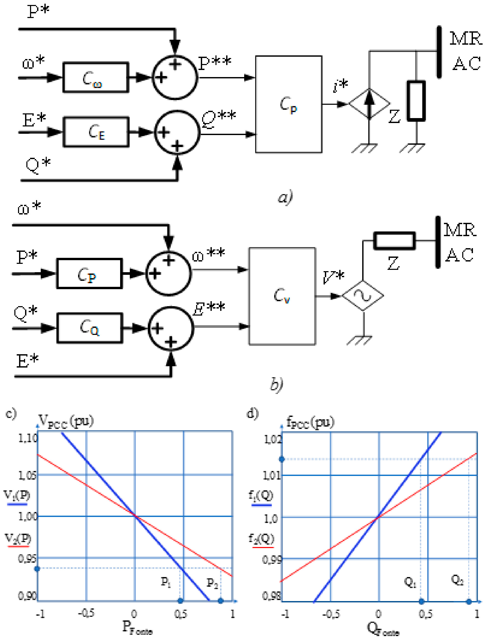
Figure 7.
Relationship between power (P, Q) and measurements at the PCC. (a) Relationship between bus active power and voltage. (b) Relationship between bus reactive power and angle. (c) Relationship between bus reactive power and frequency.
Figure 7.
Relationship between power (P, Q) and measurements at the PCC. (a) Relationship between bus active power and voltage. (b) Relationship between bus reactive power and angle. (c) Relationship between bus reactive power and frequency.

Figure 8.
Relationship between parameters at the bus and power price. (a) Relationship between bus voltage and price. (b) Relationship between angle and price. (c) Relationship between bus frequency and price.
Figure 8.
Relationship between parameters at the bus and power price. (a) Relationship between bus voltage and price. (b) Relationship between angle and price. (c) Relationship between bus frequency and price.
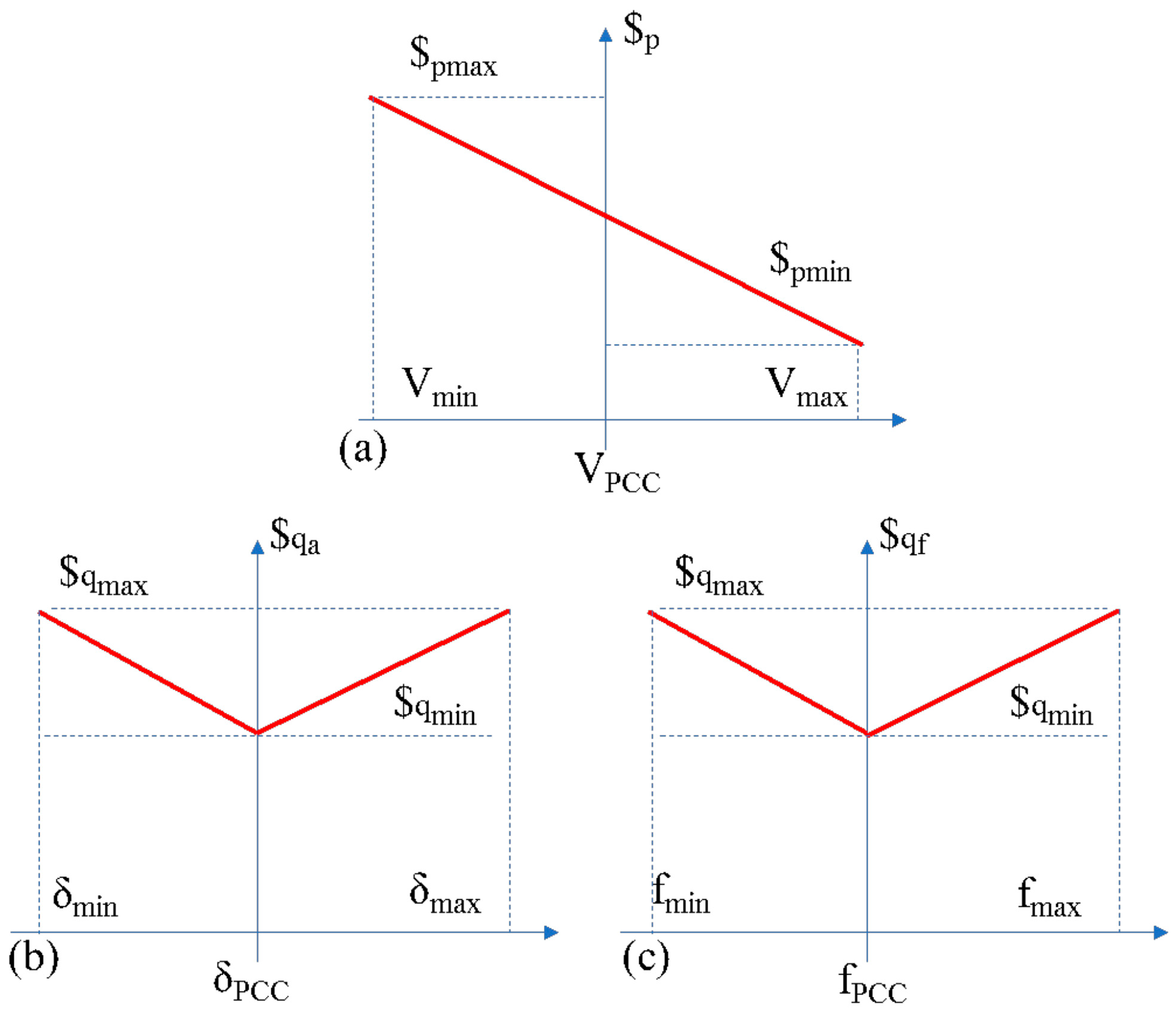
Figure 9.
Relationship between bus measurements and prices. (a) Vertical offset. (b) Different slope.
Figure 9.
Relationship between bus measurements and prices. (a) Vertical offset. (b) Different slope.

Figure 10.
An autonomous decentralized AC MG general structure.
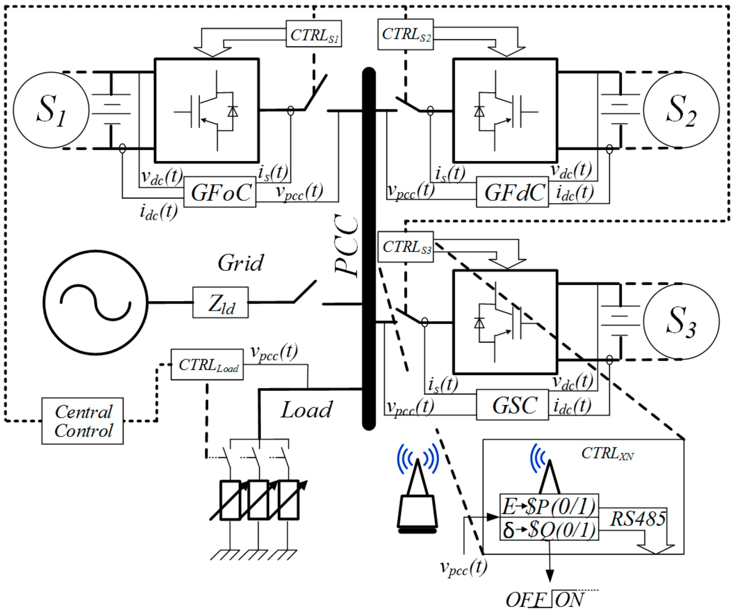
Figure 11.
Implemented DSC code flowchart.
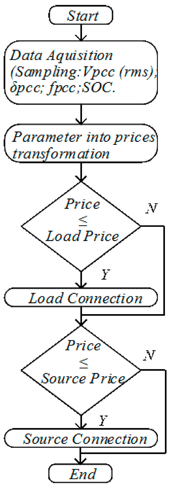
Figure 12.
Price evolution, connection and chattering.
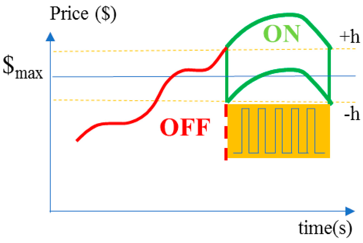
Figure 13.
MG SCADA user interface.

Figure 14.
Main load in HIL experiment block.

Figure 15.
Low-priority loads experiment block.

Figure 16.
Main grid experiment block.
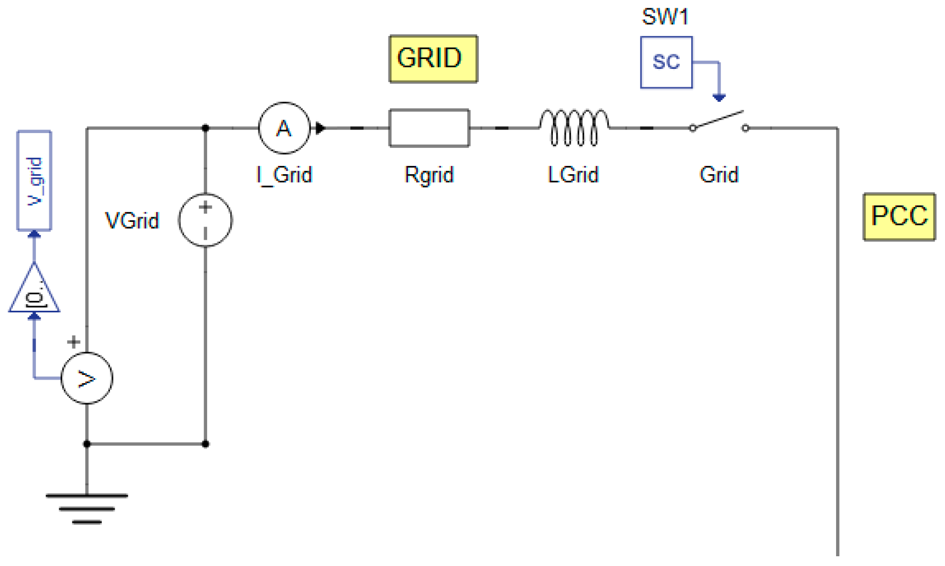
Figure 17.
PV generator experiment blocks.

Figure 18.
Battery bank experiment blocks.
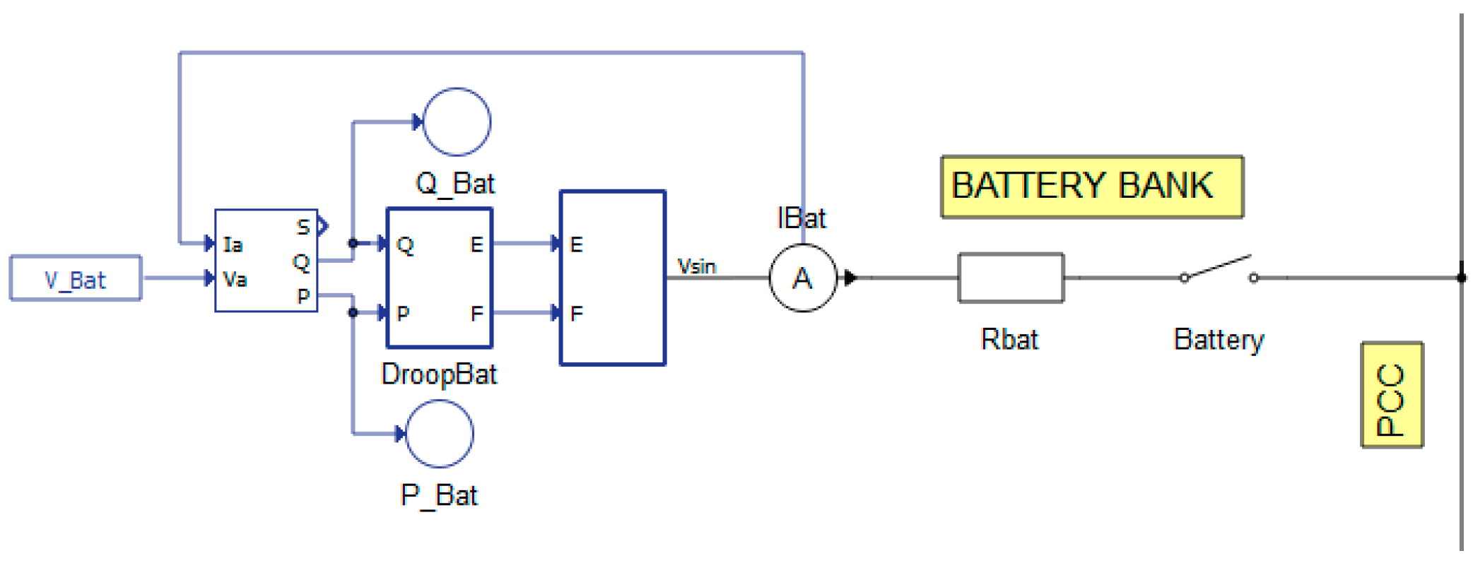
Figure 19.
Droop control blocks.

Figure 20.
Converter experiment blocks.
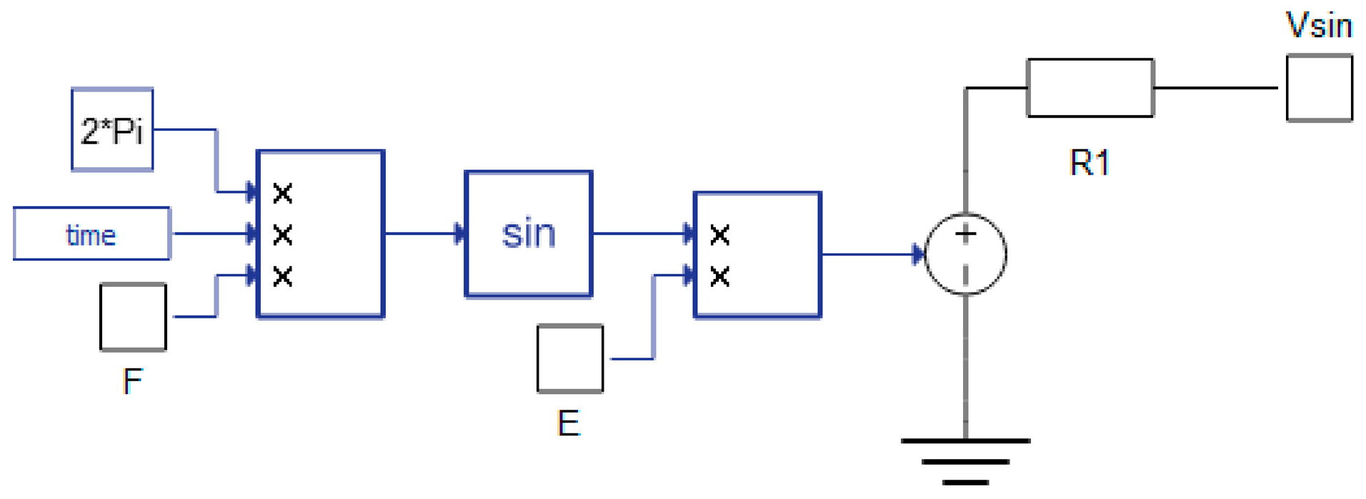
Figure 21.
Specified purchase and sale prices for each MG unit.

Figure 22.
HIL simulator, with interface board and attached micro controller.

Figure 23.
MG operating in connected mode with bus abundance of active power. Power values: (a) Main load active power; (b) Main grid active power; (c) Battery bank active power; (d) Battery storage level; (e) Load 2 and 3 active power; (f) Photovoltaic active power.
Figure 23.
MG operating in connected mode with bus abundance of active power. Power values: (a) Main load active power; (b) Main grid active power; (c) Battery bank active power; (d) Battery storage level; (e) Load 2 and 3 active power; (f) Photovoltaic active power.
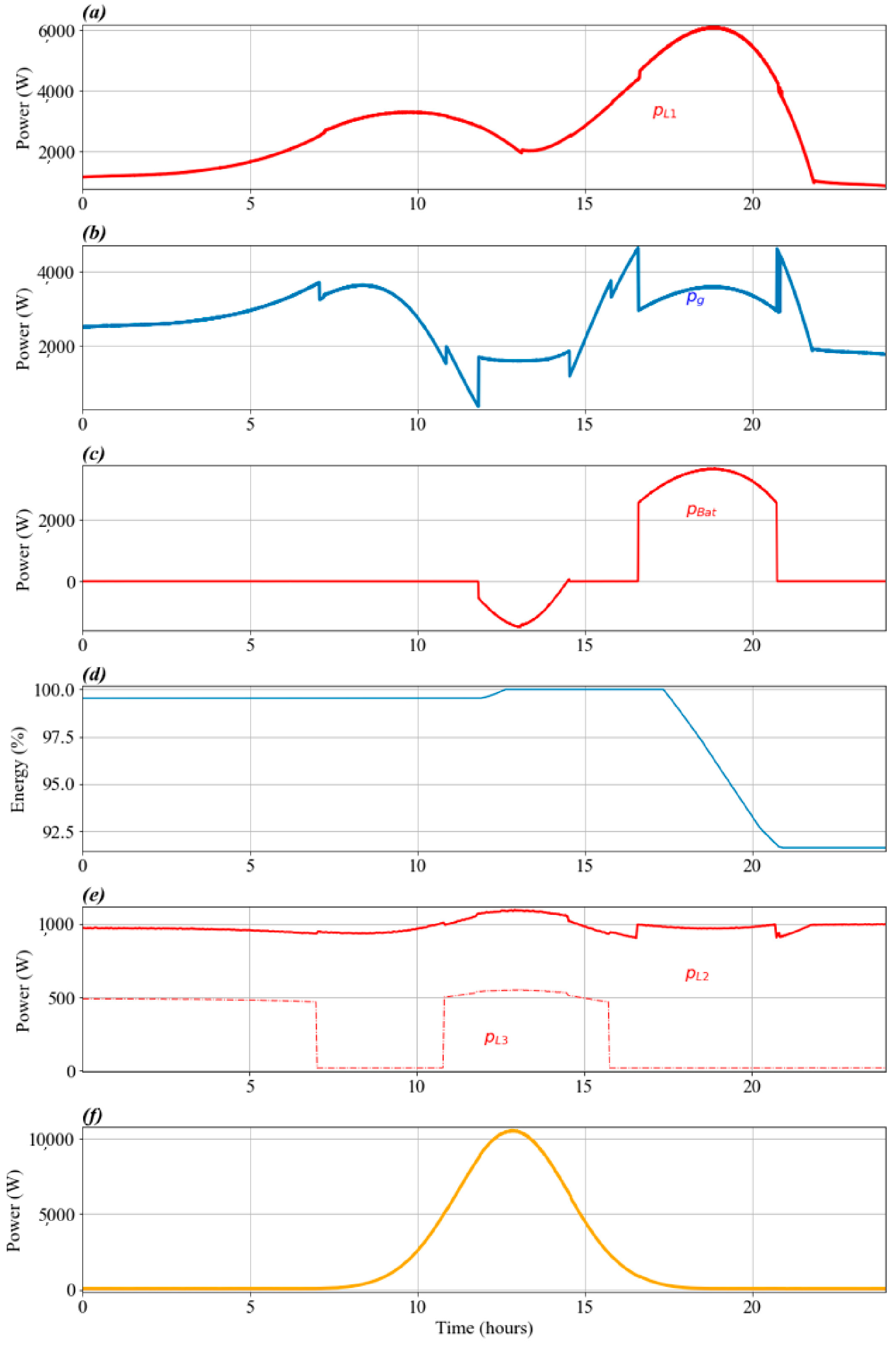
Figure 24.
MG operating in connected mode with bus abundance of active power. Commands: (a) Energy price; (b) Bus voltage; (c) Battery bank command; (d) Load 2 command; (e) Load 3 command.
Figure 24.
MG operating in connected mode with bus abundance of active power. Commands: (a) Energy price; (b) Bus voltage; (c) Battery bank command; (d) Load 2 command; (e) Load 3 command.

Figure 25.
MG operating in connected mode with reactive power consumption. Power values: (a) Main load reactive power; (b) Main grid power; (c) Battery bank power; (d) Battery storage level; (e) Load 2 and 3 active power; (f) Photovoltaic active power.
Figure 25.
MG operating in connected mode with reactive power consumption. Power values: (a) Main load reactive power; (b) Main grid power; (c) Battery bank power; (d) Battery storage level; (e) Load 2 and 3 active power; (f) Photovoltaic active power.
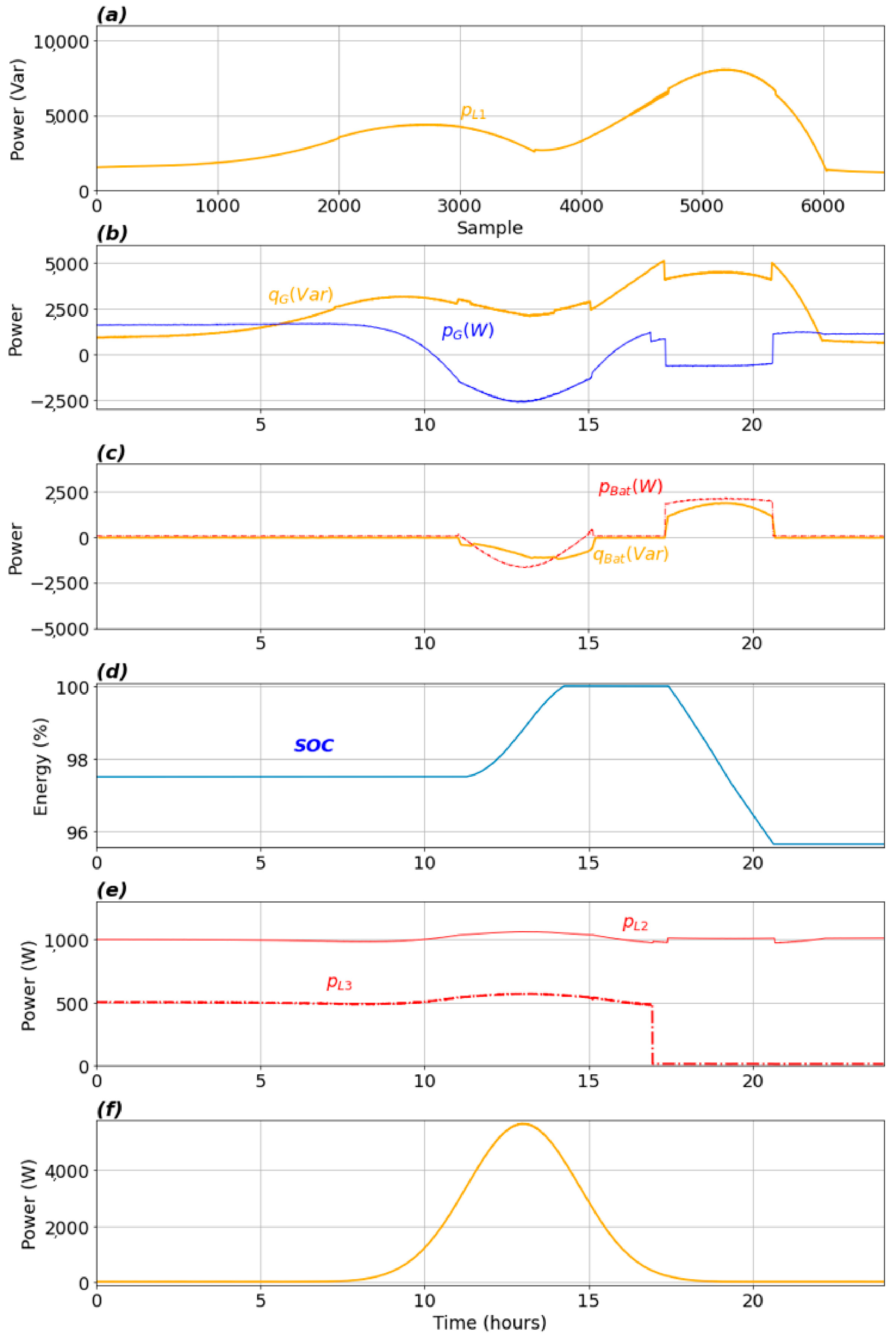
Figure 26.
MG operating in connected mode with reactive power consumption. Commands: (a) Reactive energy price; (b) Bus angle; (c) Active energy price; (d) Bus voltage; (e) Battery bank command; (f) Load e and 3 Command.
Figure 26.
MG operating in connected mode with reactive power consumption. Commands: (a) Reactive energy price; (b) Bus angle; (c) Active energy price; (d) Bus voltage; (e) Battery bank command; (f) Load e and 3 Command.
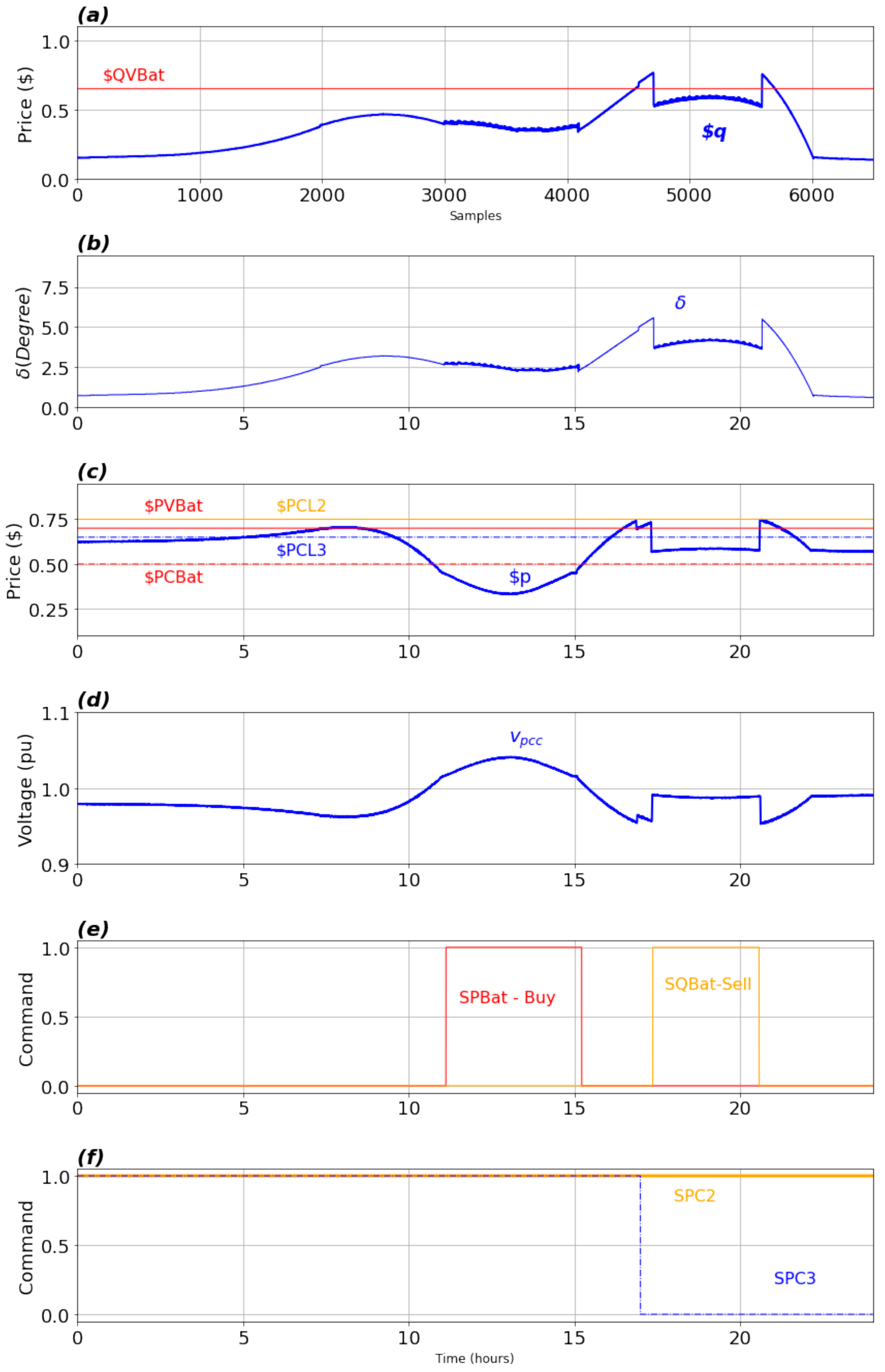
Figure 27.
MG operating in islanded mode with active power consumption. Power values: (a) Main load active power; (b) Main grid power; (c) Battery bank active power; (d) Battery storage level; (e) Load 2 and 3 active power; (f) Photovoltaic active power.
Figure 27.
MG operating in islanded mode with active power consumption. Power values: (a) Main load active power; (b) Main grid power; (c) Battery bank active power; (d) Battery storage level; (e) Load 2 and 3 active power; (f) Photovoltaic active power.
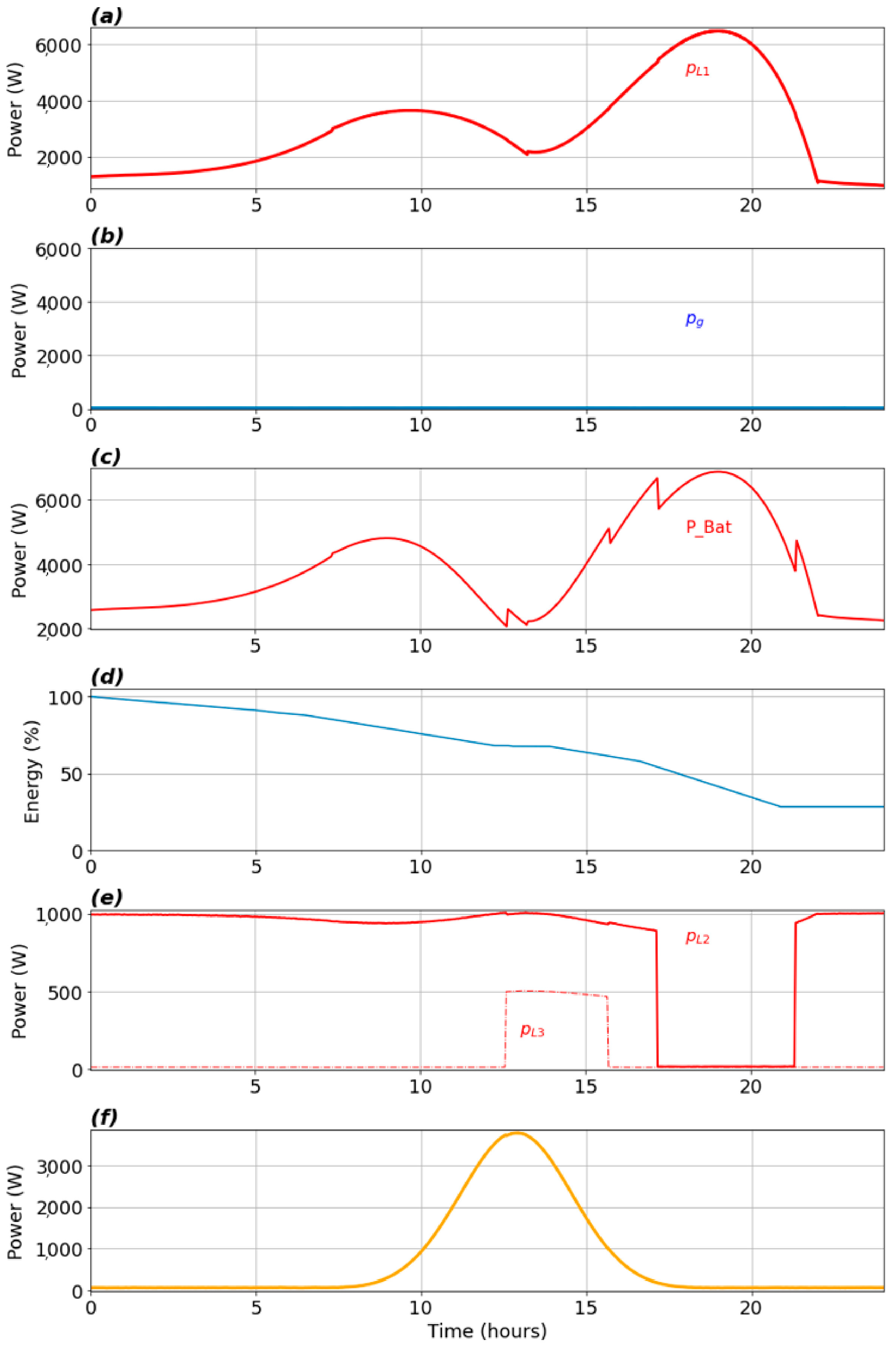
Figure 28.
MG operating in islanded mode with active power consumption. Commands: (a) Active energy price; (b) Bus voltage; (c) Battery bank command; (d) Load 2 command; (e) Load 3 command.
Figure 28.
MG operating in islanded mode with active power consumption. Commands: (a) Active energy price; (b) Bus voltage; (c) Battery bank command; (d) Load 2 command; (e) Load 3 command.

Table 1.
The MG parameters.
| Description | Values |
|---|---|
| Load 1/Rated Grid Power | = = 12 kVA |
| Load 2/3 Rated Power | = 1 kW/0.5 kW |
| Rated Battery Power | = 10 kVA |
| Rated PV Power | = 10 kW |
| Rated AC-Phase rms Voltage | = 220 V |
| Allowed MG Voltage Range | VCA = ±10% |
| Rated Grid Frequency | = 60 Hz |
| Allowed MG Frequency Range | F = ±0.02 pu |
| Distribution Line Inductance | = 858.9 F |
| Distribution Line Reactance | = 0.32 |
| Distribution Line Resistance | = 0.77 |
| Distribution Line Impedance | = 0.84 |
Publisher’s Note: MDPI stays neutral with regard to jurisdictional claims in published maps and institutional affiliations. |
© 2022 by the authors. Licensee MDPI, Basel, Switzerland. This article is an open access article distributed under the terms and conditions of the Creative Commons Attribution (CC BY) license (https://creativecommons.org/licenses/by/4.0/).
Share and Cite
MDPI and ACS Style
Pinto, L.F.R.; Busarello, T.D.C.; Bellinaso, L.V.; Michels, L.; Mezaroba, M. Contributions to Power Management in AC Microgrids Based on Concepts of Microeconomics Theory. Energies 2022, 15, 3890. https://doi.org/10.3390/en15113890
AMA Style
Pinto LFR, Busarello TDC, Bellinaso LV, Michels L, Mezaroba M. Contributions to Power Management in AC Microgrids Based on Concepts of Microeconomics Theory. Energies. 2022; 15(11):3890. https://doi.org/10.3390/en15113890
Chicago/Turabian StylePinto, Luís F. R., Tiago D. C. Busarello, Lucas V. Bellinaso, Leandro Michels, and Marcello Mezaroba. 2022. "Contributions to Power Management in AC Microgrids Based on Concepts of Microeconomics Theory" Energies 15, no. 11: 3890. https://doi.org/10.3390/en15113890
Note that from the first issue of 2016, this journal uses article numbers instead of page numbers. See further details here.