
Implementation and Critical Analysis of the Active Phase Jump with Positive Feedback Anti-Islanding Algorithm


Faculty of Electrical Engineering, Federal University of Uberlandia, Uberlandia 38400-902, Brazil
*
Author to whom correspondence should be addressed.
Energies 2022, 15(13), 4609; https://doi.org/10.3390/en15134609
Submission received: 23 May 2022
/
Revised: 16 June 2022
/
Accepted: 16 June 2022
/
Published: 23 June 2022
(This article belongs to the Special Issue Control of Distributed Power Electronic Converters in Smart Energy Systems)
Abstract
:The protection against the unintentional islanding of Grid-Tied inverters is an important electrical security issue addressed by the main Standards. This concern is justified in face of the fact that unintentional islanding can lead to abrupt variations of voltage and frequency, electrical damages, professional accidents, power quality degradation, and out-of-phase reclosure. In response to the islanding concern, the literature has proposed several Anti-Islanding Protection (AIP) schemes that can be divided in passive and active methods. Many of the active AIP is based on the insertion of some disturbance in the inverter current in order to deviate the frequency out of the allowed thresholds, tripping the inverter internal disconnection system. Thus, the main objective of this paper is to analyze the performance of the Active Phase Jump with Positive Feedback (APJPF) algorithm compared to other well-known frequency drift-based solutions. More than that, this work covers the Non-Detection Zone (NDZ) problem, analyzing its main mapping methodologies and the normative requirements, exposing the minimum normative recommendations a given AIP must reach to be considered functional. The last contributions of this paper are the proposal of a parametrization criterion for the Active Frequency Drift with Pulsating Chopping Factor (AFDPCF) and for the APJPF.
1. Introduction
The growing penetration of Grid-Tie Photovoltaics Systems (GTPS) must obey to energy quality criteria and security considerations in order to guarantee the safeness of users and operators. The Standards are the documents that determine the voltage, frequency, power factor, and the Total Harmonic Distortion of Voltage (THDv) and Current (THDi) requirements in which the inverter must operate to avoid power quality degradation. Beyond that, the Standards regulate the minimum safety goals an electrical device must reach to be allowed to operate in parallel with the main utility grid. Among the several protections addressed by [1,2,3,4], it is possible to cite reverse power flow, frequency and voltage deviations, shortcuts, flickers, and islanding.
The islanding phenomenon occurs when a portion of the electrical system that receives power, concomitantly, from a GTPS and the utility grid, remains energized after the grid interruption [2]. It is necessary to state that this contingence can be intentional or unintentional. While the intentional islanding is a powerful tool to ensure power to isolated areas, unintentional islanding has no positive bias and provokes the growing of the THDv rates, electrical accidents, and out-of-phase reclosure [5].
In this way, a massive number of Anti-Islanding Protection (AIP) strategies were proposed in order to guarantee the fast and reliable inverter shutdown after the grid interruption. It is necessary, therefore, to categorize them according to its functioning principle and essential characteristics. In this context, AIP strategies can be divided in passive and active solutions [6].
The passive methods are defined by the pure monitoring of an electrical variable of operation and the inverter shutdown occurs after the detection of some abnormality during a pre-set time interval [7]. The main examples of passive AIP solutions are: Over-Under Voltage (OUV) or Frequency (OUF) [8] detection, Phase Jump Detection [9], THDv Detection [10], Rate of Change of Frequency (ROCOF) [11], or Voltage (ROCOV) [12]. The main advantages of the passive strategies lie in the fact that they are not intrusive in relation to the power quality, since they do not insert any kind of disturbance during the inverter operation [13]. However, passive AIP loses reliability when there is a balance between the power produced by the GTPS and the power demanded by the islanded loads [14].
In order to improve AIP techniques, guaranteeing the detection of the grid interruption, even in conditions of balance between the energy generated by the photovoltaic array and the energy required by the local loads, active techniques were proposed. In addition to the monitoring of some electrical variable behavior, active AIP inserts small perturbations to destabilize the inverter after the islanding occurrence [15]. Although its implementation is inherently linked to the power quality degradation, its adoption is justified by the mitigation of the Non-Detection Zone (NDZ) problem, which will be addressed in the next sections [16]. Among the major representative of this class, it is possible to highlight Active Frequency Drift (AFD) [17], Sandia Frequency Shift (SFS) [18], Slip Mode Shift (SMS) [19], and Active Frequency Drift with Pulsating Chopping Factor (AFDPCF) [20].
It is necessary to cite that the first active AIP was the AFD, characterized by the insertion of a dead conduction time at the end of each semi-cycle of the output current [17]. Although it was a clear evolution in relation to the passive solutions, the Classic AFD algorithm was permeated by high TDHi rates and considerable NDZ issues. Those problems, by its hand, did not cause the classic AFD algorithm rejection. Contrariwise, it was the bases of several AIP strategies that tried to introduce small modifications to improve the AFD performance.
In this scenario, some authors changed the fixed parametrization by a dynamic one. The Sandia Frequency Shift (SFS) method [18], for instance, incorporates a positive frequency feedback to the AFD, mitigating the NDZ size and the THDv [21,22,23]. It is important to highlight that, in [20], is proposed the Active Frequency Drift with Pulsating Chopping Factor (AFDPCF) that substitutes the fixed value of the chopping factor by a pulsating signal, which varies from a negative value to a positive one. On the other hand, other authors maintain the fixed parametrization. In Chen et. al [24], for example, is presented a new form of distortion applied to the inverter output current. Even though the authors performed computational essays, in which the method presented better performance that the Classic AFD, there is no experimental validation of the proposed algorithm. In [25], the authors presented the first work concerning the development of an active anti-islanding solution that combines the current waveform distortion method presented in [24] with a positive frequency feedback, mixing the virtues of the two combined algorithms. In this article, the AIP strategy firstly presented by the authors in [25] will be henceforth called Active Phase Jump with Positive Feedback (APJPF). The APJPF turned out to be quite promising, reducing the THDi, the detection time, and the NDZ when compared to the AIP method presented in [24].
Despite the advances achieved and reported in [25], further efforts still need to be employed in order to demonstrate the potential of the proposed methodology. The analysis of the APJPF still lacks a more detailed study to testify its functionality under different values of load capacitances and the APJPF performance in these tests must be compared to others active AIP strategies. Beyond this, it is necessary to conduct a more detailed mathematical analysis of its NDZ to understand the influence of each parameter on the NDZ mapping and size. It is also important to state that the APJPF will be compared to the Classic AFD, the method proposed in [24], the SFS algorithm, and to the AFDPCF. This comparison will be based in three qualitative criteria: detection time, TDHi rate, and NDZ size. It will be shown computational and experimental results in order to verify the algorithm performance in the two environments. By the end, it is necessary to highlight that AFDPCF is an important AIP that did not receive a mathematical analysis of its NDZ and, therefore, the literature about this algorithm lacks a parametrization criterion linked to the NDZ size. Beyond that, no work has addressed the problem of the detection time dependence on the instant in which the grid interruption happens. Summarizing, the main contributions of the work presented herein are:
- Mathematical analysis of the APJPF NDZ and the influence of each parameter on its mapping and size;
- Proposal of a new design criterion for the APJPF scheme;
- Determination of a criterion of project for the AFDPCF algorithm;
- Computational and experimental evaluation of the APJPF under different values of capacitance, compared with other AIP: Classic AFD, AFD by [24], SFS, and AFDPCF;
- Computational and experimental analysis of the influence of the parameter in the detection time of the AFDPCF scheme.
Finally, this paper is structured as follows: Section 2 presents the general theory about the methodologies of NDZ mapping; Section 3 presents the principal methods of AIP that are addressed by this work; Section 4 presents the power and control structure implemented of the experimental results; Section 5 presents the Standards requirements for the correct integration of inverters into the main grid; Section 6 presents the test methodology used to compare the AIP methods performance; Section 7 presents the computational results; Section 8 presents the experimental results; and Section 9 presents the final conclusions.
2. NDZ Mapping
The NDZ can be defined as the set of load conditions in which a given AIP is not capable of detecting the islanding. The NDZ area is an important characteristic of any AIP and a powerful tool to evaluate an islanding detection scheme. In this context, several methodologies of NDZ mapping were proposed.
In [26], is proposed the plan that relates the grid contributions of active and reactive power during islanded operation. This mapping technology is highly efficient when it comes to passive methods but lacks efficiency for active strategies. The first NDZ mapping solution dedicated to the active AIP is the that relates the load inductance and the normalized capacitance (), defined by Equation (1) [27].
where is the load capacitance, is the load inductance, and is the nominal grid angular frequency.
The principal disadvantage of plan is that the concept does not consider the resistive parameter of the local load. Thus, to understand NDZ, this strategy demands a different plotted curve to each possible value of . To overcome this weakness, [28] proposed the plan, which connects the load quality factor () and the resonance frequency (). While is defined by the ratio between reactive and active power, is the frequency in which the load capacitance and inductance present the same value of reactive impedance. This strategy is an important evolution compared to the plan, since it eliminates the dependency on the value. Nonetheless, this plan has a disadvantage when compared to the Anti-Islanding Standards recommendations, since it is mandatory to test the AIP in different conditions, making small adjusts in the load reactive parameters. Therefore, it was proposed the plan that relates the load quality factor to the normalized capacitance [29].
Mathematically, the NDZ is the area of the plan comprised between two curves, relative to the upper and lower thresholds of frequency variation. The lower curve refers to the maximum frequency allowed by the normative texts, while the upper curve refers to the minimum operating frequency allowed by the normative texts according to Equation (2), where “” is an abbreviation for the tangent trigonometric operation.
3. Anti-Islanding Methods
This section will present the principal concepts related to the implementation and operation of the AIP strategies that will be compared in this work.
3.1. Active Frequency Drift (AFD)
The AFD algorithm, proposed in [15], is an active AIP strategy that produces a frequency drift after the grid interruption. Its implementation depends on the insertion of a dead conduction time () at the end of each semi-cycle, as illustrated by Figure 1, that compares an ideal sinusoidal current waveform with the AFD reference, which is the current waveform after the algorithm implementation.
The correct designing of the AFD algorithm depends on the value of the chopping factor (), defined as the ratio between the double of the dead time and the current nominal period (), as exposed by Equation (3). It is important to highlight that the correct choosing of must considerate a trade-off between the detection accuracy and the DHTi inserted by the AFD [15].
Mathematically, the output current waveform, after the AFD implementation is given by Equation (4). It is important to highlight that this disturbance is applied in all the time of the inverter operation and not only in the first cycle.
where:
The distortion inserted into the inverter output current creates a phase difference between the inverter output current and the PCC voltage, as illustrated by Equation (6). The Classic AFD NDZ can be mapped into the plan by the substitution of Equation (6) for (2). Figure 2 demonstrates the NDZ of the algorithm for a positive and for a negative value of
As one can see, for , the boundary curves are descendent and concentrated in the region in which , which means that the NDZ exists for more capacitive loads. For by the other hand, the curves are ascendent and presented in the region in which , which means that the non-detection region is composed by more inductive loads.
The main advantage of the AFD algorithm is summarized by its digital implementation simplicity, since it can be easily embedded into the inverter microprocessor. However, its efficiency depends on the insertion of high rates of THDi [30] and the accuracy of the method can be compromised in the multi-inverter islanding case [31]. Finally, in several comparative papers [24,27,30], Classic AFD spent less time on detection than other AIP algorithms.
3.2. Sandia Frequency Shift (SFS)
The need of mitigating the Classic AFD drawbacks, reducing THDi and the detection time, guided the development of several active AIP algorithms. In this scenario, the SFS methods were proposed, in which a positive frequency feedback is incorporated to the AFD parametrization, creating a variable given by Equation (7).
where is the initial chopping factor and is the accelerating gain. While has a negative impact over the harmonic content of the inverter current, the gain can affect the stability of the operation and lead to false islanding diagnosis [31,32]. Due to the importance of avoiding harmonic degradation, several SFS parametrization techniques were proposed [33,34,35], in order to guarantee the correct functionality of the AIP strategy keeping . In [33], for instance, Equation (8) is proposed, which, if respected, guarantee the elimination of the NDZ for a given value of .
Summarizing, Equation (8) means that for eliminating the NDZ to an interval of , a or bigger is necessary. Equally, for abolishing NDZ for , a or greater must be chosen and for eradicating NDZ for it is mandatory to select a or superior. Figure 3 illustrates the NDZ mapping of the SFS method for different values of and for . As one can see, each value of is responsible for eliminating NDZ for a given range of values.
3.3. Active Frequency Drift with Pulsating Chopping Factor (AFDPCF)
In [20] is proposed a variant of the Classic AFD algorithm that substitutes the fixed value of for a pulsating signal, given by Equation (9). Figure 4, by its time, demonstrate the pulsating chopping factor behavior over time.
The main advantage of this approach lies in the reduction of the injected THDi during the time intervals in which . On the other hand, the existence of non-disturbing periods can lead to slower islanding detections, especially if the grid interruption coincides with these periods. In order to mitigate this drawback, is proposed in [36] an adaptative pulsating chopping factor whose value is capable of following the frequency drift tendency. Thus, if the frequency is getting high, assumes the positive value, otherwise assumes the negative value.
It is also important to highlight that the duration of and needs to encompass the time required for the islanding detection and the inverter shutdown process and, therefore, the NDZ is equal to the intersection of the Classic AFD NDZ to and to as exposed by Figure 5.
Differently from the SFS algorithm, a criterion that conditionate the value of AFDPCF parameters to the value of . Considering that:
the point of intersection of the two NDZ boundary curves is:
Rewriting Equation (11) in function of , the mathematical representation of the AFDPCF NDZ is given by Equation (12).
Finally, just as the Figure 3 shows the different NDZ’s of the SFS algorithm to different values of , Figure 6a demonstrates the mapping of the AFDPCF NDZ for different values of . As it is possible to notice, for a , the method is capable of eliminating the NDZ for an interval of that goes from 0 to 1.58, while a abolishes the NDZ for 3.15. Figure 6b, in turn, illustrates the relation versus , mathematically established by Equation (12).
3.4. AFD Proposed by Chen et al. (2013)
In [24] was proposed a variant of the Classic AFD based on the insert of a phase jump () at the beginning of each semi-cycle of the current waveform, as illustrated by Figure 7.
Mathematically, the waveform descripted by Figure 6 is given by Equation (13). It is important to highlight that this disturbance is applied for all the time of the inverter operation and not only in the first cycle.
As mentioned in the subsection about the Classic AFD strategy, the distortion imposed on the current creates a phase difference in the inverter output, which is defined by Equation (14), where “cot” is the abbreviation for the trigonometric operation of cotangent. This value is important to plot the method NDZ.
As in the Classic AFD, the NDZ is obtained by replacing Equation (14) for (2). Figure 8 demonstrates the algorithm NDZ for different values of . As can be seen, the method proposed by [24] presents NDZ to all the values of . Furthermore, as in the Classic AFD, the variation of has an impact only on the position of the NDZ in the plane, not affecting its size.
3.5. Active Phase Jump with Positive Feedback (APJPF)
In [25] is proposed a new AIP method that incorporates a positive frequency feedback to the AFD variant proposed in [24]. The main objective is to reduce the NDZ and improve the detection time of the algorithm, linking its parametrization to the frequency error, as exposed by Equation (15).
The distortion imposed by the algorithm creates a phase difference between the inverter output current and the PCC voltage that can be deduced through the substitution of Equation (15) for (14), as (16).
The parameterization of the algorithm depends on two parameters: and . As in the SFS method, the parameter has an impact on the harmonic content of the inverter output current and the gain affects the stability of the converter. To reduce the harmonic content of the inverter, it is imperative to determine a parameterization methodology in which . Thus, Equation (16) can be rewritten as Equation (17).
This way, the NDZ of APJPF is given by Equation (18).
In [37,38] the authors presented an analysis of the influence of the parameters in the SFS NDZ plotting. The results concluded that while the determines the value of at the initial point of the NDZ, the accelerating gain directly affects the range of for which this region is eliminated. In this sense, it is possible to conduct a similar analytical study to understand the role of and in the APJPF NDZ determination. Firstly, the method NDZ to different values of and a fixed value of will be plotted. After, the blind region for a given fixed and several values of will be mapped.
Figure 9a,b illustrates the role of and in the NDZ format and size. From Figure 9a, it is possible to conclude that has a straight effect on the value of at the initial point of the NDZ and the increasing of necessary implies the growing of and the decreasing of , since if , and ; and if , and . This fact has a positive bias because the NDZ is composed by more capacitive loads that, by its turn, are rarer than the inductive ones [24]. However, it reduces the interval of quality factor values for which the method eliminates the NDZ.
By the other hand, the variation of directly affects the interval of values for which the NDZ is eliminated, as exposed by Figure 9b. In this context, for and , there is no NDZ for ; for , the NDZ is abolished for and for , the NDZ is eradicated for . For all the values of the accelerating gain, the value of . In face of the exposed, it is possible to summarize the influence of the parameters as follow:
- affects positively the value of and negatively the value of ;
- affects positively the value of , reducing effectively the NDZ and does not impact the value of .
In face of the exposed, it is possible to create a parametrization criterion based on the maximum mitigation of the NDZ. For that, it is necessary to choose the minimum value of and establish an equation for the determination of the of for eradicating the NDZ for a given value of . For this, it is necessary to find the equation that describes the mathematical relation of the initial point of the NDZ. As one can see, this point is the intersection of two boundary curves described by the Equation (18), as illustrated by Equation (19).
This way, it is possible to algebrically manipulate the Equation (19), obtaining Equation (20).
As can be seen, there is an analytical impossibility of isolating the value of in Equation (20). However, in [25] it is proved that there exists a linear relation between the values of and . that can be approximated by Equation (21).
Although it is a good starting point for establishing a design methodology for the APJPF algorithm, no critical considerations were conducted in order to attest its effectiveness. With the intuit of filling this gap, Figure 10a compares the real relation , described by Equation (20) with the approximated relation , described by Equation (21). Figure 10b, by its turn, illustrates the error () between the estimated and the real value of .
As it is possible to conclude with the Figure 10b, the error of the approximation for the rage of is positive, which implies on the fact that the value of the estimated is bigger than the real and, therefore, transmits a false information of security. For compensating this, it is necessary to add a correction factor , in order to keep the value of the estimated quality factor under the real . Finally, the mathematical expression of the proposed approximation is given by Equation (22).
4. System Description
The test platform is composed by a Grid-Following Inverter (Voltage Source Inverter operating on Output Current Control Mode), an adjustable RLC parallel load and the utility grid. The inverter DC-DC stage will not be detailed because it does not significantly impact the scope of this work. In order to guarantee that the THDi threshold of 5% will be respected, a LCL filter configuration was used, designed as [39]. The RLC load, by its time, was parametrized according to the Standards recommendations for Anti-Islanding essay [2,4]. This means that its resistive component must drain all the active power provided by the inverter and the pair LC must resonate at the nominal grid frequency.
In relation to the inverter control system, it is important to highlight that the current peak () was manually imposed in order to guarantee a better execution of the AIP experiments. Posteriorly, the synchronization between the inverter and the main grid is accomplished by a Second Order General Integrator (SOGI) based PLL, as presented in [40]. The choosing of this PLL technique was inspired by the comparative study presented in [41], that concluded that the SOGI PLL is a sufficiently robust PLL technique, capable of following the frequency and phase deviations of the input voltage. Thus, the active power control is indirectively realized by the current imposition and the reactive power control is performed by the synchronization loop.
Posteriorly, the value of the angular frequency () and of the sinuisodal provided by the PLL are connected to the AIP block that offers the distorted current reference illustrated by Figure 1 and Figure 6. The frequency error, by its time, is corrected by a Proportional Resonant (PR) compensator and by Harmonic Compensators of third, fifth, and seventh orders, which are the most significant harmonic components presented in the inverter output current [42].
The chosen modulation was a conventional bipolar sinusoidal PWM, in 10 kHz. Finally, a feedforward control adds the PCC voltage to the actuating signal of the current compensator to improve the disturbance rejection. Beyond that, the DC bus voltage is also feedback to perform the dynamical compensation of the inverter static gain.
One important issue to highlight is the choosing of the passive AIP that will be linked to the active one. In this scenario, while the active strategy is responsible by drifting the inverter operation point out of the range of allowed values to frequency deviation, the passive AIP takes care of the effective shutdown of the inverter. The passive AIP method implemented was the Over/Under Frequency (OUF) detection, which receives the frequency data from the SOGI PLL, compares with the Standards thresholds, and stops the inverter operation in the case of a positive islanding diagnosis. Figure 11 illustrates, respectively, the block diagram of the power structure and of the implemented closed control loop.
The inverter turn-off, after the grid interruption, is promoted by the trip signal that presents low logic level during normal operation and change its state to the high logic level after the islanding formation. The signal “Islanding”, by its hand, is internally generated by the microprocessor and is responsible for disconnecting the utility grid to simulate an unintentional islanding. Figure 12a,b shows the experimental realization of the utilized inverter and the RLC load.
Finally, Table 1 presents the parameters of the experimental set-up implemented for anti-islanding tests. The values of the grid parameters were taken from [1], where it is stablished that the AC source used in the anti-islanding test must present a 127 Vrms per phase with a ±2% of tolerance, 60 Hz frequency with a ±0.1 Hz of tolerance, and maximum THDv of 2.5%. Concerning the inverter parameters, it is important to clarify that the LCL filter was designed using the criteria discussed in [43] and the details were omitted since it is not the focus of the article. Finally, the load parameters were defined following the design procedure addressed by specific standards [1,2,3,4].
5. Standards Considerations
The Standards are technical documents that define the requirements and characteristics that a product or a service must reach to guarantee its functionality. When it comes to DG integration to main utility grid, solar energy, and AIP, the principal Standards that guide engineers and researchers are IEEE 929-2000 [2], IEEE 1547-2003 [3], IEC 62116-2014 [1].
All of them stablish minimum and maximum thresholds of voltage, frequency, harmonic content, and the minimum set of requirements about AIP in which the DG inverter must operate to avoid problems of order of power quality and personal security. Table 2 describes the voltage and frequency allowed ranges of operation and the individual and DHTv maximum thresholds.
6. Experimental Validation Methodology
The comparative analysis will be based on three criteria: NDZ, DHTi, and detection time. The tests will be performed for three load conditions: e .
Firstly, is necessary to stablish a fair design criterion to all the addressed methods. The NDZ criterion will be used to determine a hierarchy among the implemented algorithms. In this sense, the AIP strategies will be divided in two groups. Group I will be composed by the AIP with complete NDZ. Group II, on the other hand, will be formed by the methods capable of eliminating the NDZ for a given range of values.
The main idea is to, for each group, use parameters values that imply in the same NDZ for each method. However, it is necessary to state that this idea runs into one of the aforementioned weaknesses of the Classic AFD algorithm. Due to its high levels of injected THDi, the biggest value of , to respect the THDi threshold of 5%, is . Nonetheless, as exposed by Figure 13a, this value does not guarantee islanding protection to the load condition , since the point in which and (highlighted with a signal “X” in green) is located inside the NDZ of the Classic AFD. In short, this means that, for this AIP essay, the algorithm is not capable of drifting the PCC frequency to out of the range of allowed values, as will be shown in the section of experimental validation. For the method proposed by [24], the chosen value will be , which is enough to avoid NDZ for .
For Group II, the methods will be parametrized to eliminate the NDZ for the same range of values. The biggest value of that guarantees the stable operation of the SFS is . Thus, the value of the gain of the APJPF will be and, for the AFDPCF, and Figure 13b shows that, for all the values adopted, the NDZ is eliminated for a range of values from 0 to 2.38. Finally, Figure 13c compares the NDZ of all implemented methods. Since the Group II strategies have lower ZND, these methods offer a more reliable AIP.
7. Computational Results
One of the most important considerations that must be addressed is the passive AIP. As explained before, a OUF detection-based passive solution was embedded in the main microprocessor code. The basic philosophy of this strategy is to compare the instantaneous values of frequency with the Standards thresholds, exposed by Table 2. However, working in an uncontrolled environment, such as the main grid, the inverter is subjected to several transient contingences that can be interpretated as an islanding occurrence, leading to the inverter false tripping. In order to avoid false trips, the passive AIP is linked to a counter, described by Equation (23).
Beyond that, the good performance of an AIP method depends on the capability of PLL to follow the drift of the PCC voltage frequency after the grid interruption. In this scenario, Figure 14a,b demonstrates the PLL frequency, the sinusoidal current reference, and the voltage phase after a positive and a negative step of 5 Hz, respectively. As it can be seen, the SOGI synchronization algorithm is able to provide a robust and fast response, even to a very abrupt contingence. During the grid connected operation, it was verified a frequency ripple of 0.1 Hz and the settling time is 0.1 s.
7.1. Active AIP Computational Implementation
Before of starting the AIP essays, it is necessary to guarantee that the inverter is capable of injecting the high current perturbation for each method. In this scenario, Figure 15a–c compares the inverter output current and the current reference for a non-active AIP implemented condition, a Classic AFD implemented condition, and an AFD proposed by [24] implemented condition, respectively.
7.2. Active AIP Computational Implementation: Group I
Figure 16a,b demonstrates the results of current, frequency, and the “Islanding” and “Trip” signals to the Classic AFD and for the method proposed by [24]. As one can observe, the method proposed by [24] reached faster islanding detection for , shutting the inverter down in 167 ms, compared to the 348 ms accomplished by the Classic AFD. It is important to highlight that the signal “TRIP” is an internal Boolean flag, being equal to zero during normal operation and it is automatically changed to one by the AIP algorithm in response to an islanding detection in order to shut the inverter down.
To the other tested conditions, the solution by [24] also reached better detection times. For , for instance, the inverter shutdown is promoted in 113 ms by the method proposed by [24] and in 166 ms by the Classic AFD. For , in turn, the first strategy reached islanding detection in 351 ms and the Classic AFD lied on the NDZ.
Finally, when turn, the first strategy reached islanding detection in 351 ms and the Classic AFD lied on the NDZit comes to DHTi, the method by [24] also presented better results of power quality degradation, demanding a 3.15% THDi rate, compared to the 4.98% reached by the Classic AFD algorithm. This, in turn, shows that AFD Classic strategy depends on the extrapolation of the 5% THDi limit to avoid NDZ to all of the tested load conditions.
7.3. Active AIP Computational Implementation: Group II
It is important to note that the AFDPCF method has an important specificity that must be considered when analyzing its performance. Differently of the SFS and of the APJPF, the variation of its parameter is not linked to the frequency error. Thus, the time detection is strongly influenced by the value of in the imminence of the grid interruption. In this scenario, the AFDPCF algorithm will be submitted to three different islanding conditions. In the first test, called AFDPCF1, islanding occurs . In the second test, called AFDPCF2, islanding occurs at . Finally, in the AFDPCF3 test, islanding occurs at .
Figure 17a–c demonstrates the results of current, frequency, and the “Islanding” and “Trip” signals to the SFS, to the APJPF by [34], and for the AFDPCF for As it can been seen, the method APJPF reached the fastest islanding detection, shutting the inverter down in 166 ms, while the SFS algorithm and the AFDPCF1 demanded 174 ms and 366 ms, respectively.
To the other load conditions, the method APJPF also reached better results in terms of detection time, followed by the SFS and for the AFDPCF. It is important to highlight that the AFDPCF is extremely sensitive to the variation of as well as to the value of in the moment of the grid interruption. The worst case analyzed was the AFDPCF2 for , totalizing 916 ms between the islanding formation and the complete inverter shutdown. In fact, this time is very close to some Standards recommendations that stipulates a 1s maximum detection time.
Finally, when it comes to DHTi, no significant difference was verified between the performances of the APJPF and the SFS that injected, respectively, 2.71% and 2.73%. By the other hand, the AFDPCF demanded a 3.15% of DHTi in order to perform the islanding detection.
7.4. Active AIP Computational Implementation: Final Considerations
Finally, Table 3 summarizes the computational results obtained during the AIP essays.
The Classic AFD algorithm failed to detect the grid interruption for Considering only the Group I solutions, the method proposed by [24] reached better performance for all of the load conditions; however, it is important to note that it is very sensitive to the value of , since the increasing of this variable implies the growing of the detection time that varies from 113 ms to 351 ms, which indicates that the method is heading towards the NDZ.
In relation to Group II, the method APJPF accomplished faster islanding detection to all of the load conditions. Beyond that, the algorithm SFS and the APJPF reached similar results of THDi, with a distortion rate smaller than AFDPCF.
Finally, the obtained results demonstrate that the solution by [34] represents a qualitative evolution if compared to the Group I strategies, since it eliminates the NDZ to a given interval of values. Beyond that, it presented a better performance than the Group II solutions, either in relation to the DHTi of the inverter output or in relation to the detection time for all values of .
8. Experimental Results
Before starting the AIP essays, it is necessary to guarantee that the inverter is capable of injecting a current with low THD rate and with unitary power factor compared to the PCC voltage. In this scenario, Figure 18 demonstrates the PCC voltage, the inverter current and the grid current. The results were obtained by an oscilloscope TEKTRONIX TPS 2024. It is possible to notice that the PCC voltage and the inverter current are in phase. Beyond that, it is necessary to state that the RLC load was designed to drain all the active power from the DG system with the LC pair resonating at the nominal frequency. Under these conditions, the fundamental component of current flowing from the main grid () to the local loads is ideally zero, thus is formed exclusively by the harmonic components that are not generated by the inverter.
More than that, it is important to guarantee that the inverter is capable of imposing the current disturbances demanded by each AIP method. Thus, the Figure 19a,b, in its turn, represents the instantaneous values of the PCC voltage and of the output current under implementation of the Classic AFD and of the method proposed by [24], respectively. The results demonstrate the inverter is able of imposing a current disturbance similar to the described in Section 7.1, by the Figure 15b,c. It will not be shown the same results for the other strategies to avoid redundance, since they are variations of the Classic AFD or of the method proposed by [24].
8.1. Experimental Results: Group I
Figure 20a,b demonstrates, to the Classic AFD method and for the one proposed by [24], the experimental results of the PCC voltage, the Inverter current and the signals “Islanding” and “Trip” that mark, respectively, the begging of the main grid interruption and the inverter shutdown. All of the graphic representation of the experimental results are related to the load condition As it can be seen, the AIP strategy proposed by [24] presents a detection time of 142 ms, while the Classic AFD demands 222 ms to detect the islanding formation and to promote the inverter shutdown. This tendency was observed to all of the other test conditions. Beyond that, it is necessary to state that the Classic AFD was not able to detect the islanding occurrence to the load condition .
Figure 21 demonstrates the frequency behavior of the PCC voltage under the Classic AFD implementation to As one can see, this AIP strategy is unable to deviate the frequency to out of the range of the thresholds imposed by the Standards. For the Classic AFD avoid NDZ this condition, a 𝑐𝑓 = 0.045 would be needed, which, in turn, would imply a THDi of 6.07%, which exceeds the 5% threshold allowed by the Standards. Finally, in terms of power quality, it is necessary to state that the method proposed by [24] reached a 2.57% THDi, while the Classic algorithm presented a 4.57% TDHi.
8.2. Experimental Results: Group II
Figure 22a–c demonstrate, respectively, the Islanding results of the methods SFS, AFDPCF and of the APJPF to .
The graphical representation of the results to the other load conditions will not be shown in order to avoid redundance. As it can be seen, it is possible to notice that the APJPF reached the fastest detection, demanding a 178 ms time interval to promote the inverter shutdown after the grid interruption, while the SFS took 190 ms and the AFDPCF reached the islanding detection in 414 ms. It is possible to notice that the AFDPCF presented the worst result of time detection. It happens because the variation of the value of the , illustrated by Figure 4, is not synchronized with the islanding moment. In this sense, Figure 23 illustrates the frequency behavior of the AFDPCF algorithm. The islanding occurs at 0.4 s and, at this time, and does not deviate the frequency to out of the range of the Standards thresholds. At , however, the variable changes its value from 0 to 0.03, drifting the frequency to out of the allowed values of operation.
In terms of the THDi, the APJPF accomplished the best qualitative result, being responsible of an injection of 2.34 % of harmonic content. The SFS algorithm, in turn, reached a 2.41% THDi. All of the THDi results were obtained by the application of the Fast Fourier Transform (FFT) over the inverter current. In this scenario, the AFDPCF has a specificity, once it has a proper frequency of perturbing the inverter current, as illustrated by Figure 4. This way, the AFDPCF THDi result is obtained by the calculus of the weighted average of the periods of , and . As the time of and are equal to 0.3 s and the time of is 0.4 s, the AFDPCF THDi is given by:
8.3. Experimental Results: Final Considerations
Finally, Table 4 summarizes the obtained results of THDi and detection time to all of the tested load conditions. In the view of what has been presented, it is possible to perceive the poor effectivity of the Classic AFD as an AIP algorithm, once it incurred in NDZ to the load condition in which As mentioned before, to guarantee the correct islanding diagnosis, a which would imply a THDi superior to the 5% thresholds recommended by the Standards.
Beyond that, it is possible to notice that the time detection results reached by the Group I strategies is very sensitive to the value of . As can be verified, for those strategies, the time detection grows with the increment of the values. The AFD proposed by [24], for instance, was capable of detecting the islanding occurrence in 100 ms for = 0.95 and in 246 ms for , which totalizes an increasing of 146%. In relation to Group II, this tendency was verified to the SFS algorithm and for the AFDPCF but not for the APJPF. Beyond that, APJPF accomplished the fastest islanding detection to all the load conditions. Indeed, the APJPF presented the better time detection solution to all of the tested load conditions.
Finally, the obtained results demonstrate that the APJPF represents a qualitative evolution if compared to the Group I strategies, since it eliminates the NDZ to a given interval of values. Beyond that, it presented a better performance than the Group II solutions, both in relation to the DHTi of the inverter output, and in relation to the detection time for all values of .
9. Conclusions
This work performed a critical analysis of the APJPF anti-islanding algorithm, comparing it to other popular active solutions: Classic AFD, AFD by [24], SFS, and AFDPCF. The introduction conducted a general overview of the differences between the passive and the active solutions, highlighting the virtues and drawbacks of each one. More than that, a review of the AIP state-of-art was executed in order to explain how the APJPF method can improve the performance of other AIP schemes.
Beyond this, the second part of this work presented the main NDZ mapping methodologies, justifying the employment of the plan. Posteriorly, it presented the philosophy of operation of the implemented AIP strategies. The AFDPCF was carefully analyzed and it was proposed a new parametrization criterion capable of eradicating the NDZ of this method for a given interval of quality factor values in function of . A graphic analysis of the APJPF NDZ was also conducted to determine the influence of the its parameters in the NDZ size and format and a new design methodology for this AIP scheme was proposed.
Before performing the computational and the experimental essays, this work presented the power and control structures, detailing all the system parameters to facilitate the reproducibility of the analysis. It was also summarized the main recommendations of the Standards that address the AIP as a fundamental requirement for the inverter grid connected operation. Lastly, the chosen test methodology was explained to guarantee a fair comparison among the AIP techniques. The methods were divided in two hierarchy groups, the first being composed by the solutions of complete NDZ and the second one by the methods that eliminate NDZ for a given range of values. The analyzed algorithms were submitted to AIP essays and valued according to the inserter THDi and the detection time reached in each load condition.
In relation to Group I, it was possible to verify that the Classic AFD was not capable of detecting the grid interruption for . On the other hand, in relation to Group II, it was possible to notice that the APJPF reached slower detection time and bigger THDi results when compared to the SFS and the AFDPCF. The computational analysis of the AFDPCF demonstrates that its detection time is very sensitive in relation to the moment of the grid interruption. To conclude, it is possible to assert that the APJPF guarantees more security that the Group I strategies, once it eliminates the NDZ to an interval of values and provides more robustness than the SFS and the AFDPCF, since it detects the islanding faster, generating less impact on the THDi.
Author Contributions
Conceptualization, Ê.C.R. and L.C.G.F.; Data curation, Ê.C.R. and H.T.d.M.C.; Formal analysis, Ê.C.R.; Funding acquisition, L.C.G.F.; Investigation, Ê.C.R. and H.T.d.M.C.; Methodology, Ê.C.R. and L.C.G.F.; Project administration, L.C.G.F.; Supervision, L.C.G.F.; Validation, Ê.C.R. and H.T.d.M.C.; Writing—original draft, Ê.C.R. and L.C.G.F. All authors have read and agreed to the published version of the manuscript.
Funding
This research was funded by CAPES and CNPq (under 304479/2017-9, 406845/2013-1, 304489/2017-4, 140796/2019-3) and FAPEMIG (under PPM-00485-17 and APQ-03554-16).
Institutional Review Board Statement
Not applicable.
Informed Consent Statement
Not applicable.
Data Availability Statement
Not applicable.
Acknowledgments
The authors thank to Vitor Fonseca Barbosa and also to Luiz C. Freitas, Gustavo B. Lima, Ernane A. A. Coelho, and João B. V. Júnior for supporting this project.
Conflicts of Interest
The authors declare no conflict of interest, however, would like to outline that the APJPF method was first presented in a Brazilian journal (reference [25]), and it is important to divulgate the algorithm to the international audience, conducting a critical comparative analysis to demarcate its advantages and drawbacks. More than that, as far as the authors’ knowledge is concerned, this paper brings original contributions related to the study of Anti-Islanding methods found in the specialized literature, such as: design methodology for the AFDPCF algorithm; new parametrization methodology for the APJPF algorithm; an analytical study of the influence of the APJPF parameters on the scheme NDZ; and a computational and experimental study about the influence of the moment of the grid interruption on the detection time reached by the AFDPCF AIP method.
Nomenclature
| C | Load capacitance |
| LCL filter capacitance | |
| cot | Trigonometric operation of cotangent. |
| NDZ boundary curves | |
| Normalized capacitance | |
| Chopping factor and initial chopping factor, respectively | |
| Minimum and maximum AFDPCF chopping factor, respectively | |
| Frequency error | |
| Error between the estimated and the real quality factor | |
| f | Grid frequency |
| f’ | Frequency after the AFD implementation |
| Minimum and maximum Standards frequency thresholds | |
| Resonance frequency | |
| Frequency measured by the PLL | |
| AFD current reference | |
| Inverter current | |
| Current peak | |
| Grid current | |
| K | Accelerating gain |
| Counter gain | |
| Correction factor of the design methodology of the APJPF | |
| Load quality factor | |
| L | Load inductance |
| L1, L2 | First and second LCL filter inductances |
| Load resistance. | |
| LCL filter damping resistor | |
| LCL filter inductors resistances | |
| Time and Dead Time, respectively | |
| Islanding detection time | |
| tg | Trigonometric operation of tangent |
| Time for and for the AFDPCF | |
| Actual and anterior counter state | |
| Time for for the AFDPCF | |
| Period | |
| Sampling period | |
| Phase angle for the inverter current | |
| DC bus voltage | |
| PCC voltage | |
| Minimum and maximum Standards voltage thresholds | |
| Grid voltage | |
| Phase jump and Initial phase jump, respectively | |
| Grid angular frequency | |
| Minimum and maximum Standards angular frequency thresholds |
References
- IEC 62116:2014; Utility-Interconnected Photovoltaic Inverters-Test Procedure of Islanding Prevention Measures. International Electrotechnical Commission: Geneva, Switzerland, 2014.
- IEEE Std 929-2000; IEEE Recommended Practice for Utility Interface of Photovoltaic (PV) Systems, USA, IEEE Std 929-2000 (Revision of IEEE Std 929–1988). IEEE Standards Association: Piscataway, NJ, USA, 2000. Available online: https://standards.ieee.org/standard/929-2000.html (accessed on 2 May 2022).
- IEEE Std 1547-2018; IEEE Standard for Interconnection and Interoperability of Distributed Energy Resources with Associated Electric Power Systems Interfaces (Revision of IEEE Std 1547–2003). IEEE Standards Association: Piscataway, NJ, USA, 2018.
- ABNT NBR Standards 16149-2013; Photovoltaics (FV) Systems—Characteristics of the Utility Interface, BR. ABNT NBR Standards: São Paulo, Brazil, 2013.
- Suman, M.; Kirthiga, M. Chapter 17—Unintentional Islanding Detection. In Distributed Energy Resources in Microgrids, 1st ed.; Chauhan, R., Chauhan, K., Eds.; Chauhan Academic Press: New York, NY, USA, 2019; pp. 419–440. ISBN 978-0-12-817774-7. [Google Scholar] [CrossRef]
- Kim, M.-S.; Haider, R.; Cho, G.-J.; Kim, C.-H.; Won, C.-Y.; Chai, J.-S. Comprehensive Review of Islanding Detection Methods for Distributed Generation Systems. Energies 2019, 12, 837. [Google Scholar] [CrossRef] [Green Version]
- Cebollero, J.A.; Cañete, D.; Martín-Arroyo, S.; García-Gracia, M.; Leite, H. A Survey of Islanding Detection Methods for Microgrids and Assessment of Non-Detection Zones in Comparison with Grid Codes. Energies 2022, 15, 460. [Google Scholar] [CrossRef]
- Ahmad, K.N.E.K.; Rahim, N.A.; Sevaraj, J.; Rivai, A.; Chaniago, K. An effective passive islanding detection method for PV single-phase grid-connected inverter. Sol. Energy 2013, 97, 155–167. [Google Scholar] [CrossRef]
- Abokhalil, A.G.; Awan, A.B.; Qawasmi, A.R.A. Comparative Study of Passive and Active Islanding Detection Methods for PV Grid-Connected Systems. Sustainability 2018, 10, 1798. [Google Scholar] [CrossRef] [Green Version]
- Hu, S.-H.; Tsai, H.-T.; Lee, T.-L. Islanding detection method based on second-order harmonic injection for voltage-controlled inverter. In Proceedings of the 2015 IEEE 2nd International Future Energy Electronics Conference (IFEEC), Taipei, Taiwan, 1–4 November 2015; pp. 1–5. [Google Scholar] [CrossRef]
- Khodaparastan, M.; Vahedi, H.; Khazaeli, F.; Oraee, H. A Novel Hybrid Islanding Detection Method for Inverter-Based DGs Using SFS and ROCOF. IEEE Trans. Power Deliv. 2017, 32, 2162–2170. [Google Scholar] [CrossRef]
- Subramanian, K.; Loganathan, A.K. Islanding Detection Using a Micro-Synchrophasor for Distribution Systems with Distributed Generation. Energies 2020, 13, 5180. [Google Scholar] [CrossRef]
- Mango, F.; Liserre, M.; Dell’Aquila, A.; Pigazo, A. Overview of Anti-Islanding Algorithms for PV Systems. Part I: Passive Methods. In Proceedings of the 2006 12th International Power Electronics and Motion Control Conference, Portorož, Slovenia, 30 August–1 September 2006; pp. 1878–1883. [Google Scholar] [CrossRef]
- Teodorescu, R.; Liserre, M.; Rodriguez, P. Chapter 5—Islanding Detection. In Grid Converters for Photovoltaic and Wind Power Systems, 2nd ed.; Wiley-IEEE Press: New York, NY, USA, 2019; pp. 81–141. ISBN 9780470667057. [Google Scholar]
- Yu, B.; Matsui, M.; Yu, G. A review of current anti-islanding methods for photovoltaic power system. Sol. Energy 2010, 84, 745–754. [Google Scholar] [CrossRef]
- Voglitsis, D.; Valsamas, F.; Papanikolaou, N.; Tsimtsios, A.; Perpinias, I.; Korkas, C. A Simple Strategy to Reduce the NDZ Caused by the Parallel Operation of DER-Inverters. Clean Technol. 2020, 2, 17–31. [Google Scholar] [CrossRef] [Green Version]
- Ropp, M.; Begovic, M.; Rohatgi, A. Analysis and performance assessment of the active frequency drift method of islanding prevention. IEEE Trans. Energy Convers. 1999, 14, 810–816. [Google Scholar] [CrossRef]
- Reis, M.V.; Barros, T.A.; Moreira, A.B.; Ruppert, E.; Villalva, M.G. Analysis of the Sandia Frequency Shift (SFS) islanding detection method with a single-phase photovoltaic distributed generation system. In Proceedings of the 2015 IEEE PES Innovative Smart Grid Technologies Latin America (ISGT LATAM), Montevideo, Uruguay, 5–7 October 2015. [Google Scholar] [CrossRef]
- Gao, Y.; Ye, J. Improved Slip Mode Frequency-Shift Islanding Detection Method. In Proceedings of the 2019 International Conference on Virtual Reality and Intelligent Systems (ICVRIS), Jishou, China, 14–15 September 2019; pp. 152–155. [Google Scholar] [CrossRef]
- Jung, Y.; Choi, J.; Yu, B.; So, J.; Yu, G.; Choi, J. A Novel Active Frequency Drift Method of Islanding Prevention for the grid-connected Photovoltaic Inverter. In Proceedings of the 2005 IEEE 36th Power Electronics Specialists Conference, Recife, Brazil, 12–16 June 2005; pp. 1–6. [Google Scholar] [CrossRef]
- Vahedi, H.; Karrari, M. Adaptive Fuzzy Sandia Frequency-Shift Method for Islanding Protection of Inverter-Based Distributed Generation. IEEE Trans. Power Deliv. 2013, 28, 84–92. [Google Scholar] [CrossRef]
- Zeineldin, H.; Salama, M.M.A. Impact of Load Frequency Dependence on the NDZ and Performance of the SFS Islanding Detection Method. IEEE Trans. Ind. Electron. 2011, 58, 139–146. [Google Scholar] [CrossRef]
- Resende, Ê.C.; Carvalho, H.T.M.; Melo, F.C.; Coelho, E.A.A.; de Lima, G.B.; de Freitas, L.C.G. A Performance Analysis of Active Anti-Islanding Methods Based on Frequency Drift. In Proceedings of the 2019 IEEE 15th Brazilian Power Electronics Conference and 5th IEEE Southern Power Electronics Conference (COBEP/SPEC), Santos, Brazil, 1–4 December 2019; pp. 1–6. [Google Scholar]
- Chen, W.; Wang, G.; Zhu, X.; Zhao, B. An improved active frequency drift islanding detection method with lower total harmonic distortion. In Proceedings of the 2013 IEEE Energy Conversion Congress and Exposition, Denver, CO, USA, 15–19 September 2013; pp. 5248–5252. [Google Scholar] [CrossRef]
- Resende, Ê.C.; Carvalho, H.T.M.; Coelho, E.A.A.; de Lima, G.B.; de Freitas, L.C.G. Proposal of a New Active Anti-Islanding Strategy Based on Positive Feedback. Eletrônica Potência 2021, 26, 302–314. [Google Scholar] [CrossRef]
- Messenger, R.; Abtahi, A. Chapter 4—Grid-Connected Utility-Interactive PV Systems. In Photovoltaics System Engineering, 4th ed.; CRC Press: New York, NY, USA, 2017; p. 112. ISBN 1498772773. [Google Scholar]
- Ropp, M.E.; Begovic, M.; Rohatgi, A.; Kern, G.A.; Bonn, R.H.; Gonzalez, S. Determining the relative effectiveness of islanding detection methods using phase criteria and non-detection zones. IEEE Trans. Energy Convers. 2000, 15, 290–296. [Google Scholar] [CrossRef]
- Lopes, L.A.C.; Huili, S. Performance assessment of active frequency drifting islanding detection methods. IEEE Trans. Energy Convers. 2006, 21, 171–180. [Google Scholar] [CrossRef]
- Liu, F.; Kang, Y.; Duan, S. Analysis and optimization of active frequency drift islanding detection method. In Proceedings of the APEC 07—Twenty Second Annual IEEE Applied Power Electronics Conference and Exposition, Anaheim, CA, USA, 25 February–1 March 2007; pp. 1–6. [Google Scholar] [CrossRef]
- Resende, Ê.C.; Carvalho, H.T.M.; Coelho, E.A.A.; de Lima, G.B.; de Freitas, L.C.G. Computational Implementation of Different Anti-Islanding Techniques Based on Frequency Drift for Distributed Generation Systems. In Proceedings of the 2019 IEEE PES Innovative Smart Grid Technologies Conference—Latin America, Gramado, Brazil, 15–18 September 2019; pp. 1–6. [Google Scholar] [CrossRef]
- Hong, Y.; Huang, W. Investigation of Frequency drift methods of Islanding Detection with multiple PV inverters. In Proceedings of the 2014 International Power Electronics and Application Conference and Exposition, Shanghai, China, 5–8 November 2014; pp. 429–434. [Google Scholar] [CrossRef]
- Wang, X.; Freitas, W. Impact of Positive-Feedback Anti-Islanding Methods on Small-Signal Stability of Inverter-Based Distributed Generation. IEEE Trans. Energy Convers. 2008, 23, 923–931. [Google Scholar] [CrossRef]
- Zeineldin, H.H.; Kennedy, S. Sandia Frequency-Shift Parameter Selection to Eliminate Non detection Zones. IEEE Trans. Power Deliv. 2009, 24, 486–487. [Google Scholar] [CrossRef]
- Hatata, A.Y.; Abd-Raboh, E.-H.; Sedhom, B. Proposed Sandia frequency shift for anti-islanding detection method based on artificial immune system. Alex. Eng. J. 2018, 57, 235–245. [Google Scholar] [CrossRef]
- Vahedi, H.; Karrari, M.; Gharehpetian, G.B. Accurate SFS Parameter Design Criterion for Inverter-Based Distributed Generation. IEEE Trans. Power Deliv. 2016, 31, 1050–1059. [Google Scholar] [CrossRef]
- Yuan, L.; Zhang, X.; Zheng, J.; Mei, J.; Gao, M. An improved islanding detection method for grid-connected photovoltaic inverters. In Proceedings of the 2007 International Power Engineering Conference (IPEC 2007), Singapore, 3–6 December 2007; pp. 538–543. [Google Scholar]
- Al Hosani, M.; Qu, Z.; Zeineldin, H.H. Scheduled Perturbation to Reduce Nondetection Zone for Low Gain Sandia Frequency Shift Method. IEEE Trans. Smart Grid 2015, 6, 3095–3103. [Google Scholar] [CrossRef]
- Wang, X.; Freitas, W.; Xu, W. Dynamic Non-Detection Zones of Positive Feedback Anti-Islanding Methods for Inverter-Based Distributed Generators. IEEE Trans. Power Deliv. 2011, 26, 1145–1155. [Google Scholar] [CrossRef]
- Reznik, A.; Simoes, M.G.; Al-Durra, A.; Muyeen, S.M. LCL Filter Design and Performance Analysis for Grid-Interconnected Systems. IEEE Trans. Ind. Appl. 2014, 50, 1225–1232. [Google Scholar] [CrossRef]
- Xu, J.; Qian, H.; Hu, Y.; Bian, S.; Xie, S. Overview of SOGI-Based Single-Phase Phase-Locked Loops for Grid Synchronization Under Complex Grid Conditions. IEEE Access 2021, 9, 39275–39291. [Google Scholar] [CrossRef]
- Souza, M.E.T.; Resende, Ê.C.; Melo, F.C.; Lima, G.B.; Freitas, L.C.G. Computational Implementation and Comparative Analysis of Phase-Locked Loop (PLL) Methods Under Different Power Quality Disturbances. In Proceedings of the 2019 IEEE PES Innovative Smart Grid Technologies Conference—Latin America, Gramado, Brazil, 15–18 September 2019; pp. 1–6. [Google Scholar] [CrossRef]
- Cha, H.; Vu, T.; Kim, J. Design and control of Proportional-Resonant controller based Photovoltaic power conditioning system. In Proceedings of the IEEE Energy Conversion Congress and Exposition, San Jose, CA, USA, 20–24 September 2009; pp. 2198–2205. [Google Scholar] [CrossRef]
- Liserre, M.; Blaabjerg, F.; Hansen, S. Design and control of an LCL-filter-based three-phase active rectifier. IEEE Trans. Ind. Appl. 2005, 41, 1281–1291. [Google Scholar] [CrossRef]
Figure 1.
AFD current waveform compared to an ideal sinusoidal reference.

Figure 2.
AFD NDZ for different values of .
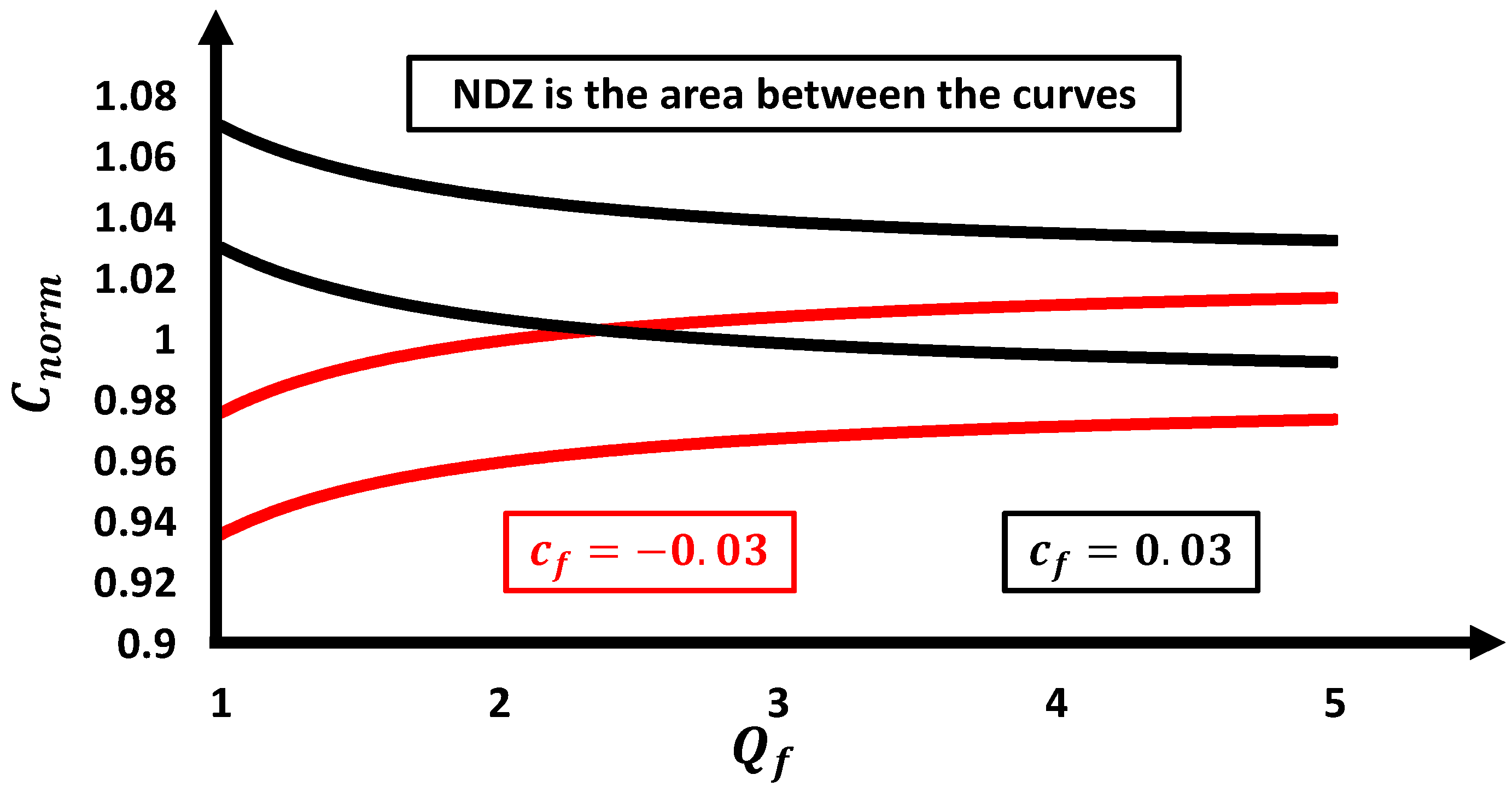
Figure 3.
SFS NDZ for different values of .

Figure 4.
behavior during the AFDPCF operation.
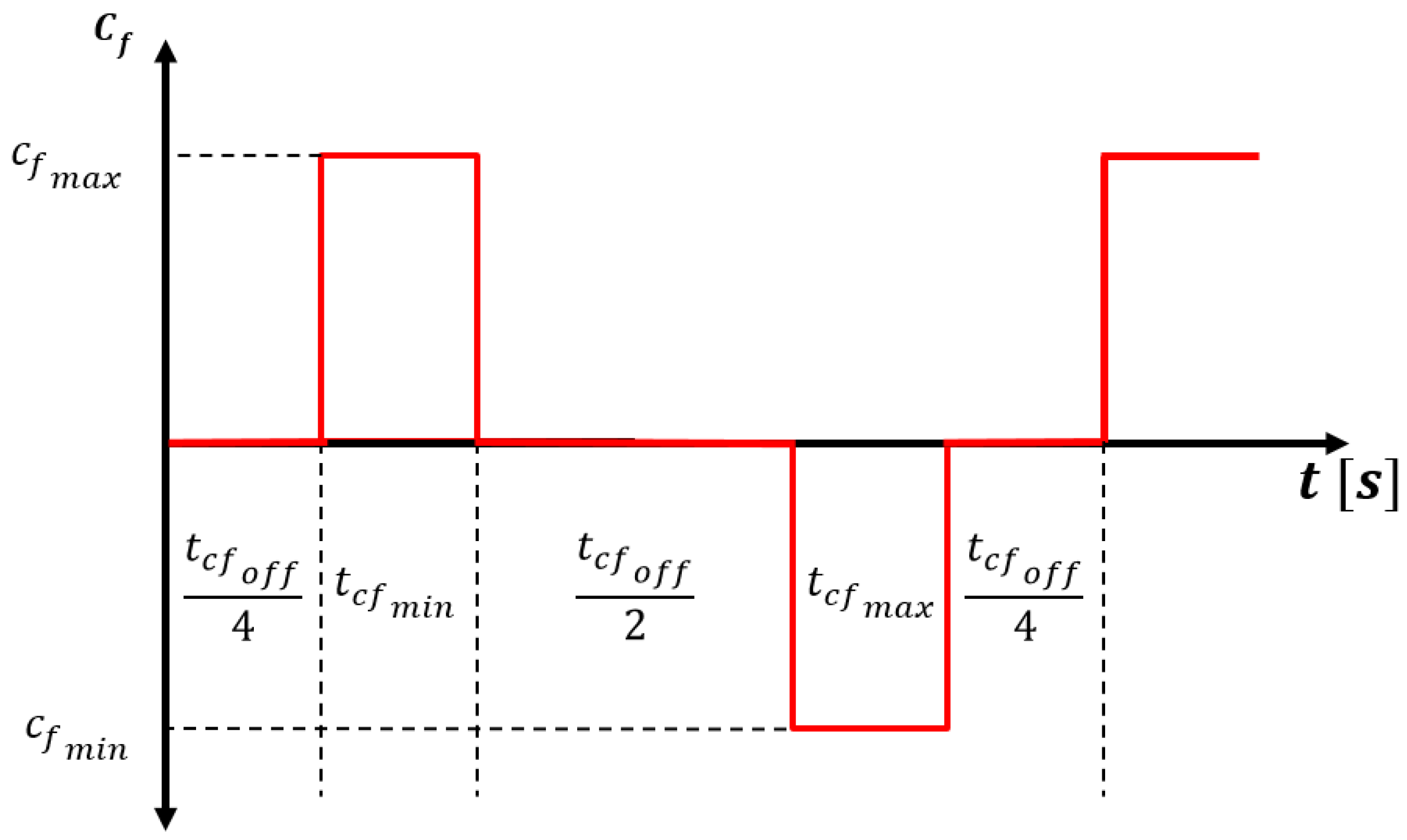
Figure 5.
AFDPCF NDZ for and .
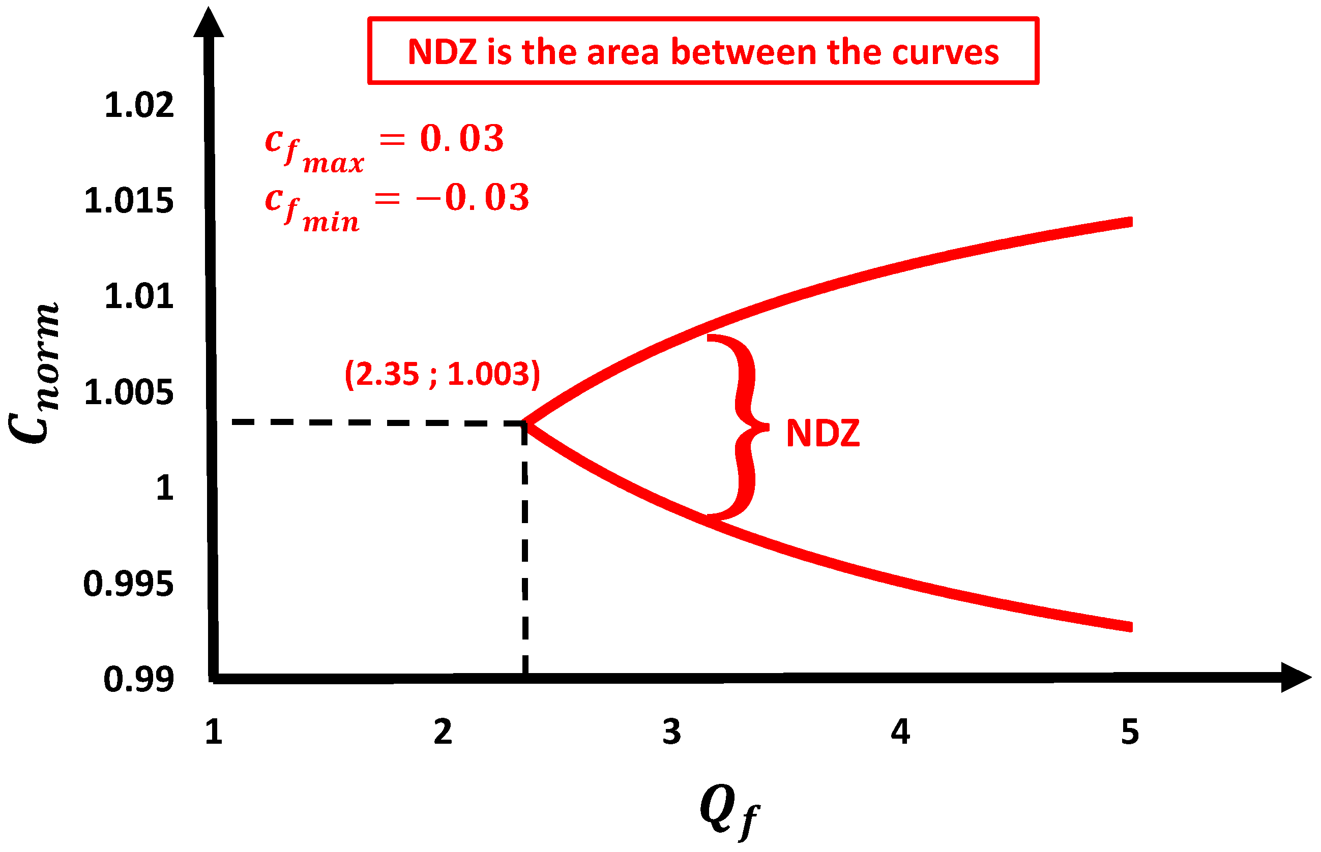
Figure 6.
AFDPCF NDZ as a project criterion: (a) AFDPCF mapping for different values of ; (b) mathematical relation versus .
Figure 6.
AFDPCF NDZ as a project criterion: (a) AFDPCF mapping for different values of ; (b) mathematical relation versus .
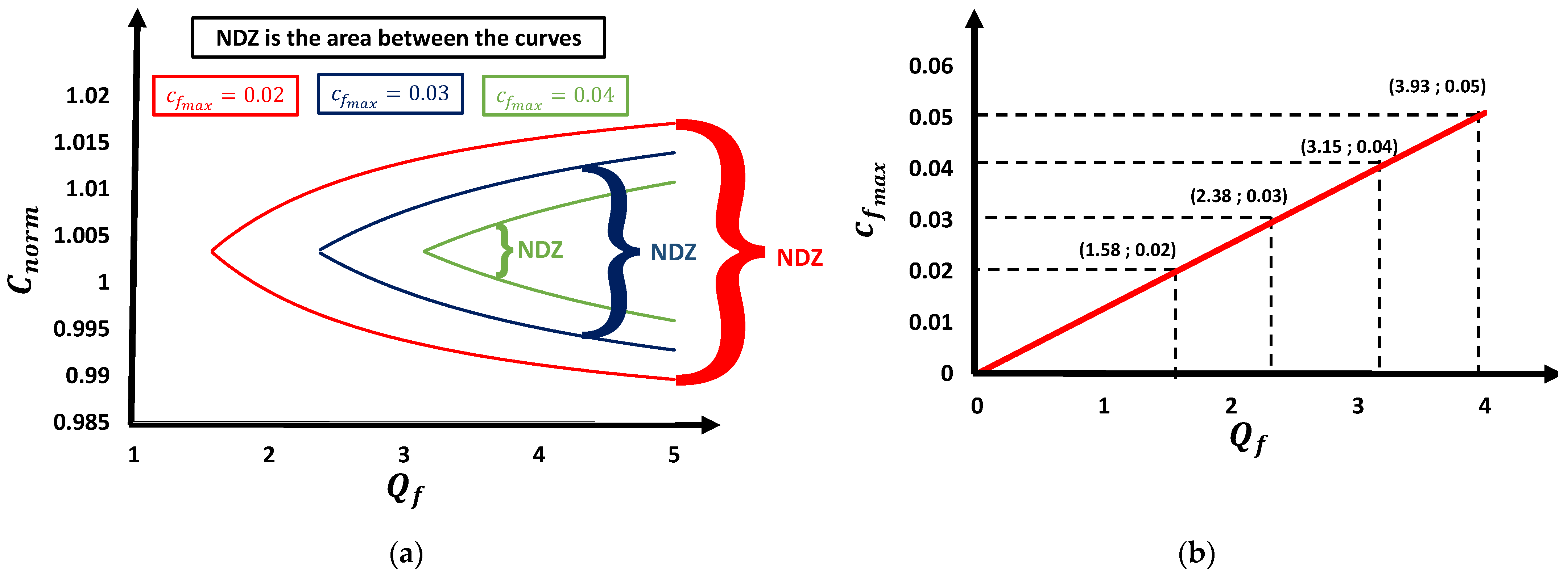
Figure 7.
Current waveform reference of the AFD proposed by [24].
Figure 7.
Current waveform reference of the AFD proposed by [24].

Figure 8.
NDZ of the AFD proposed by [24].
Figure 8.
NDZ of the AFD proposed by [24].

Figure 9.
APJPF NDZ: (a) APJPF NDZ mapping for different values of and ; (b) APJPF NDZ mapping for different values of and .
Figure 9.
APJPF NDZ: (a) APJPF NDZ mapping for different values of and ; (b) APJPF NDZ mapping for different values of and .
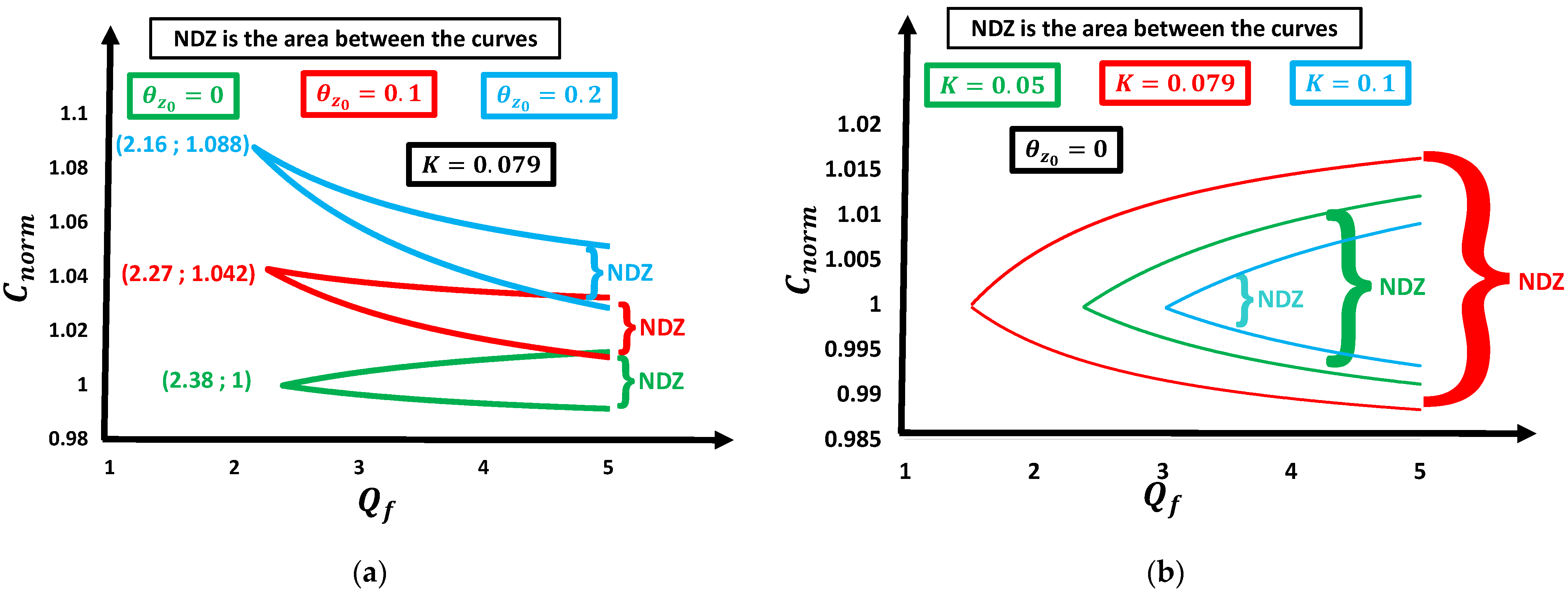
Figure 10.
Analysis of the parametrization criterion proposed by [25]: (a) Comparison of the real with the estimated value of ; (b) error of the approximation (21) in function of .
Figure 10.
Analysis of the parametrization criterion proposed by [25]: (a) Comparison of the real with the estimated value of ; (b) error of the approximation (21) in function of .
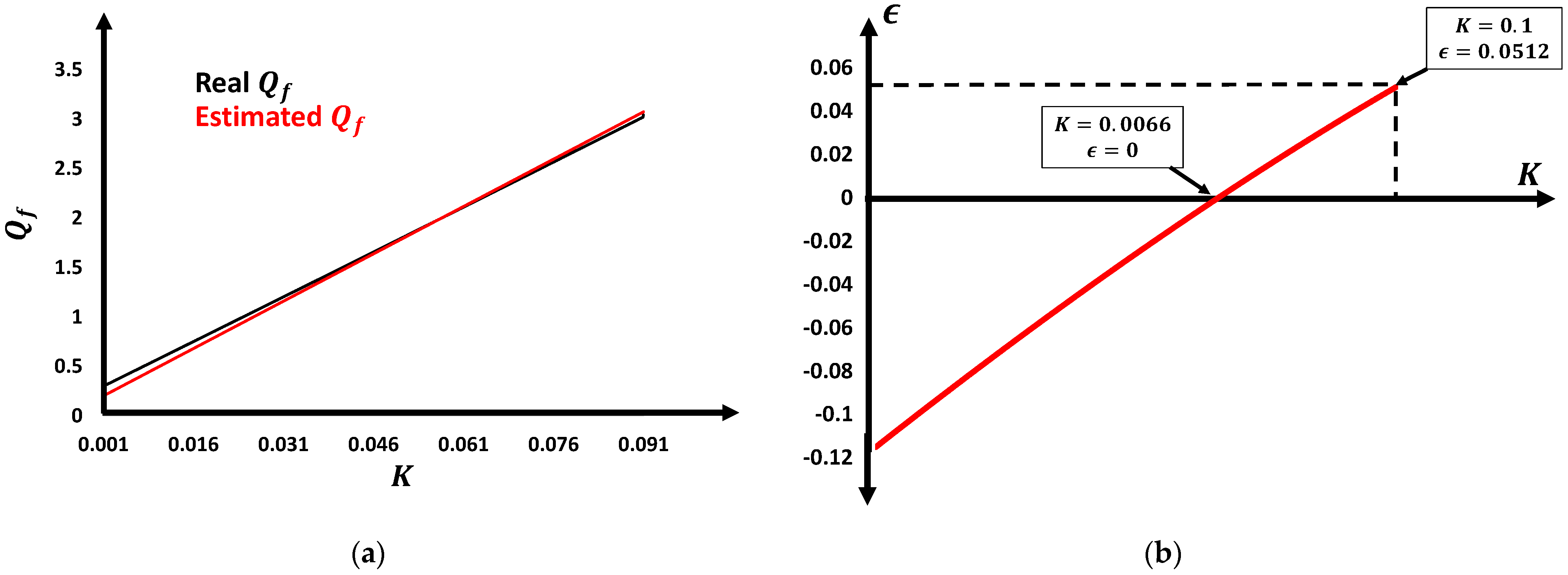
Figure 11.
Block diagram of the power and control structures.
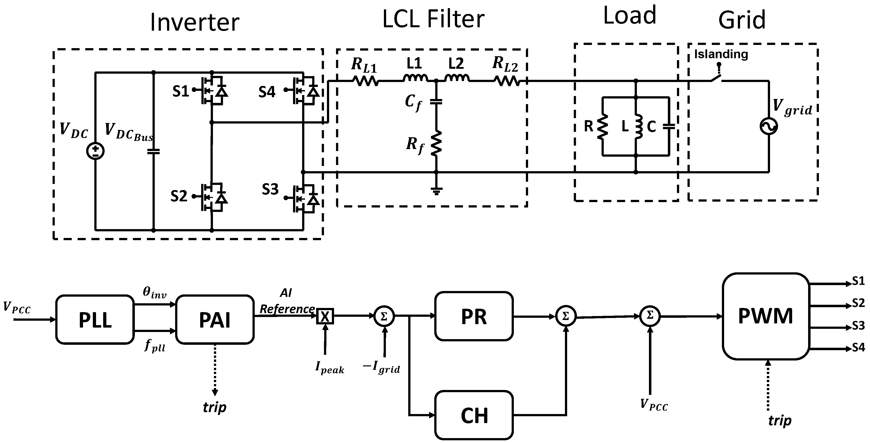
Figure 12.
Experimental implementation: (a) Inverter prototype; (b) RLC experimental load.
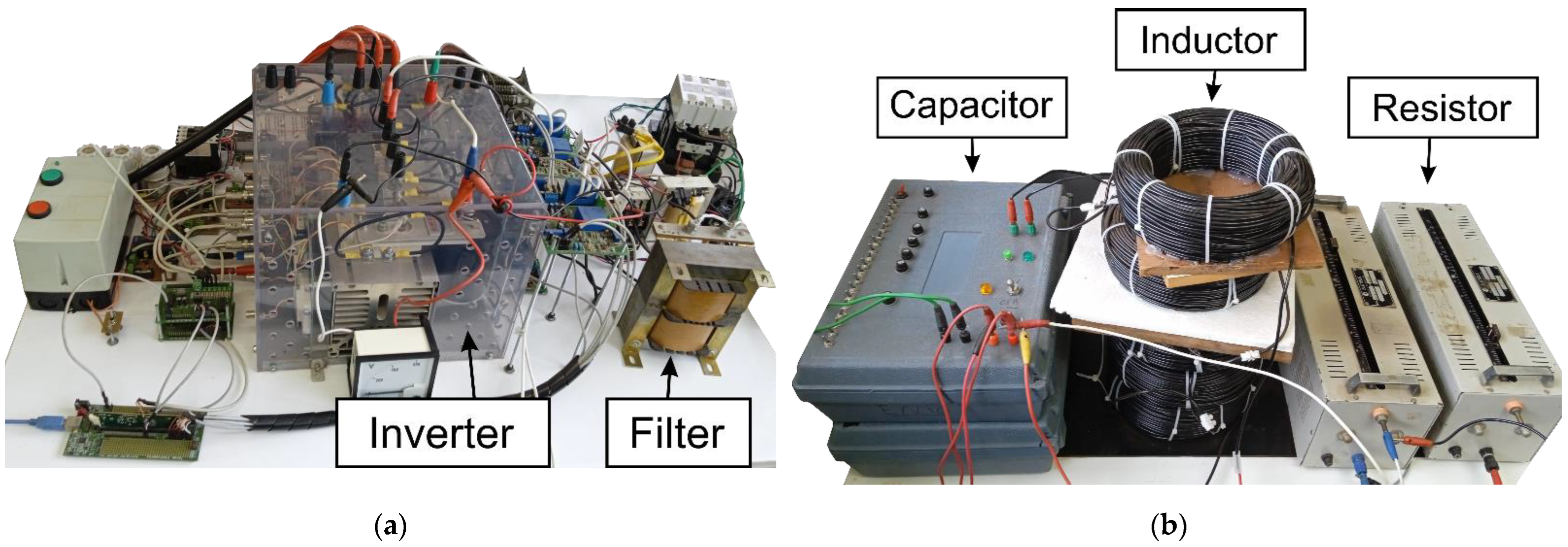
Figure 13.
Demonstration of the NDZ of the methods separated by the groups: (a) NDZ for the method of Group I; (b) NDZ for the methods of the Group II; (c) comparison of the NDZ of all of the implemented solutions [24].
Figure 13.
Demonstration of the NDZ of the methods separated by the groups: (a) NDZ for the method of Group I; (b) NDZ for the methods of the Group II; (c) comparison of the NDZ of all of the implemented solutions [24].
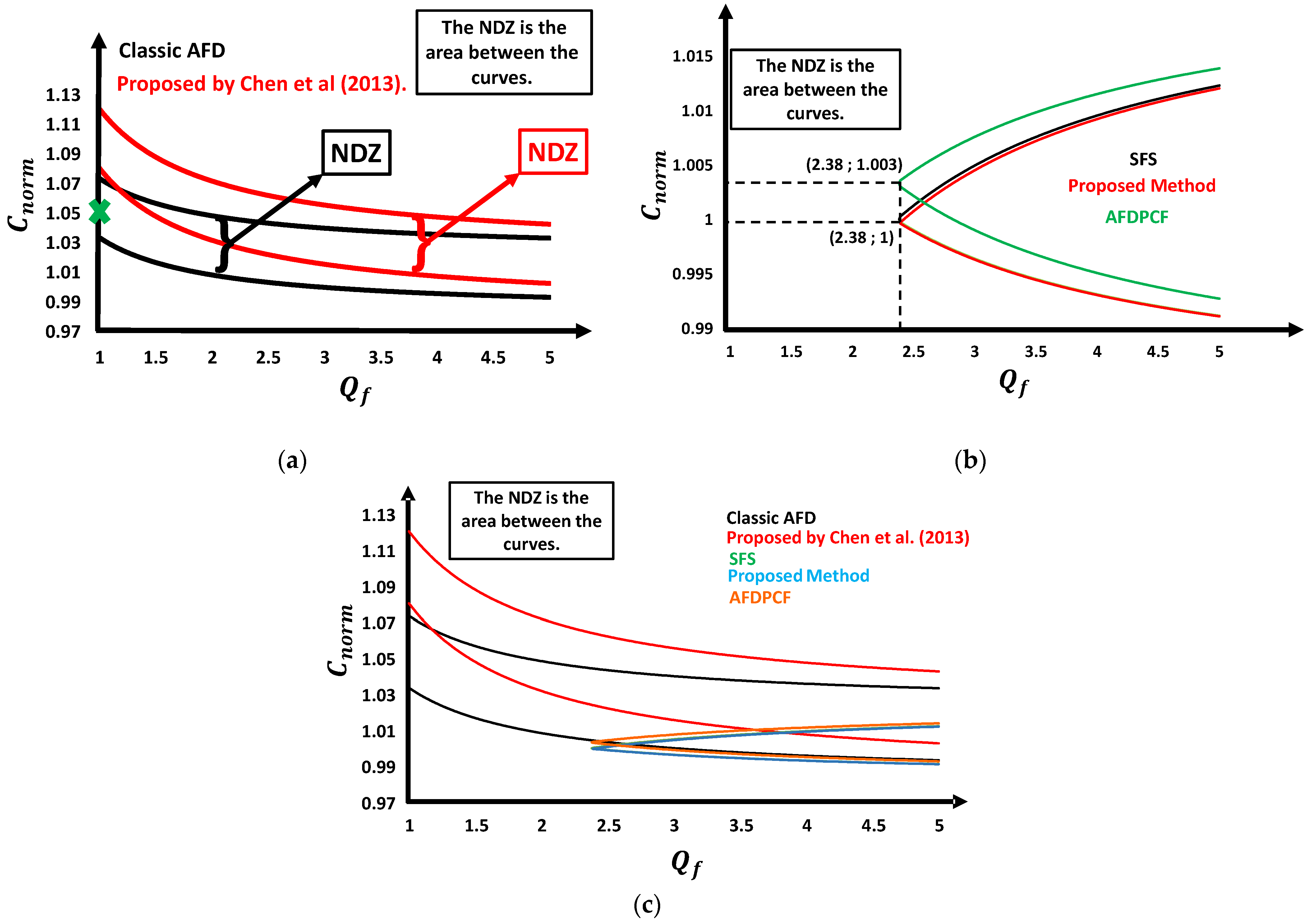
Figure 14.
Frequency, PLL Output, and Voltage Phase (a) after a positive 5 Hz frequency step; (b) after a negative 5 Hz frequency step.
Figure 14.
Frequency, PLL Output, and Voltage Phase (a) after a positive 5 Hz frequency step; (b) after a negative 5 Hz frequency step.
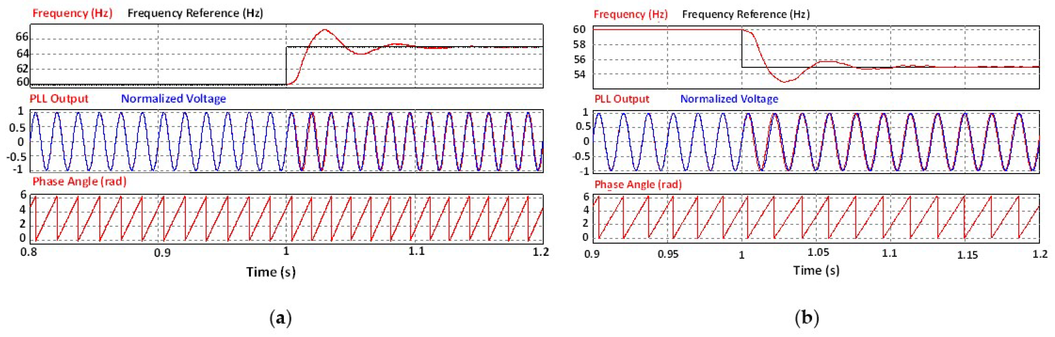
Figure 15.
Inverter output current and the current reference for: (a) a non-active AIP implemented condition; (b) a Classic AFD implemented condition; (c) an AFD proposed in Chen et al. (2013) [24] implemented condition.
Figure 15.
Inverter output current and the current reference for: (a) a non-active AIP implemented condition; (b) a Classic AFD implemented condition; (c) an AFD proposed in Chen et al. (2013) [24] implemented condition.
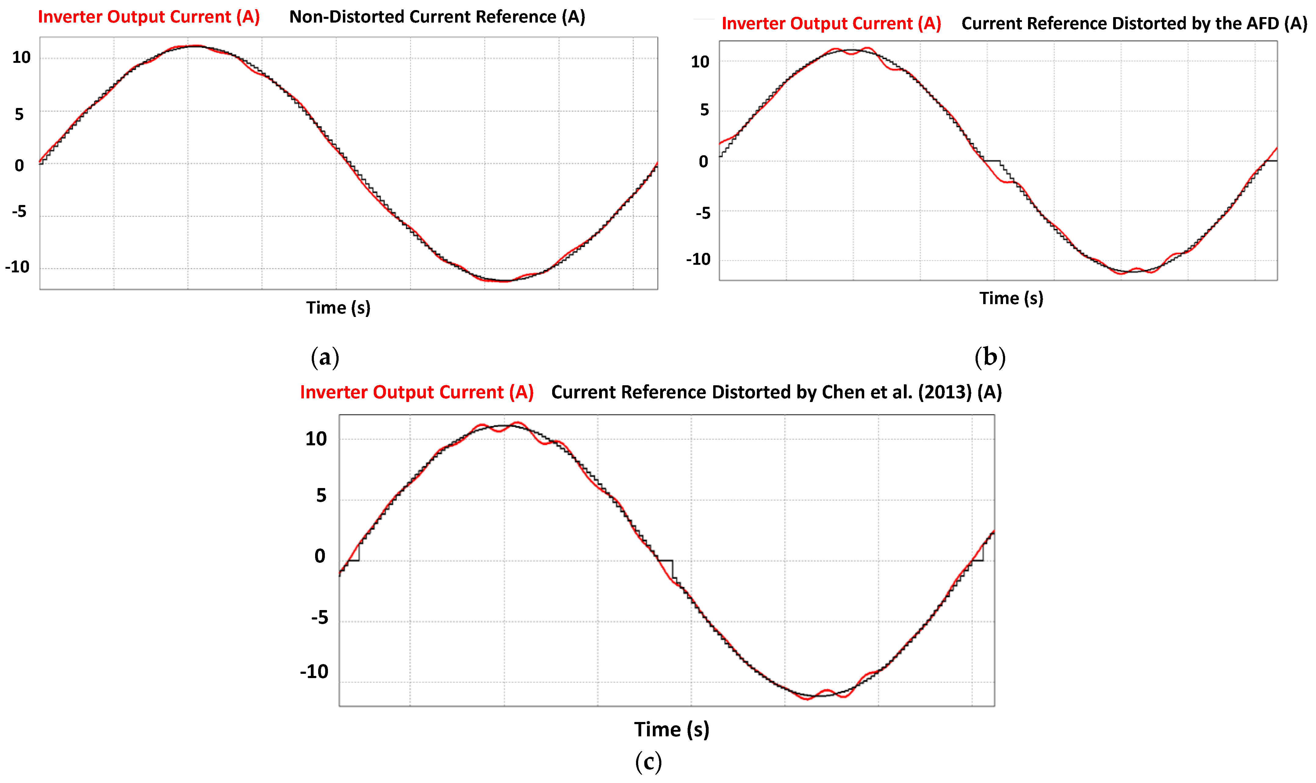
Figure 16.
Current, frequency, “Islanding”, and “Trip computational results for (a) under AFD implementation; (b) under AFD by Chen et al. (2013) [24] implementation.
Figure 16.
Current, frequency, “Islanding”, and “Trip computational results for (a) under AFD implementation; (b) under AFD by Chen et al. (2013) [24] implementation.
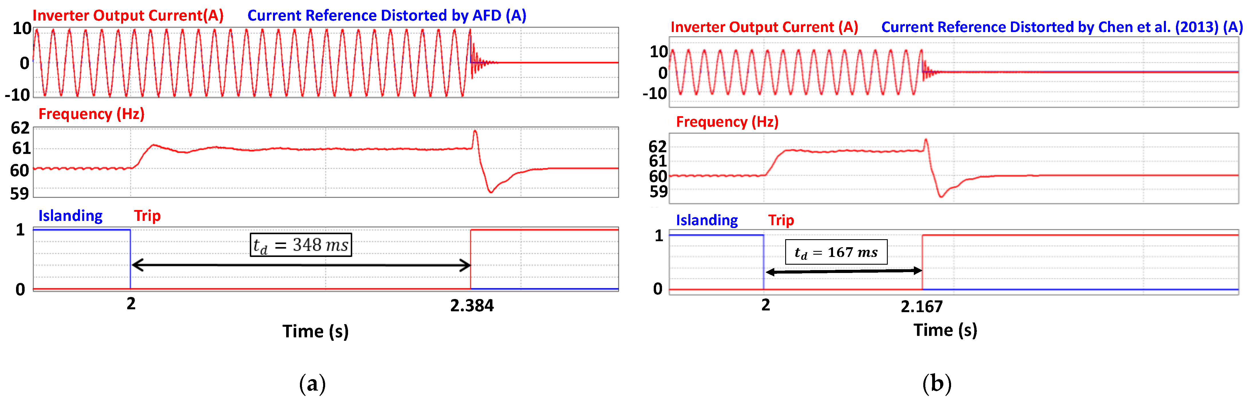
Figure 17.
Current, frequency, “Islanding”, and “Trip computational results for (a) under SFS implementation; (b) under the APJPF implementation; (c) under the AFDPCF implementation.
Figure 17.
Current, frequency, “Islanding”, and “Trip computational results for (a) under SFS implementation; (b) under the APJPF implementation; (c) under the AFDPCF implementation.
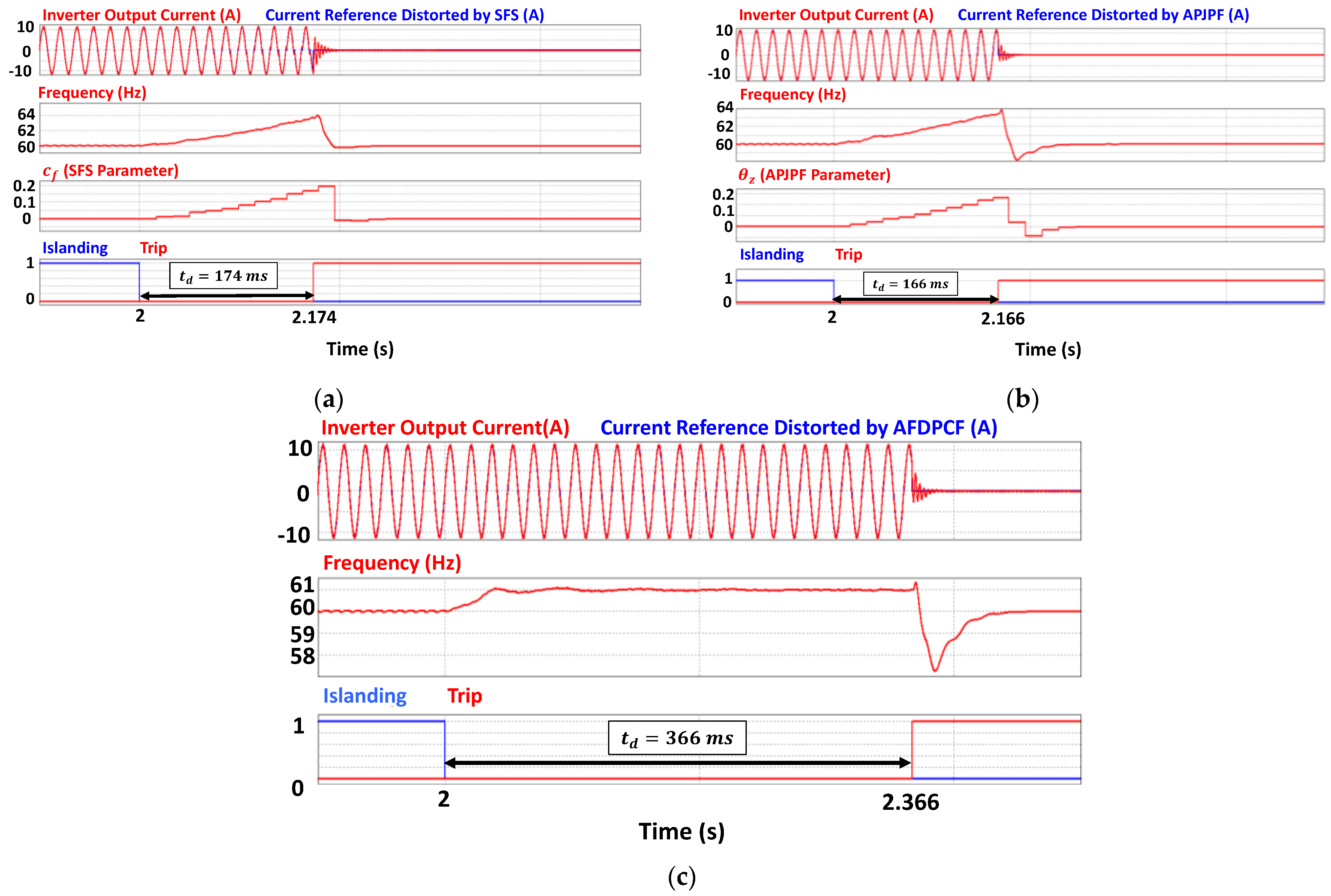
Figure 18.
Grid Current, PCC voltage, and Inverter current without the implementation of any active AIP strategy.
Figure 18.
Grid Current, PCC voltage, and Inverter current without the implementation of any active AIP strategy.

Figure 19.
Inverter current (a) under AFD implementation; (b) under AFD by [24] implementation.
Figure 19.
Inverter current (a) under AFD implementation; (b) under AFD by [24] implementation.
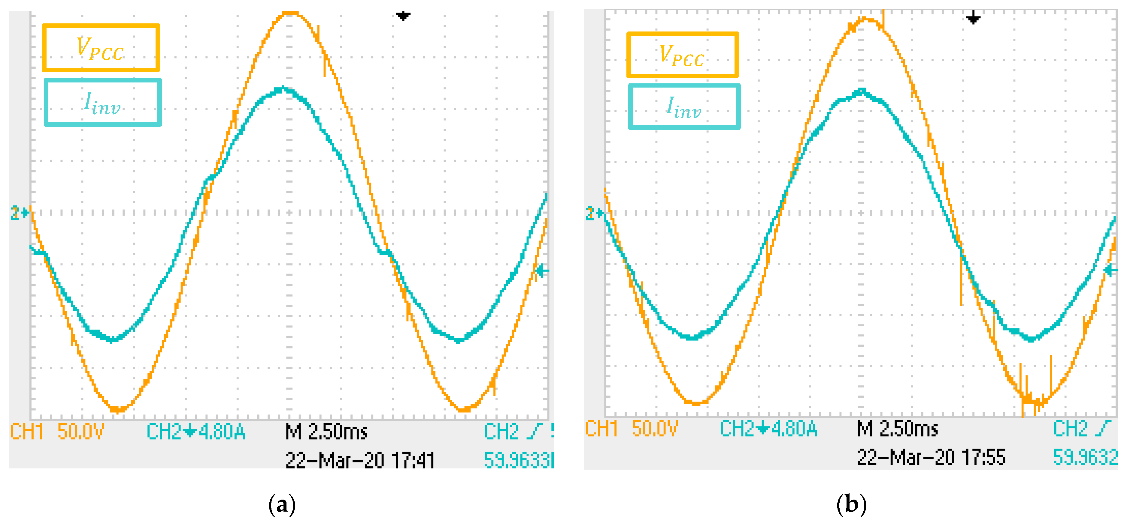
Figure 20.
PCC voltage, Inverter current, Islanding. and Trip signal (a) under AFD implementation; (b) under AFD by Chen et al. (2013) [24] implementation.
Figure 20.
PCC voltage, Inverter current, Islanding. and Trip signal (a) under AFD implementation; (b) under AFD by Chen et al. (2013) [24] implementation.

Figure 21.
Frequency behavior after the Classic AFD implementation for the .
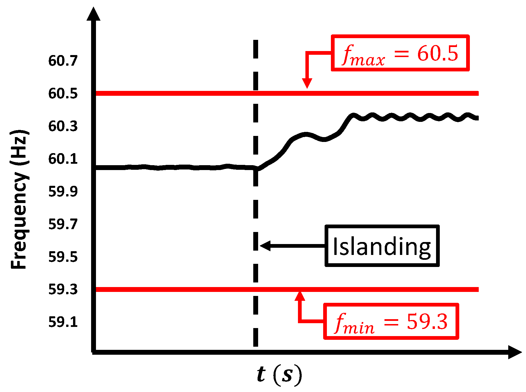
Figure 22.
PCC voltage, Inverter current, Islanding, and Trip signal (a) under SFS implementation; (b) under the APJPF implementation; (c) under AFDPCF implementation.
Figure 22.
PCC voltage, Inverter current, Islanding, and Trip signal (a) under SFS implementation; (b) under the APJPF implementation; (c) under AFDPCF implementation.
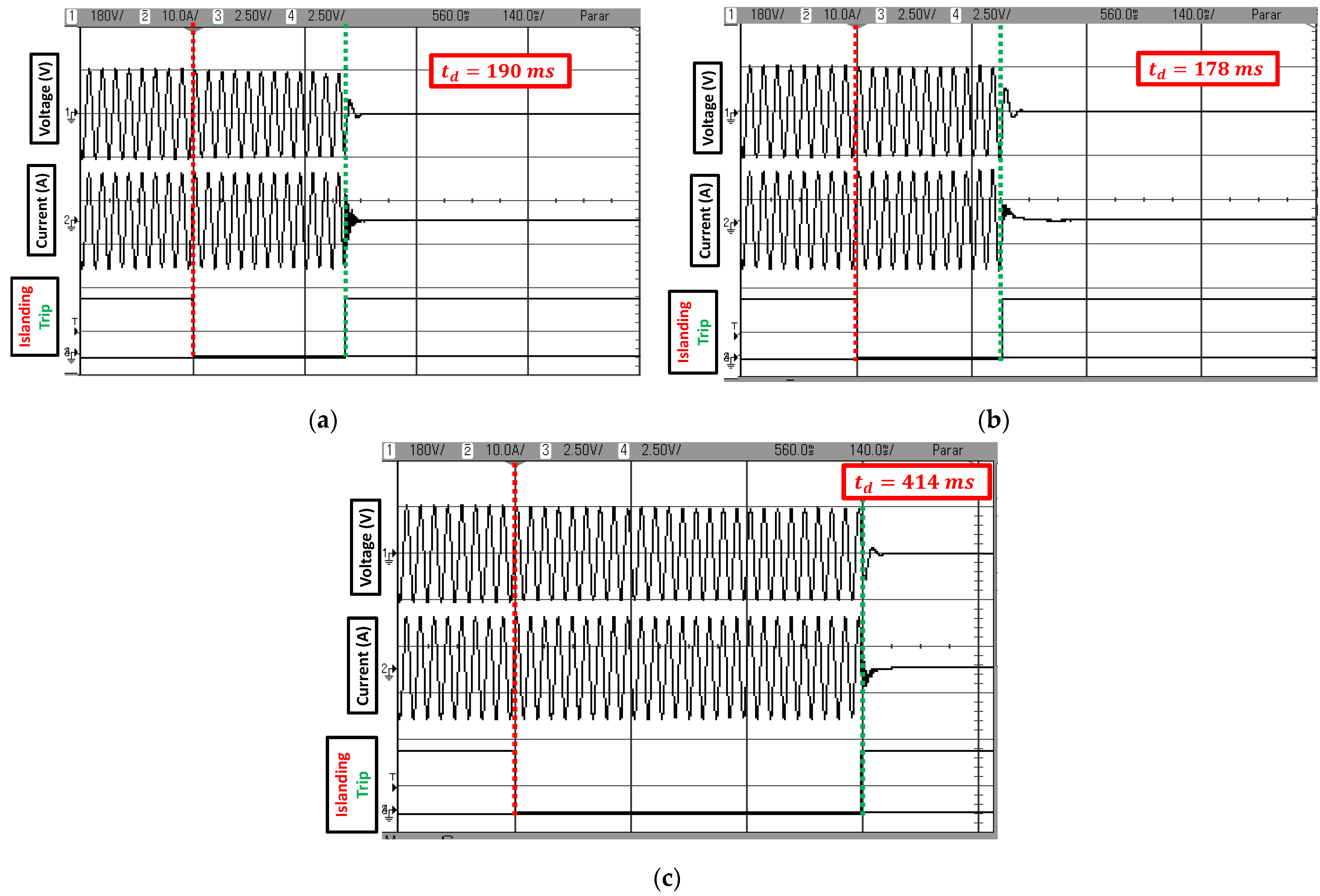
Figure 23.
Frequency behavior after the AFDPCF for .


Table 1.
Parameters of the experimental set-up implemented for anti-islanding test.
| Grid | |
|---|---|
| Rated Voltage | 127 Vrms |
| Nominal Frequency | 60 Hz |
| THDv | <2.5% |
| Inverter | |
| Output Voltage | 127 V |
| Output Current | 7.89 A |
| Rated Power | 1000 W |
| First Filter Inductor | 1.5 mH |
| First Inductor Resistance | |
| Second Filter Inductor | 10.5 mH |
| Second Inductor Resistance | 0.05 Ω |
| Dampping Resistor | 2 Ω |
| Filter Capacitor | |
| Switching Frequency | 10 kHz |
| Load | |
| Type | Parallel RLC |
| Total Resistance | 16.129 Ω |
| Total Inductance | 42.48 mH |
| Total Capacitance | |
| Resonance Frequency | 60.05 Hz |
| Quality Factor | 1.01 |
| Electrical Variable | IEEE 929–2000 | IEEE 1547–2003 | ABNT 16149 | |||
|---|---|---|---|---|---|---|
| Voltage | Range (%) | Time (s) | Range (%) | Time (s) | Range (%) | Time (s) |
| V < 50 | 0.1 | V < 50 | 0.16 | - | - | |
| 50 ≤ V ≤ 88 | 2 | 50 ≤ V < 88 | 2 | V < 80 | 0.4 | |
| 88 ≤ V ≤ 110 | 88 ≤ V ≤ 110 | 80 ≤ V ≤ 110 | ||||
| 110 ≤ V ≤ 137 | 2 | 110 ≤ V < 120 | 1 | 110 < V | 0.2 | |
| 137 ≤ V | 0.1 | V ≥ 120 | 0.16 | - | - | |
| Frequency | Range (Hz) | Time (s) | Range (Hz) | Time (s) | Range (Hz) | Time (s) |
| f < 59.5 | 0.1 | f < 59.3 | 0.16 | f < 58.5 | 0.2 | |
| f > 60.5 | 0.1 | f > 60.5 | 0.16 | f > 61.5 | 0.2 | |
| TDHv | Total | 5 % | Total | 5 % | Total | <5% |
Table 3.
Synthesis of the main performance indicators of the analyzed AIP methods.
| Groups | Methods | THDi | Detection Time | Detection Time | Detection Time |
|---|---|---|---|---|---|
| I | Classic AFD | 4.72% | 166 ms | 348 ms | Not Detected |
| Proposed by [24] | 3.18% | 113 ms | 167 ms | 351 ms | |
| II | SFS | 2.75% | 96 ms | 174 ms | 236 ms |
| AFDPCF1 | 3.15% | 171 ms | 366 ms | 566 ms | |
| AFDPCF2 | 166 ms | 315 ms | 913 ms | ||
| AFDPCF3 | 176 ms | 551 ms | 580 ms | ||
| APJPF | 2.73% | 88 ms | 166 ms | 182ms |
Table 4.
Synthesis of the main experimental results of the analyzed AIP methods.
| Groups | Methods | THDi | Detection Time | Detection Time | Detection Time |
|---|---|---|---|---|---|
| I | Classic AFD | 4.57% | 134 ms | 222 ms | Not Detected |
| Proposed in [24] | 2.56% | 100 ms | 140 ms | 264 ms | |
| II | SFS | 2.41% | 110 ms | 190 ms | 194 ms |
| AFDPCF | 3.58% | ||||
| APJPF | 2.34% | 96 ms | 178 ms | 166 ms |
Publisher’s Note: MDPI stays neutral with regard to jurisdictional claims in published maps and institutional affiliations. |
© 2022 by the authors. Licensee MDPI, Basel, Switzerland. This article is an open access article distributed under the terms and conditions of the Creative Commons Attribution (CC BY) license (https://creativecommons.org/licenses/by/4.0/).
Share and Cite
MDPI and ACS Style
Resende, Ê.C.; de Moura Carvalho, H.T.; Freitas, L.C.G. Implementation and Critical Analysis of the Active Phase Jump with Positive Feedback Anti-Islanding Algorithm. Energies 2022, 15, 4609. https://doi.org/10.3390/en15134609
AMA Style
Resende ÊC, de Moura Carvalho HT, Freitas LCG. Implementation and Critical Analysis of the Active Phase Jump with Positive Feedback Anti-Islanding Algorithm. Energies. 2022; 15(13):4609. https://doi.org/10.3390/en15134609
Chicago/Turabian StyleResende, Ênio Costa, Henrique Tannús de Moura Carvalho, and Luiz Carlos Gomes Freitas. 2022. "Implementation and Critical Analysis of the Active Phase Jump with Positive Feedback Anti-Islanding Algorithm" Energies 15, no. 13: 4609. https://doi.org/10.3390/en15134609
Note that from the first issue of 2016, this journal uses article numbers instead of page numbers. See further details here.