Bayesian Inference of Cavitation Model Coefficients and Uncertainty Quantification of a Venturi Flow Simulation

Abstract

In the present work, uncertainty quantification of a venturi tube simulation with the cavitating flow is conducted based on Bayesian inference and point-collocation nonintrusive polynomial chaos (PC-NIPC). A Zwart–Gerber–Belamri (ZGB) cavitation model and RNG k-ε turbulence model are adopted to simulate the cavitating flow in the venturi tube using ANSYS Fluent, and the simulation results, with void fractions and velocity profiles, are validated with experimental data. A grid convergence index (GCI) based on the SLS-GCI method is investigated for the cavitation area, and the uncertainty error (U_G) is estimated as 1.12 × 10⁻⁵. First, for uncertainty quantification of the venturi flow simulation, the ZGB cavitation model coefficients are calibrated with an experimental void fraction as observation data, and posterior distributions of the four model coefficients are obtained using MCMC. Second, based on the calibrated model coefficients, the forward problem with two random inputs, an inlet velocity, and wall roughness, is conducted using PC-NIPC for the surrogate model. The quantities of interest are set to the cavitation area and the profile of the velocity and void fraction. It is confirmed that the wall roughness with a Sobol index of 0.72 has a more significant effect on the uncertainty of the cavitating flow simulation than the inlet velocity of 0.52.

1. Introduction

Recently, uncertainty quantification (UQ) in computational fluid dynamics (CFD) has become an important issue in the improvement of computational performance and the reduction in computational cost in many engineering problems, such as hypersonic flow simulation for aero vehicles [1], heat and fluid flow simulations in nuclear reactors [2], and blood flow simulation in the vessels [3], etc.

Uncertainty quantification methodology can be divided into two types, depending on the presence or absence of a feedback process of statistical random inputs—the forward problem and the inverse problem [4]. The forward problem sets up the probability distribution of random inputs, calculates the amount of propagation of the inputs to the output, and calculates the quantities of interest (QoI) based on the selected UQ method. However, in the reverse problem, Bayesian inference is applied to estimate the statistics of random inputs, called a posterior distribution, using observation data with experimental or synthetic data.

In the case of the forward problem, Shaefer et al. [5] adopted the point-collocation nonintrusive polynomial chaos (PC-NIPC) method for aerodynamic flow simulation with turbulence models. They [5] investigated the effect of sampling a number of random inputs depending on the polynomial order and the probability distribution of aerodynamic performance according to the statistics of turbulence model coefficients. The model coefficients of the Spalart–Allmaras (SA) turbulence model and k-ω family models were assumed to be uniform distributions with reasonable intervals, and the geometry of the RAE 2822 airfoil and an axisymmetric bump were considered. The coefficients that contribute most to uncertainty in the results were presented according to each model and the adopted geometry.

Cheung et al. [4] proposed the methodology and process of Bayesian uncertainty quantification for the calibration and prediction of the model coefficients and combined them with a CFD simulation. They [4] investigated the effect of stochastic model classes with no uncertainty, independent Gaussian uncertainty, and correlated Gaussian uncertainty. The coefficients of the SA turbulence model were calibrated from the simulation of a flat plate boundary layer and its experimental data. They used a deterministic boundary layer solver directly instead of the surrogate model for the adaptive multilevel algorithm based on Markov chains. Their results emphasized the importance of model inadequacy and observation error in the uncertainty model, and the model class with correlated Gaussian uncertainty offered the best probabilistic results.

OCED Nuclear Energy Agency (NEA) published a review report on the UQ methodologies and the applicability of proposed UQ in CFD for nuclear safety and the regulation of equipment and components [6]. They divided the category of the possible application of single-phase CFD for Nuclear Reactor Safety (NRS) into domains and proposed a degree of maturity to each UQ method and proper choice depending on the subdomain. In Chapter 10 of the report [6], one case of uncertainty quantification for mixing flow CFD results was introduced. This forward problem adopted the nonintrusive generalized polynomial chaos expansion (GPCE) method and estimated the uncertainty of the predicted velocity, concentration, and turbulent quantities through comparison with experimental data in the Paul Scherer Institute GEMIX facility.

In the present work, the venturi tube, which is one of the important components in the field of in-service testing during reactor operation, is considered for Bayesian uncertainty quantification combining the CFD method.

The venturi tube includes cavitating flow where the vapor bubble is formed due to the phase change by a local pressure drop. In addition, the surface roughness may affect the venturi tube’s inherent function and operability of the safety-related system. However, the accurate prediction of the cavitating flow is still a challenging issue because of the model’s inadequacy in CFD and the measurement difficulties in experiments. This implies that the uncertainty of cavitating flow simulation inside a venturi tube installed at the in-service testing-related systems should be investigated with respect to the adopted cavitation model and operating conditions.

Barre et al. [7] conducted both the experiments and the numerical simulations on the cavitating flow with attached sheet cavitation in a venturi geometry. They proposed a new double optical probe measurement methodology and vapor detection algorithm to measure the void fraction and velocity profiles in the venturi tube. For the computational simulation, a barotropic approach and Yang and Shih k-ε turbulence model [8] were adopted. They showed that the simulation results are in good agreement with experimental data in a stable zone of cavitation but that there were some discrepancies in the flow velocity and void fraction profiles in the rear part of the cavitation sheet. Additionally, the sensitivity analysis of AMIN, the parameter which links the fluid density to the local pressure in the barotropic model, is conducted for better prediction of cavitating flow features [7].

Rodio and Congedo [9] applied a nonintrusive stochastic chaos method to the CFD solver to analyze the uncertainty affecting the prediction of cavitation flow in a venturi tube. The Schnerr and Sauer cavitation model [10] and k-ε turbulence model were employed. For uncertainty quantification, one model coefficient (η) and two flow conditions (inlet pressure and velocity) were considered as random variables. They found that the inlet boundary conditions are dominant contributors to the model uncertainty. In addition, a simple algorithm to obtain the optimized parameter of epistemic uncertainty was proposed.

Goel et al. [11] performed the model validation in a transport-based cryogenic cavitation model for a simple 2D hydrofoil and studied the cavitation model parameter and uncertainties with respect to temperature using surrogate-based global sensitivity analysis. They found that the model parameter associated with the evaporation was more dominant than the parameter of material uncertainty. The optimized model parameters of the transport-based cavitation model were presented in the cryogenic cavitation flow.

Ge et al. [12,13,14] investigated the thermal effect on hydraulic cavitation dynamics through experiments. They confirmed that the thermal effects showed a significant role and inhibited the growth of the sheet cavity as the temperature increased. Moreover, it was found that the re-entrant jet triggered the detachment of the attached cavity and unsteadiness.

In the current work, a CFD simulation for the venturi tube flow is combined with the Bayesian inference methodology to quantify the uncertainty of simulation results. First, the cavitation model coefficients are calibrated based on Bayesian inference with the experimental data from observations. Next, using the calibrated model coefficients from the previous section, the uncertainties of the simulation results are quantified using the PC-NIPC method for the forward problem. In this case, two operating conditions of the inlet velocity and the wall roughness at the venturi tube boundary are considered uncertain parameters, and the QoI are the cavitation area and the profiles of void fraction and velocity. In this regard, one of the present co-author [15,16] successfully predicted the location of flow leakage caused by the cavitation erosion and found that the averaged vapor volume fraction tended to increase as the surface roughness decreased in the multistage orifice.

This paper is organized as follows. Section 2 presents the governing equation for the simulation of the cavitation flow in the venturi tube and the overall procedure of Bayesian inference. The PC-NIPC model for the construction of the surrogate model is explained briefly. Then, the procedure to calculate the likelihood function, including model inadequacy and observation error, is presented. In Section 3, the venturi geometry and operating conditions are described, and the deterministic solution is validated through comparison with experimental data. To quantify the uncertainty of the grid resolution, the grid convergence index (GCI) is analyzed with respect to coarse, medium, and fine meshes. Section 4 presents the results of the Bayesian inference of ZGB model coefficients. In Section 5, the two operating conditions of inlet velocity and wall roughness are considered, and the uncertainty of the cavitation area is quantified for the forward problem.

2. Governing Equation and Numerical Methods

2.1. Cavitation and Turbulence Model

2D Reynolds-averaged Navier-Stokes equations are considered using the commercial CFD code ANSYS FLUENT v.19.1 [17]. To predict the cavitation phenomenon, a mixture multiphase model and Zwart–Gerber–Belamri (ZGB) cavitation model [18] are adopted. The turbulence model and wall modeling in the present work are selected based on the previous research of Barre et al. [7] and Rodio and Congedo [9]. The renormalization group (RNG) k-ε model is adopted for the turbulence model. The near-wall region is modeled by a standard wall function. The SIMPLE algorithm [19] is used for the pressure-velocity coupling, and a second-order upwind scheme is used for spatial discretization. For a better convergence rate, the pseudo-transient algorithm is adopted.

The governing equations of the ZGB model are as follows:

$$\frac{\partial }{\partial t}\left(f_v\rho \right)+\nabla ·\left(f_v\rho \overrightarrow{V_v}\right)=\nabla ·\left(\Gamma \nabla f_v\right)+R_e-R_c$$

(1)

$$R_e=F_{vap}\frac{3{\alpha }_{nuc}\left(1-{\alpha }_v\right){\rho }_v}{{\mathfrak{R}}_B}\sqrt{\frac{2\left(P_v-P\right)}{3{\rho }_l}} \left(if P\le P_v\right)$$

(2)

$$R_c=F_{cond}\frac{3{\alpha }_v{\rho }_v}{{\mathfrak{R}}_B}\sqrt{\frac{2\left(P-P_v\right)}{3{\rho }_l}} \left(if P\ge P_v\right)$$

(3)

where $f_v$ is the vapor mass fraction and $\Gamma$ is the diffusion coefficient. $R_e$ and $R_c$ represent the production and destruction terms in cavitation, respectively, with 4 model coefficients as shown in

Table 1. ZGB cavitation model coefficient [18].

${\mathfrak{R}}_{\mathit{B}}$	${\mathit{\alpha }}_{\mathit{n}\mathit{u}\mathit{c}}$	${\mathit{F}}_{\mathit{v}\mathit{a}\mathit{p}}$	${\mathit{F}}_{\mathit{c}\mathit{o}\mathit{n}\mathit{d}}$
10−6	5 × 10−4	50	1 × 10−2

. ${\mathfrak{R}}_B$ and ${\alpha }_{nuc}$ are the bubble radius and nucleation site volume fractions, respectively. $F_{vap}$ and $F_{cond}$ are evaporation and condensation coefficients which are multiplied in the production and destruction terms.

2.2. Grid Convergence Index (GCI)

A grid is generated to discretize the calculation domain in CFD. The number and quality of the grid elements will affect the accuracy and the errors in the calculation results. Therefore, an appropriate level of the grid should be considered, and GCI is used as a method to quantify the uncertainty according to the grid qualities. The GCI is an indicator of how the solution will converge with a further grid refinement by computing the percentage error between the numerical solution and the asymptotic value. Roache [20] proposed a GCI method based on Richardson’s extrapolation, but this method can be used only in the case of monotonically increasing or decreasing solutions with grid refinement. To overcome this disadvantage, Tanaka and Miyake [21] proposed the least square-based GCI (SLS-GCI) that can be applied in general CFD situations. Their equations describing grid scales are presented below.

$$r_{21}=\frac{h_2}{h_1}, r_{32}=\frac{h_3}{h_2} (h_1<h_2<h_3)$$

(4)

$${ϵ}_{21}=f_2-f_1, {ϵ}_{32}=f_3-f_2$$

(5)

where $h_k$ is the representative grid size for the three different grids (coarse, medium, and fine), $r$ is the grids ratio, $f_k$ is the prediction result of each grid, and $ϵ$ is the result difference. The order of convergence $\left(p\right)$, extrapolated value $\left(f_c\right)$, and coefficients $\left(\alpha \right)$ can be calculated as the solution of Equation (7) as follows:

$${\tilde{f}}_k=f_c+\alpha {\left(h_k\right)}^p$$

(6)

$$S={{\displaystyle \sum }}_{k=1}^3{\left\{f_k-\left[f_c-\alpha {\left(h_k\right)}^p\right]\right\}}^2$$

(7)

The GCI and error of estimation can be calculated according to the order of convergence.

$$u_G=\frac{Fs\left|{\tilde{f}}_2-{\tilde{f}}_1\right|}{r_{21}^p-1}=Fs\left|{\tilde{f}}_c-{\tilde{f}}_1\right|$$

(8)

$$u_e=\sqrt{\frac{1}{3}{{\displaystyle \sum }}_{k=1}^3{\left[f_k-\left\{f_c+\alpha h_k^p\right\}\right]}^{}}$$

(9)

2.3. Bayesian Inference

Bayesian inference is a method to address the inverse problem, where the goal is to back-propagate information about an observation to obtain insight into the uncertainty input parameter. Bayesian inference can calibrate the uncertainty input parameters from the observed data using Bayes’ theorem with prior knowledge [22].

$$p\left(\theta |d\right)=\frac{p\left(d|\theta \right)p\left(\theta \right)}{p\left(d\right)}$$

(10)

where $\theta$ are the uncertainty input parameters to be inferred and $d$ is the observation data. $p\left(\theta \right)$ is the prior distribution of the parameters that reflects the level of information existing on the parameters $\theta$ before any measurement is carried out. $p\left(d|\theta \right)$ is the likelihood (or likelihood function) that represents an estimate of a parameter, and it indicates which parameters are most likely. $p\left(d\right)$ is a normalizing factor, known as the evidence or marginal likelihood. $p\left(\theta |d\right)$ is the posterior distribution of uncertainty for the input parameters.

In the present Bayesian inference, the coefficients of the ZGB cavitation model are considered as uncertainty inputs and are calibrated using experimental observation data by Barre et al. [7]. The overall procedure and framework for Bayesian inference are adopted based on those proposed by Cheung et al. [4].

2.4. Point-Collocation Nonintrusive Polynomial Chaos (PC-NIPC)

Bayesian inference includes the process in which the statistical distribution of random inputs is calculated iteratively with a likelihood function and observation data using the specified sampling method. To apply this process in CFD fields, many simulations of the deterministic solver are required to determine the acceptance of the sampling data. When the computational time and cost of each deterministic simulation are considered, the alternative can become the surrogate model or reduced-order statistics analysis. In the present work, PC-NIPC is adopted for the construction of the surrogate model based on the simulation results with sampled inputs [23].

NIPC expansions are functional approximations of a computational model through its spectral representation on a suitably built basis of polynomial functions. The method is to define the joint probability density function (PDF) $f_X$ from a random vector with independent components $X\in {ℝ}^M$. The next step is to consider a finite variance computational model as a map $Y=\mathcal{M}\left(X\right)$, $Y\in ℝ$ such that:

$$\mathbb{E}\left[Y^3\right]={{\displaystyle \int }}_{{\mathcal{D}}_X}^{}{\mathcal{M}}^2\left(X\right)f_X\left(x\right)dx<\infty$$

(11)

Then, the polynomial chaos expansion of $\mathcal{M}\left(X\right)$ is defined as follows:

$$\mathcal{M}\left(X\right)\approx {\mathcal{M}}^{PC}\left(X\right)={\displaystyle \sum }_{\alpha \in A}{y}_{\alpha }{\psi }_{\alpha }\left(X\right) (A\subset {\mathbb{N}}^{\mathbb{M}})$$

(12)

where $y_{\alpha }\in ℝ$ are the corresponding coefficients, and $A\subset {\mathbb{N}}^{\mathbb{M}}$ is the set of selected multi-indices of multivariate polynomials. In Equation (12), ${\psi }_{\alpha }\left(X\right)$ are the multivariate polynomials that are assembled as the tensor product of their univariate counterparts, as shown in

Table 2. List of classic univariate polynomial families [5].

Type of Variable	Distribution	Orthogonal Polynomials	$\mathbf{Hilbertian} \mathbf{Basis} {\mathit{\psi }}_{\mathit{k}}\left(\mathit{x}\right)$
Uniform $\mathit{U}\left(-1,1\right)$	$\frac{\mathbf{1}\left(\mathit{x}\right)}{\mathbf{2}}$	$\mathrm{Legendre} {\mathit{P}}_{\mathit{k}}\left(\mathit{x}\right)$	${\mathit{P}}_{\mathit{k}}\left(\mathit{x}\right)$$/\sqrt{\frac{\mathbf{1}}{\mathbf{2}\mathit{k}+\mathbf{1}}}$
Gaussian $\mathit{G}\left(\mathbf{0},\mathbf{1}\right)$	$\frac{\mathbf{1}}{\sqrt{\mathbf{2}\mathit{\pi }}}{\mathit{e}}^{-{\mathit{x}}^{\mathbf{2}}/\mathbf{2}}$	$\mathrm{Hermite} {\mathit{H}}_{{\mathit{e}}_{\mathit{k}}}\left(\mathit{x}\right)$	${\mathit{H}}_{{\mathit{e}}_{\mathit{k}}}\left(\mathit{x}\right)$$/\sqrt{\mathit{k}!}$
Gamma $\Gamma \left(\mathit{a},\mathit{\lambda }=\mathbf{1}\right)$	${\mathit{x}}^{\mathit{a}}{\mathit{e}}^{-\mathit{x}}$	$\mathrm{Laguerre} {\mathit{L}}_{\mathit{k}}^{\mathit{a}}\left(\mathit{x}\right)$	${\mathit{L}}_{\mathit{k}}^{\mathit{a}}\left(\mathit{x}\right)$$/\sqrt{\frac{\Gamma \left(\mathit{k}+\mathit{a}+\mathbf{1}\right)}{\mathit{k}!}}$
Beta $\mathit{B}\left(\mathit{a},\mathit{b}\right)$	$\mathbf{1}\left(\mathit{x}\right)\frac{{\left(\mathbf{1}-\mathit{x}\right)}^{\mathit{a}}{\left(\mathbf{1}+\mathit{x}\right)}^{\mathit{b}}}{\mathit{B}\left(\mathit{a}\right)\mathit{B}\left(\mathit{b}\right)}$	$\mathrm{Jacobi} {\mathit{J}}_{\mathit{k}}^{\mathit{a},\mathit{b}}\left(\mathit{x}\right)$	${\mathit{J}}_{\mathit{k}}^{\mathit{a},\mathit{b}}\left(\mathit{x}\right)$$/{\mathfrak{J}}_{\mathit{a},\mathit{b},\mathit{k}}$

.

In the present study, the PC-NIPC method, which was proposed by Hosder et al. [23], is adopted. For adoption of the PC-NIPC, the minimum sampling number of random input variables is calculated by Equation (13), with the polynomial order (p), the number of random input variables (n), and the oversampling rate (n_p). Hosder et al. [23] recommended that the oversampling rate should be more than 2 for a better approximation with the given polynomial order.

$$P+1=n_p\frac{\left(n+p\right)!}{n!p!}$$

(13)

2.5. Source of Uncertainty

2.5.1. Model Inadequacy

Cheung et al. [4] mentioned that not only is a description of the uncertainty related to the model coefficients but also that a description of the uncertainty regarding the model itself is important. Because the turbulent model coefficients are derived from the assumption of relatively simple flows, such as isotropic turbulence and boundary layer flows, there is a limit to accurately reflecting complex turbulence phenomena in real engineering problems. This model inadequacy becomes a source of uncertainty that propagates through the computational model and leads to errors in the predictions of the model.

In the current work, the model inadequacy of the cavitation model is considered. Assuming $\tilde{d}$ as the true process with no error, the computational model $\mathcal{M}\left(X\right)$ and the model inadequacy $\eta$ can be related as follows:

$$\tilde{d}=\mathcal{M}\left(X\right)+\eta$$

(14)

Cheung et al. [4] suggested a three-model classification of model inadequacy (no uncertainty, independent Gaussian uncertainty, and correlated Gaussian uncertainty). The correlated Gaussian uncertainty showed the highest posterior plausibility among these model classes [24].

$$\eta ~Gaussian \left(0,K_{\eta }\right), K_{\eta }={\sigma }_{\eta }^{2}exp\left[-\frac{1}{2}{\left(\frac{x-x^{\prime }}{l}\right)}^2\right]$$

(15)

$${\sigma }_{\eta }~Uniform\left(0, 0.1\right)$$

(16)

2.5.2. Observation Error

Observation error is one of the unavoidable uncertainties in experimental works. When the parameter uncertainty is calibrated by experimental data corresponding to the observation, modeling the observation error is an important process in Bayesian inference. However, since information on the error bars of the experimental data [7], which are adopted as observations in this simulation, and the data behind these error bars were not provided, the model was assumed to be an independent Gaussian model by Cheung et al. [4]. The true process $\tilde{d}$, observation error $e$, and observation data $d$ can be related as follows:

$$d=\tilde{d}+e$$

(17)

$$e~Gaussian\left(0,K_e\right), K_e={\sigma }_e^{2}I$$

(18)

$${\sigma }_e~Uniform\left(0, 0.02\right)$$

(19)

where $K_e$ is a diagonal matrix with each diagonal component equal to the variance. Observation errors are independent Gaussian random variables with zero mean and standard deviation.

2.6. Likelihood Function

All stochastic models are combined into the likelihood function. From Equations (14) and (17), observation data can be expressed by a conditional Gaussian distribution as follows:

$$d|\sigma ,X ~ Gaussian\left(\mathcal{M}\left(X\right),K\right))$$

(20)

where $\sigma$ is the uncertainty parameter including ${\sigma }_e$ and ${\sigma }_{\eta }$, and $K$ is the covariance matrix that is the sum of $K_{\eta }+K_e$. Finally, if all the inferred uncertainty parameters ($\sigma ,X$) are applied as inputs to find $\theta$, the likelihood function and posterior distribution can be expressed as follows:

$$P\left(d|\theta \right)=\frac{1}{Z}\frac{1}{\sqrt{{\left(2\pi \right)}^{N}det\left(K\right)}}exp\left(-\frac{1}{2}{\left(d-\mathcal{M}\left(X\right)\right)}^T{K}^{-1}\left(d-\mathcal{M}\left(X\right)\right)\right)$$

(21)

$$Z={{\displaystyle \int }}^{ }P(d|\theta )P\left(\theta \right)d\theta$$

(22)

$$P\left(\theta |d\right)=\frac{1}{Z}\frac{1}{\sqrt{{\left(2\pi \right)}^{N}det\left(K\right)}}exp\left(-\frac{1}{2}{\left(d-\mathcal{M}\left(X\right)\right)}^T{K}^{-1}\left(d-\mathcal{M}\left(X\right)\right)\right)P\left(\theta \right)$$

(23)

2.7. Markov Chain Monte Carlo (MCMC)

In practice, posterior distributions do not have a closed-form solution. One widely used option to solve inverse problems relies upon the MCMC model [25]. The basic idea of MCMC simulations is to construct a Markov chain that equals the posterior distribution over the prior support ${\mathcal{D}}_X$. Markov chains can be uniquely defined by their transition probability $\mathcal{K}\left(x^{\left(t+1\right)}|x^{\left(t\right)}\right)$ from the step $x^{\left(t\right)}$ of the chain at iteration t to the step $x^{\left(t+1\right)}$ at the subsequent iteration $t+1$. Then, the posterior is equal to the Markov chain if the specified transition probability fulfills the detailed balance condition:

$$\pi \left(x^{\left(t\right)}|y\right) \mathcal{K}\left(x^{\left(t+1\right)}|x^{\left(t\right)}\right)=\pi \left(x^{\left(t+1\right)}|y\right) \mathcal{K}\left(x^{\left(t\right)}|x^{\left(t+1\right)}\right)$$

(24)

One of the algorithms to fulfill this equation is the Metropolis–Hastings (MH) algorithm [26] which is based on proposing and subsequently accepting or rejecting candidate points. At iteration t from the current sample $x^{\left(t\right)}$, one then draws a candidate sample $x^{(\star )}$ from a proposal distribution $p\left(x^{(\star )}|x^{\left(t\right)}\right)$. Subsequently, the candidate is accepted with a probability as follows:

$$\alpha \left(x^{(\star )},x^{\left(t\right)}\right)=\min \left\{1,\frac{\pi \left(x^{(\star )}|\mathcal{Y}\right)p\left(x^{\left(t\right)}|x^{(\star )}\right)}{\pi \left(x^{\left(t\right)}|\mathcal{Y}\right)p\left(x^{(\star )}|x^{\left(t\right)}\right)}\right\}$$

(25)

However, most MCMC algorithms perform poorly when the target distribution shows strong correlations between the parameters. A considerable amount of tuning is necessary to improve the performance of these algorithms. The affine invariant ensemble (AIES) algorithm [27] alleviates this problem by assuming solutions that are invariant with affine transformations of the target distribution. The affine invariance property is achieved by generating proposals according to a so-called stretch move. This refers to proposing a new candidate by:

$$x_i^{(\ast )}=x_i^{\left(t\right)}+Z\left(x_j^{\left(t\right)}-x_i^{\left(t\right)}\right), where Z~p\left(z\right)=\{\begin{array}{c}\frac{1}{\sqrt{z}\left(2\sqrt{a}-\frac{2}{\sqrt{a}}\right)} if z\left[\frac{1}{a},a\right]\\ 0 otherwise\end{array}$$

(26)

This requires sampling from the distribution p(z) defined by the tuning parameter $a>1$. The candidate $x_i^{(\ast )}$ is then accepted as the new location of the i-th walker, with a probability given as follows:

$$\alpha \left(x_i^{(\ast )}, x_i^{\left(t\right)}, z\right)=\min \left\{1,z^{M-1}\frac{\pi \left(x_i^{(\ast )}|\mathcal{Y}\right)}{\pi \left(x_i^{\left(t\right)}|\mathcal{Y}\right)}\right\}$$

(27)

3. Deterministic Simulation

3.1. Geometry and Operating Condition

The two-dimensional geometry is adopted from the experiment of Barre et al. [7]. The height at the venturi throat is 43.7 mm, and the convergence and divergence angles are 4.3° and 4.0°, respectively, as shown in Figure 1. The detailed geometric information is presented in

Table 3. Geometric parameters.

$$\begin{gathered} S_{\mathrm{inlet}} \\ \left(\mathbf{mm}\right) \end{gathered}$$	$$\begin{gathered} S_{\mathrm{throat}} \\ \left(\mathbf{mm}\right) \end{gathered}$$	$$\begin{gathered} S_{\mathrm{outlet}} \\ \left(\mathbf{mm}\right) \end{gathered}$$	$$\begin{gathered} L_x \\ \left(\mathbf{mm}\right) \end{gathered}$$	Convergence Angle (°)	Divergence Angle (°)
50.0	43.7	60.2	1512	4.3	4.0

. The conditions of temperature, fluid density, and viscosity of water and vapor are set as shown in

Table 4. Fluid properties.

Water Property		Vapor Property
${\rho }_l$ $(kg/m^3)$	${\mathsf{\mu }}_{\mathbf{l}}$ $(kg/\left(m·s\right))$	${\mathsf{\rho }}_{\mathbf{l}}$ $(kg/m^3)$	${\mathsf{\mu }}_{\mathbf{l}}$ $(kg/m·s)$
998.2	$1.002 \times {10}^{-3}$	998.2	$1.002 \times {10}^{-3}$

. The velocity at the inlet is set to 10.8 m/s and the pressure at the outlet to 38,450 Pa, shown in

Table 5. Operating conditions.

Velocity Inlet	Pressure Outlet	Saturated Pressure
10.8 m/s	38,450 Pa	2339 Pa

, the same as the experimental condition of Barre et al. [7]. A no-slip boundary condition is applied to the solid wall. The saturated pressure for the prediction of cavitation is given as 2339 Pa.

From the grid test, which will be explained in Section 3.3, the medium mesh (29,536 nodes) is selected for the present simulation. When it is considered that the mesh size of Barre et al. [7] is 9,861 nodes, the adopted mesh in the present simulation is adequate to simulate the steady sheet cavitation.

3.2. Validation of the Deterministic Simulation

Deterministic simulation is validated by the experimental data and numerical simulation result of Barre et al. [7]. Figure 2 shows the comparison of the void fraction and longitudinal velocity (u-velocity) at the stations of X = 5.1 mm, 38.4 mm, and 73.9 mm from the venturi throat. Barre et al. [7] presented two velocity profiles from the experiment; one is the mean velocity (Vmean), and the other is the most probable velocity (Vmp). The most probable velocity (Vmp) is calculated from the probability density function of the measured velocity, which is one of the techniques to predict the velocity in a bubble flow. They showed that mean velocity (Vmean) and the most probable velocity (Vmp) were not similar because of the unsteady behavior of a vapor bubble with high intermittency. The two velocity profiles are presented for comparison with the simulation results.

The void fraction of a vapor bubble at the wall decreases with an increase in the distance from the venturi throat and is measured as about zero at the station of X = 73.9 mm. The prediction of the void fraction shows good agreement with experimental data at the stations of X = 5.1 mm and 73.9 mm. The thickness and distribution of a vapor bubble show consistent behavior with reference [7] at both positions. However, the simulated void fraction at X = 38.4 mm is similar to that of the numerical simulation by Barre et al. [7]. This overprediction of the void fraction below y~4 mm in two simulation results seems to be due to the limit of multiphase mixture modeling, and this trend is also shown in the simulation results of Rodio and Congedo [9]. In contrast, the simulation result by Barre et al. [7] showed a still large vapor region at the station of X = 73.9 mm; the present simulation is able to predict the thickness and the distribution of a vapor bubble in a manner that agrees with the experimental data.

The velocity profiles predicted by the present simulation show a large discrepancy at the station of X = 5.1 mm and 38.4 mm, which is quite similar to the results by Rodio and Congedo [9]. In the simulation by Barre et al. [7], a new extended wall function [28] was adopted to model the turbulent boundary layer, and this model enhanced the prediction of the boundary layer profile relative to the present result. When it is considered that there is also a big difference between two experimental data points, Vmean and Vmp, the prediction of the velocity inside the vapor is still a challenging problem. In the present simulation, one encouraging result is the accurate prediction of the recirculation zone in the wake at the third station (X = 73.9 mm).

The contour of the void fraction and the longitudinal velocity are presented in Figure 3. As shown in the void fraction contour, as the distance from the venturi throat increases, the thickness of the cavity sheet increases. The length of the sheet, which is determined with the threshold of 0.3 of void fraction, is predicted as 75.0 mm, with a 6.3% difference from the measured value, 80 mm [7]. The velocity contour shows the recirculation zone in the back region of the vapor sheet, which is consistent with the velocity profile at X = 73.9 mm in Figure 2.

3.3. Grid Convergence Index (GCI)

GCI based on the SLS-GCI method [21] is investigated using a coarse, medium, and fine meshes presented in

Table 6. Grid test results.

	Coarse	Medium	Fine
Number of nodes	16,027	29,536	59,492
Cavitation area(m2)	2.57 × 10−4	2.52 × 10−4	2.51 × 10−4

. The number of nodes in the medium and fine meshes increases by 1.8 and 3.7 times, respectively, compared with the coarse mesh. To evaluate the GCI, the cavitation area, which is calculated with the integration of the cell area with the void fraction below 0.3, is selected as the QoI. The GCI results are summarized in

Table 7. Grid Convergence Index results.

${\mathit{f}}_{\mathit{c}}$	${\mathit{U}}_{\mathit{e}}$	${\mathit{U}}_{\mathit{G}}$
2.53 × 10−4	4.22 × 10−6	1.12 × 10−5

. The extrapolation values ($f_c$), which mean an estimate of the cavitation area at zero grid spacing, error of estimation ($U_e$), which means the difference between numerical and estimated results, and the uncertainty from the grid ($U_G$) are presented in this table. The cavitation area is extrapolated as 2.53 × 10⁻⁴ at zero grid spacing, and the error and uncertainty between both results are 4.22 × 10⁻⁶ and 1.12 × 10⁻⁵, respectively. It is judged that the grid test results are reasonable and that the selection of a medium mesh is appropriate in the current work.

4. Bayesian Inference of ZGB Model Coefficients

In this section, the Bayesian inference of ZGB model coefficients is conducted following the procedure presented in Section 2.3. The first step for Bayesian inference is to determine the random inputs and their prior distribution. In the present work, four coefficients of the ZGB cavitation model are selected as the random inputs, as shown in

Table 8. The prior distribution interval of random parameters.

Parameter	Lower Boundary	Upper Boundary
${\mathfrak{R}}_B$~Uniform	2.0 × 10−7	1.0 × 10−6
${\alpha }_{nuc}$~Uniform	0.00025	0.0006
$F_{vap}$~Uniform	25	55
$F_{cond}$~Uniform	0.005	0.015
${\sigma }_{\eta }$~Uniform	0	0.3
${\sigma }_e$~Uniform	0	0.05

. Additionally, two more parameters of model inadequacy and observation error are considered. Because of the lack of knowledge of the model coefficients, it is assumed that these have a uniform distribution. Edeling et al. [29] mentioned that the prior interval of random inputs was selected based on three factors: the spreads of coefficients proposed by the original model, the ranges of these for which the solution was stable, and the avoidance of apparent truncation of the posterior at the edge of the prior range. Since the range of the model coefficients was not presented in the original literature, Zwart et al. [18], the range of each coefficient is initially guessed as ±50% with respect to the original mean initial value. However, since the posterior probability distribution through the calibration procedure is not constrained to the initial prior intervals, the prior range is modified with a wider one or is translated with proper values, as recommended by Edeling et al. [29]. The final ranges of the prior distribution of the four model coefficients are shown in Table 8.

The next step is to construct the surrogate model based on PC-NIPC [23] using the sampling data of the random inputs. The calculated sampling number based on PC-NIPC is 30 with a second-order polynomial, two chosen for the oversampling rate, and four random variables.

$$P\left(d|\theta \right)=\frac{1}{Z}\frac{1}{\sqrt{{\left(2\pi \right)}^N\mathit{det}\left(K\right)}}exp\left(-\frac{1}{2}{\left(d-\mathcal{M}\left(X\right)\right)}^T{K}^{-1}\left(d-\mathcal{M}\left(X\right)\right)\right)$$

(28)

$$K=K_{\eta }+K_e, K_{\eta }={\sigma }_{\eta }^{2}exp\left[-\frac{1}{2}{\left(\frac{x-x^{\prime }}{l}\right)}^2\right], K_e={\sigma }_e^{2}I$$

(29)

where $K$ is the covariance matrix of the summation $K_{\eta }$ model inadequacy and $K_e$ observation error [4]. Details regarding the prior distribution are shown in Table 8.

The void fraction profile in the experiment [7] is set to QoI with the assumed error of ±5% and then is adopted as the observation data for Bayesian inference.

To obtain the sample of the posterior distribution, the AIES [27] algorithm is employed with 500 parallel runs of 2000 steps. Each PDF of a parameter was approximated by a kernel density estimation with half of the sample burn-in. After Bayesian inference based on the mentioned procedures, the calibrated model coefficients can be obtained. The posterior distributions of the calibrated coefficients are shown in Figure 4, and the posterior mean values are presented in

Table 9. Posterior mean values of model coefficients.

ZGB Coefficients	${\mathfrak{R}}_{\mathit{B}}$	${\mathit{\alpha }}_{\mathit{n}\mathit{u}\mathit{c}}$	${\mathit{F}}_{\mathit{v}\mathit{a}\mathit{p}}$	${\mathit{F}}_{\mathit{c}\mathit{o}\mathit{n}\mathit{d}}$
Nominal value	10−6	5 × 10−4	50	0.01
Posterior Mean	7.9 × 10−7	4.5 × 10−4	52	0.013

.

As shown in Figure 4, the calibrated coefficients are constrained inside the finial prior interval, which means the prior range of the model coefficients is appropriate. The posterior means of ${\mathfrak{R}}_B$ and ${\alpha }_{nuc}$ are decreased from their nominal values, but the posterior means of $F_{vap}$ and $F_{cond}$ are increased after Bayesian inference considering the profile of void fraction as QoI. Since the peak of the void fraction at X = 73.9 mm is predicted to be 75% larger than the original ZGB model coefficients, Bayesian inference adopting the experimental data of the void fraction profile as observation data makes the calibrated model coefficients predict smaller values. The coefficient, ${\alpha }_{nuc}$, in the ZGB model is related to the production term, and the decrease in this coefficient induces smaller production in the governing Equation (1). The coefficients of $F_{vap}$ and $F_{cond}$ are multiplied in production and destruction terms, respectively. It should be noted that $F_{vap}$ is calibrated as the value 52, larger than the original value of 50, which is a small increase of 4%. In contrast, the coefficient $F_{cond}$ is increased by 30% from 0.01 to 0.013 and then induces an increase in the destruction of cavities.

The void fraction and velocity profiles with the calibrated model coefficients at the station of X = 73.9 mm are presented with the experimental data [7] and the simulation result with the original coefficients in Figure 5. The prediction of the void fraction is 75% better than that of the original prediction, and the velocity profile is still able to correctly predict the recirculation zone. At the other two stations (X = 5.1 and 38.4 mm), there is a small difference, within 2%, in the void fraction and velocity profiles between both cases. This means that the calibrated model coefficients have little effect on the flow properties of the upstream part. If the velocity profile is adopted as observation data, the model coefficients will be calibrated for a better prediction of the velocity profile. Figure 6 shows the contours of the void fraction with the calibrated model coefficients. It is confirmed that the cavitation area and the sheet length are smaller than the values predicted by the original model.

5. Uncertainty Quantification with Respect to Operating Conditions

In this section, the uncertainty with respect to the operating conditions in the venturi tube is quantified based on the calibrated ZGB model coefficients. Overall procedures of the corresponding forward problem are (1) the selection of random variables and the determinations of the distributions and their ranges, (2) the definition of QoI, (3) the sampling of random variables depending on the polynomial order and number of inputs, (4) construction of the PC-NIPC model [23], and (5) the calculation of the statistical distribution of QoI and postprocessing.

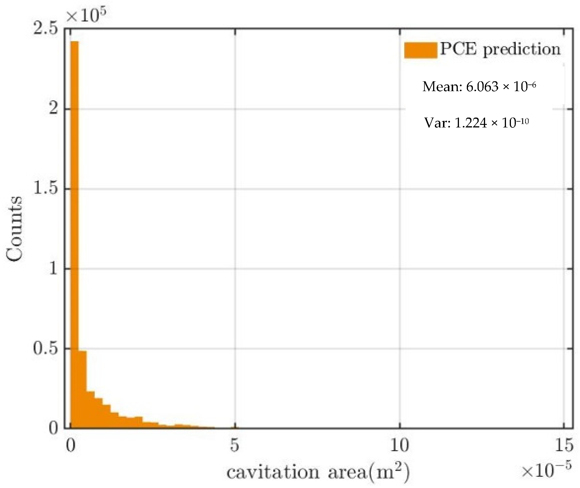
The considered uncertain input variables are the inlet velocity and the roughness of the wall, which are known as important parameters influencing the flow characteristics of a venturi tube [30,31]. The inlet velocity is modeled as a Gaussian distribution with 10% variation with respect to the given condition, 10.8 m/s. The wall roughness is assumed to be uniform from 0.0001 m to 0.001 m, as shown in Figure 7. In the present work, a wall roughness of zero, an ideally smooth wall, is not considered from the engineering point of view. The QoI is set to the cavitation area for direct comparison with the previous simulation result. The sampling number is determined from 12 to 112, considering the polynomial order from second to sixth orders and the oversampling rate from 2 to 4 for the two input variables and one QoI. The Latin hypercube sampling methodology is adopted to sample random variables, and the PC-NIPC model is constructed for the surrogate model depending on the polynomial order. The leave-one-out (Loo) error, which is an indicator of the proper polynomial order and sampling number, has a minimum of 2.13 × 10⁻² at the fourth polynomial order and an oversampling rate of 4. Figure 8 shows the histogram of the cavitation area, which is the QoI in the present section, according to the variation of operating conditions. The distribution of the cavitation area is similar to an exponential distribution which peaks at areas close to the order of 10⁻⁶ m². The mean of the cavitation area (6.063 × 10⁻⁶ m²) is reduced by 42 times compared with the deterministic solution (2.52 × 10⁻⁴ m²) for the fixed velocity and smooth wall.

Additionally, the sensitivity of input variables is analyzed using the Sobol index. The Sobol indices of the inlet velocity and wall roughness are calculated as 0.59 and 0.72, respectively. This means that the roughness has much more effect on the cavitation area, the QoI, than the inlet velocity.

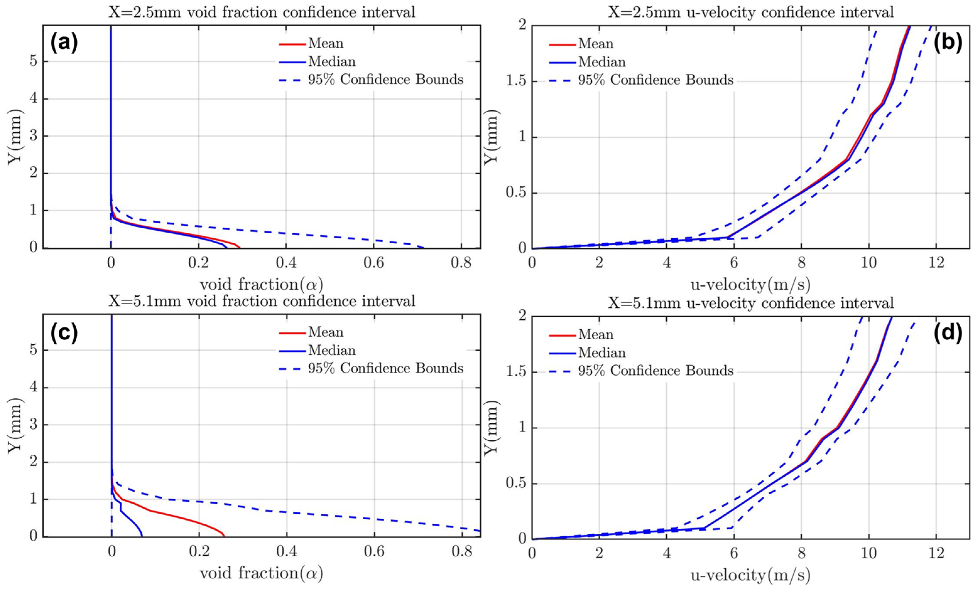
Figure 9 shows the profile of the void fraction and the longitudinal velocities at the two stations of X = 2.5 mm and 5.1 mm. The mean and median values of both are respectively presented in black and orange lines, and the dashed line corresponds to the 95% confidence bound as a result of the uncertainty quantification. In the void fraction profile, there are large 95% confidence bounds starting from 0 to 0.9. However, the velocity profiles show a 95% confidence interval within 10% of the mean value. This means that the wall roughness has a very large effect on the ZGB cavitation model, and the cavitation behavior is affected by the wall roughness. Further investigation of the uncertainty quantification between the cavitation model and wall roughness seems to be necessary. The median area of the void fraction at X = 5.1 mm is predicted to be as small as one-third of the mean value, which means that the distribution of the cavitation area resembles the exponential function.

The contours of the void fraction and longitudinal velocity are presented in Figure 10. It is confirmed that the length of the cavitation sheet is shortened before X = 38.4 mm and that a recirculation zone is shown near X = 38.4 mm.

6. Conclusions

In the present work, Bayesian inference of the cavitation model coefficients is conducted in the venturi tube flow, and the calibrated model coefficients are applied to the venturi tube flows, which have the same geometry and flow condition as those in Barre et al. [7].

To validate the deterministic solution, the profiles of the void fraction and longitudinal velocity at three stations are compared with experimental data and simulation results by Barre et al. [7]. The void fraction profiles agree well with the reference ones at the front two stations and show better prediction than the simulation result by Barre et al. [7]. The prediction of the turbulent boundary layer inside and outside cavitating zone fails, which is consistent with Rodio and Congedo’s [9] simulation results, but the recirculation zone is predicted correctly.

GCI analysis by the SLS-CGI method [21] is conducted with respect to the global parameters and cavitation area and shows 2.53 × 10⁻⁴ for the extrapolation value (f_c), 4.22 × 10⁻⁶ for the estimation error (U_e), and 1.12 × 10⁻⁵ for the uncertainty error (U_G). In addition, it is confirmed that the adopted medium mesh with a value approximately equal to the cavitation area of 2.52 × 10⁻⁴ is appropriate.

For Bayesian inference of ZGB model coefficients, four model coefficients are calibrated, and the covariance matrix, which is proposed by Cheung et al. [4], including model inadequacy and observation error, is considered. After initial guesses of the uniform prior intervals of (±50%) of each model coefficient, the range of each is modified with the criteria that the posterior range by Bayesian inference should be constrained inside the prior one. Posterior means of ${\mathfrak{R}}_B$ and ${\alpha }_{nuc}$ are decreased from their nominal values, but posterior means of $F_{vap}$ and $F_{cond}$ are increased to decrease the void fraction at the third station at X = 73.8 mm. The velocity profile at all stations shows little change after Bayesian inference. However, there are still large discrepancies in the prediction of velocity and void fraction after observation data are accounted for by Bayesian inference. This means that the perturbation of cavitation model coefficients is not sufficient to remedy the model deficiency. In future work, the other parameters, such as turbulence model inadequacy and discretization error, should be considered simultaneously as uncertain inputs for Bayesian inference [32,33].

Finally, the forward problem with respect to the operating conditions, including the inlet velocity and the wall roughness, is conducted based on the PC-NIPC model with a fourth-order polynomial and an oversampling rate of 4. Therefore, 60 cases are sampled with the Latin hypercube sampling method. When the uncertainty of the wall roughness is considered, in contrast with the previous general simulation with a smooth wall, the cavitation area is decreased 42 times, and the variation of the void fraction is very large, ranging from 0 to 0.9. The discrepancy between the mean and median value of the void fraction is observed. Through the sensitivity analysis with the Sobol index, the wall roughness (0.72) has more effect on the simulation result than the inlet velocity (0.59). This means that the wall roughness in the venturi-type components of the in-service testing should be considered carefully to obtain consistent results with the experiment and quantify the uncertainty of performance in the venturi tube.

References

- West, T.K., IV; Hosder, S. Uncertainty quantification of hypersonic reentry flows with sparse sampling and stochastic expansions. J. Spacecr. Rocket. 2015, 52, 120–133. [Google Scholar] [CrossRef]
- Zeng, K.; Hou, J.; Ivanov, K.; Jessee, M.A. Uncertainty quantification and propagation of multiphysics simulation of the pressurized water reactor core. Nucl. Technol. 2019, 205, 1618–1637. [Google Scholar] [CrossRef]
- Sankaran, S.; Kim, H.J.; Choi, G.; Taylor, C.A. Uncertainty quantification in coronary blood flow simulations: Impact of geometry, boundary conditions and blood viscosity. J. Biomech. 2016, 49, 2540–2547. [Google Scholar] [CrossRef] [PubMed]
- Cheung, S.H.; Oliver, T.A.; Prudencio, E.E.; Prudhomme, S.; Moser, R.D. Bayesian uncertainty analysis with applications to turbulence modeling. Reliab. Eng. Syst. Saf. 2011, 96, 1137–1149. [Google Scholar] [CrossRef]
- Schaefer, J.; Hosder, S.; West, T.; Rumsey, C.; Carlson, J.R.; Kleb, W. Uncertainty quantification of turbulence model closure coefficients for transonic wall-bounded flows. AIAA J. 2017, 55, 195–213. [Google Scholar] [CrossRef]
- Bestion, D.; De Crecy, A.; Moretti, F.; Camy, R.; Barthet, A.; Bellet, S.; Munoz Cobo, J.; Badillo, A.; Niceno, B.; Hedberg, P.; et al. Review of uncertainty methods for CFD application to nuclear reactor thermal hydraulics. In Proceedings of the NUTHOS 11-the 11th International Topical Meeting on Nuclear Reactor Thermal Hydraulics, Operation and Safety, Gyeongju, Korea, 9–13 October 2016. [Google Scholar]
- Barre, S.; Rolland, J.; Boitel, G.; Goncalves, E.; Patella, R.F. Experiments and modeling of cavitating flows in venturi: Attached sheet cavitation. Eur. J. Mech.-B/Fluids 2009, 28, 444–464. [Google Scholar] [CrossRef] [Green Version]
- Shih, T.H.; Liou, W.W.; Shabbir, A.; Yang, Z.; Zhu, J. A new k-ϵ eddy viscosity model for high Reynolds number turbulent flows. Comput. Fluids 1995, 24, 227–238. [Google Scholar] [CrossRef]
- Rodio, M.G.; Congedo, P.M. Robust analysis of cavitating flows in the venturi tube. Eur. J. Mech.-B/Fluids 2014, 44, 88–99. [Google Scholar] [CrossRef]
- Schnerr, G.H.; Sauer, J. Physical and numerical modeling of unsteady cavitation dynamics. In Fourth International Conference on Multiphase Flow; ICMF New Orleans: New Orleans, LO, USA, 2001. [Google Scholar]
- Goel, T.; Thakur, S.; Haftka, R.T.; Shyy, W.; Zhao, J. Surrogate model-based strategy for cryogenic cavitation model validation and sensitivity evaluation. Int. J. Numer. Methods Fluids 2008, 58, 969–1007. [Google Scholar] [CrossRef] [Green Version]
- Ge, M.; Sun, C.; Zhang, G.; Coutier-Delgosha, O.; Fan, D. Combined suppression effects on hydrodynamic cavitation performance in Venturi-type reactor for process intensification. Ultrason. Sonochem. 2022, 86, 106035. [Google Scholar] [CrossRef]
- Ge, M.; Zhang, G.; Petkovšek, M.; Long, K.; Coutier-Delgosha, O. Intensity and regimes changing of hydrodynamic cavitation considering temperature effects. J. Clean. Prod. 2022, 338, 130470. [Google Scholar] [CrossRef]
- Ge, M.; Petkovšek, M.; Zhang, G.; Jacobs, D.; Coutier-Delgosha, O. Cavitation dynamics and thermodynamic effects at elevated temperatures in a small Venturi channel. Int. J. Heat Mass Transf. 2021, 170, 120970. [Google Scholar] [CrossRef]
- Lee, G.; Bae, J. Numeircal study of the effect of the surface roughness magnitude on the multi-stage orifice internal flow pattern. Am. Nucl. Soc. Trans. 2021, 124, 748–751. [Google Scholar]
- Lee, G.; Jhung, M.; Bae, J.; Kang, S. Numerical Study on the Cavitation Flow and Its Effect on the Structural Integrity of Multi-Stage Orifice. Energies 2021, 14, 1518. [Google Scholar] [CrossRef]
- ANSYS. ANSYS Fluent Theory Guide. 2019. Available online: http://www.ansys.com/ (accessed on 26 April 2022).
- Zwart, P.J.; Gerber, A.G.; Belamri, T. A two-phase flow model for predicting cavitation dynamics. In Proceedings of the Fifth International Conference on Multiphase Flow, Yokohama, Japan, 30 May–3 June 2004. [Google Scholar]
- Patankar, S.V.; Spalding, D.B. A calculation procedure for heat, mass and momentum transfer in three-dimensional parabolic flows. In Numerical Prediction of Flow, Heat Transfer, Turbulence and Combustion; Elsevier: Amsterdam, The Netherlands, 1983; pp. 54–73. [Google Scholar]
- Roache, P.J. Quantification of uncertainty in computational fluid dynamics. Annu. Rev. Fluid Mech. 1997, 29, 123–160. [Google Scholar] [CrossRef] [Green Version]
- Tanaka, M.; Miyake, Y. Numerical simulation of thermal striping phenomena in a T-junction piping system for fundamental validation and uncertainty quantification by GCI estimation. Mech. Eng. J. 2015, 2, 15–134. [Google Scholar] [CrossRef] [Green Version]
- Kaipio, J.; Somersalo, E. Statistical and computational inverse problems. In Applied Mathematical Sciences; Springer: Berlin/Heidelberg, Germany, 2005; p. 160. [Google Scholar]
- Hosder, S.; Walters, R.; Balch, M. Efficient sampling for non-intrusive polynomial chaos applications with multiple uncertain input variables. In Proceedings of the 48th AIAA/ASME/ASCE/AHS/ASC Structures, Structural Dynamics, and Materials Conference, Honolulu, HI, USA, 23–26 April 2007. [Google Scholar]
- Marelli, S.; Sudret, B. UQLab: A framework for uncertainty quantification in Matlab. In Vulnerability, Uncertainty, and Risk: Quantification, Mitigation, and Management; American Society of Civil Engineers: Reston, VA, USA, 2014; pp. 2554–2563. [Google Scholar]
- Robert, C.P.; Casella, G.; Casella, G. Monte Carlo Statistical Methods; Springer: New York, NY, USA, 1999. [Google Scholar]
- Metropolis, N.; Rosenbluth, A.W.; Rosenbluth, M.N.; Teller, A.H.; Teller, E. Equation of state calculations by fast computing machines. J. Chem. Phys. 1953, 21, 1087–1092. [Google Scholar] [CrossRef] [Green Version]
- Goodman, J.; Weare, J. Ensemble samplers with affine invariance. Commun. Appl. Math. Comput. Sci. 2010, 5, 65–80. [Google Scholar] [CrossRef]
- Hakimi, N.; Pierret, S.; Hirsch, C. Presentation and application of a new extended k-ε Model with wall functions. In Proceedings of the ECCOMAS 2000 Conference, Barcelona, Spain, 11–14 September 2000. [Google Scholar]
- Edeling, W.N.; Cinnella, P.; Dwight, R.P.; Bijl, H. Bayesian estimates of parameter variability in the k-ε turbulence model. J. Comput. Phys. 2014, 258, 73–94. [Google Scholar] [CrossRef] [Green Version]
- Dutta, N.; Kopparthi, P.; Mukherjee, A.K.; Nirmalkar, N.; Boczkaj, G. Novel strategies to enhance hydrodynamic cavitation in a circular venturi using RANS numerical simulations. Water Res. 2021, 204, 117559. [Google Scholar] [CrossRef]
- Wang, C.; Ding, H.; Zhao, Y. Influence of wall roughness on discharge coefficient of sonic nozzles. Flow Meas. Instrum. 2014, 35, 55–62. [Google Scholar] [CrossRef]
- Ge, M.; Zhang, X.L.; Brookshire, K.; Coutier-Delgosha, O. Parametric and V&V study in a fundamental CFD process: Revisiting the lid-driven cavity flow. Aircr. Eng. Aerosp. Technol. 2021, 94, 515–530. [Google Scholar]
- Zhang, X.; Xiao, H.; Gomez, T.; Coutier-Delgosha, O. Evaluation of ensemble methods for quantifying uncertainties in steady-state CFD applications with small ensemble sizes. Comput. Fluids 2020, 203, 104530. [Google Scholar] [CrossRef] [Green Version]
Figure 1.
The geometry of the venturi tube.
Figure 2.
Void fraction and u-velocity profile: comparisons between experimental data and numerical results. (a) void fraction at X = 5.1 mm, (b) u-velocity at X = 5.1 mm, (c) void fraction at X = 38.4 mm, (d) u-velocity at X = 38.4 mm, (e) void fraction at X = 73.9, (f) u-velocity at X = 73.9 mm.
Figure 3.
(a) Void fractions and (b) u-velocity contour.
Figure 4.
Prior and posterior distributions of the ZGB coefficients. (a) bubble diameter, (b) nucleation site volume fraction, (c) evaporation coefficient, (d) condensation coefficient.
Figure 5.
Void fraction and u-velocity at X = 73.9 mm with the calibrated ZGB model coefficients.
Figure 6.
The void fraction contour with the calibrated ZGB model coefficients.
Figure 7.
Histograms for the inputs of the random variables: inlet velocity and roughness.
Figure 8.
The histogram of the predicted cavitation area.
Figure 9.
Confidence intervals of void fractions and u-velocity profiles at X = 2.5 mm and 5.1 mm. (a) void fraction at X = 2.5 mm, (b) u-velocity at X = 2.5 mm, (c) void fraction at X = 5.1 mm, (d) u-velocity at X = 5.1 mm.
Figure 10.