
Flexible Short-Term Electricity Certificates—An Analysis of Trading Strategies on the Continuous Intraday Market
Chair of Banking and Finance, University of Hagen, Universitätsstraße 41, 58084 Hagen, Germany
*
Author to whom correspondence should be addressed.
Energies 2022, 15(17), 6344; https://doi.org/10.3390/en15176344
Submission received: 9 August 2022
/
Revised: 24 August 2022
/
Accepted: 25 August 2022
/
Published: 30 August 2022
(This article belongs to the Special Issue Technical and Economic Analysis of Electricity Markets)
Abstract
:The most important price for short-term electricity trading in Germany is the day-ahead auction price, which is provided by EPEX SPOT. Basically, short-term fluctuating electricity prices allow cost-optimized production planning by shifting electricity-intensive processes to times of favorable electricity prices. However, the day-ahead price as the outcome of an auction is not directly tradeable afterwards. We propose short-term flexible electricity certificates that pass on the day-ahead auction prices plus a premium for the supplier, enabling users to plan electricity consumption based on realized day-ahead auction prices. We analyze the supplier’s problem of delivering electricity based on such certificates. The supplier can adjust the required electricity volume after the close of the day-ahead auction on the continuous intraday market. We analyze the price fluctuations in this market in relation to the day-ahead price and propose different trading strategies. Using the order book history of EPEX SPOT, we analyze the trading success and risk of these strategies. Furthermore, we investigate to what extent trading success can be explained by changes in market conditions, and, in particular, we identify renewable forecast errors as a driver.
Keywords:
intraday electricity market; day-ahead market; renewable energies; electricity prices; bidding strategiesJEL Classification:
C20; G10; Q20; Q21; Q40; Q41; Q421. Introduction
1.1. Motivation
Electricity prices that fluctuate over the course of a year, a week, or a day allow various optimizations. Electricity consumers can adjust their consumption schedule by shifting electricity-intensive processes to times when electricity prices are low. A growing body of literature addresses optimal production scheduling under a regime of variable electricity prices (to list a few, [1,2,3,4]). Most of these approaches focus on short-term planning (a few days or a week) and formulate the optimization problem with an electricity price function using day-ahead auction prices from the power exchange (EPEX SPOT for many European countries).
Another interesting area that can take advantage of fluctuating electricity prices is the use of energy storage systems. Through these systems, electricity can be purchased at a favorable time, stored, and then subsequently resold at a higher price. For example, ref. [5] deal with this type of strategy for pumped hydro storage and also explicitly refer to the independence of the storage system. In this case, in addition to the day-ahead auction, the intraday auction is also considered, so the optimization covers two markets. Similar scopes arise for other energy storage systems and bidding strategies (e.g., [6,7,8,9,10]).
However, to apply such approaches in practice, two hurdles must often be overcome: First, the electricity-consuming companies do not often themselves engage in exchange-based electricity trading; they depend on contracts from their electricity provider. Second, even if they have a trading license at EPEX SPOT, they cannot reckon with electricity at day-ahead prices, since the prices of the day-ahead auction represent the result of a completed auction and are not market prices at which trading and thus planning can take place after the end of the auction. More realistic planning must therefore incorporate uncertainty into the actual electricity prices and consider (inaccurate) forecasts instead of known price functions [11].
By now, some electricity suppliers have started offering flexible electricity contracts that pass on the prices of the day-ahead auction for private customers. For example, the “Hourly” tariff of the supplier aWATTar offers the EPEX SPOT hourly day-ahead price plus 2.50 EUR per MWh in addition to ancillary costs and a basic fee (see https://www.awattar.de/tariffs/hourly, accessed on 6 July 2021). Furthermore, there are other service providers, especially for commercial consumers, who also allow trading on EPEX SPOT without a license. In reality, many large electricity consumers have long-term contracts for electricity to meet their basic needs and would like to buy required short-term excess volume on the spot market to ensure the most-favorable prices [12]. Consequently, the first of the hurdles mentioned above would be overcome by a service provider granting access. Interesting for the mentioned electricity price optimizers would be separately purchasable certificates for individual hours that guarantee the respective hourly prices of the day-ahead auction after the prices have been announced.
In this paper, we take the perspective of an electricity supplier who offers flexible short-term electricity certificates that allow the known prices of the day-ahead auction to be traded and planned on. Such certificates allow flexible electricity delivery on the following day at the prices of the recent day-ahead auction. These certificates would be offered for a few hours after the closing of the day-ahead auction. The supplier faces the problem of covering the demanded volume for delivery, which becomes evident after the closing of the auction. We assume that the supplier takes part in the auction and acquires electricity based on predicted volumes. The difference between the actually demanded volume and the predicted volume must be settled in the continuous intraday market, which starts three hours after the closing of the day-ahead auction, with contracts tradeable until five minutes before physical delivery. Until 2020, trading of contracts across zones was only possible up to 30 min before physical delivery. Trading in the continuous intraday market comes with a price risk for the supplier. To cover this risk, the supplier would add a premium on top of the realized day-ahead price.
1.2. Literature Review
The construction and analysis of a flexible power certificate is connected with three strands in the literature. First and most obvious, it is related to the literature on bidding strategies in the continuous intraday market (e.g., [13,14,15,16,17,18,19,20,21]). These approaches differ in methodology (heuristics, optimizations, or machine learning), underlying data (historical order books or historical realized prices), and research questions. Often the perspective of a renewable energy producer is assumed. The papers analyze to what extent trading on the continuous intraday market is advantageous compared to imbalance prices. Another aspect, for example, is the profit maximization of storage systems over different contracts. Other important topics such as the performance of bidding strategies compared to day-ahead auction prices, the risk of the strategies, or the trading of larger volumes have been addressed only superficially in the existing literature.
Second, this paper is related to the literature discussing the specifics of the intraday market and intraday market prices in comparison to day-ahead auction prices. As stylized facts, the prices of the intraday market are especially dependent on forecasts of renewable energies [22,23,24,25]. Adjusted forecasts sometimes also result in huge differences to the prices of the day-ahead auction [26,27,28]. Furthermore, liquid trading for contracts is only possible shortly before maturity [29,30]. Trading on the intraday market is accompanied by high volatility, which can be partly explained by the influence of renewable energies in addition to trading activities [31,32]. Analyses of these prices have generally been carried out for volume-weighted average prices of all realized transactions. The influence of individual bidding strategies as well as trading of different volumes on the stylized facts is widely unexplored.
Third and finally, there are links to the literature dealing with forecasts on the day-ahead market, as the level of forecast errors have an impact on the value of the flexible certificates. Forecasting day-ahead prices is one of the most popular research areas, so there is a huge amount of literature on this topic. Accordingly, there are various models and different approaches, for example [33,34,35,36,37], to name only a few. The quality of the approaches differs, with no approach being able to deliver anything close to a perfect forecast, as too many factors are relevant for prices. Due to this, forecast errors of successive contracts can cluster, and sometimes larger deviations for individual contracts can be observed for all approaches. The literature is concerned with price forecasts being as accurate as possible and not with the value of incorrect forecasts in terms of opportunity costs. With regard to the value of flexible certificates, however, it is precisely forecasting error that is of concern.
1.3. Contribution and Paper Organization
The main goal of this paper is to analyze flexible electricity certificates and the required premium for several trading strategies. We take the perspective of a pure electricity broker without their own producing capacities. The supplier thus buys electricity at the exchange to fulfill the delivery requirements of its customers. To reduce price risk, the supplier forecasts the demanded volume and bids for this volume at the day-ahead auction. We assume that further necessary volumes must be acquired (or excess volume must be sold) via the continuous intraday market. In contrast to the existing literature, trading strategies for profit generation cannot be built on adjusted forecasts of renewable energies, since the strategies have to be executable with certainty at all times. Further, the achieved weighted average price of the intraday market is irrelevant, since the achieved prices have high volatility.
We propose different strategies to determine the premium and analyze the results in detail based on differences between the prices of the day-ahead auction and the prices of the strategies on the continuous intraday market. Trading on the continuous intraday market exhibits some specific characteristics. Many orders are placed only for speculation, with order limits very distant to the prices of the day-ahead auction. Furthermore, liquidity in the market is poor at the beginning of the trading period and increases towards the end. Traded prices are highly volatile for all contracts.
Our main contribution is the empirical analysis of different trading strategies based on historical order books of EPEX SPOT, which take into account the specifics of the market. The strategies refer to the day-ahead price as well as to the bid–ask spreads of the continuous intraday contracts. We analyze the performance of the strategies for different trading volumes. We show that strategies that take into account the bid–ask spread at the continuous market can be executed with an average premium of about 0.50 EUR per MWh even for high volumes (100 MWh), while the average price of a contract in 2017 and 2018 was 39.50 EUR per MWh. We thus complement the existing literature with a heuristic approach, where the quality of trading strategies is analyzed using historical order books compared to the corresponding day-ahead prices. In particular, we analyze in detail the risk of trading strategies and the impact of larger volumes. These two aspects have only been addressed superficially in the existing literature.
We then analyze the differences between the strategies and classify the strategies in terms of external price drivers for different volumes. At the contract level, we can identify only minor differences; accordingly, the strategies are executable regardless of the contract. The identification of external price drivers depends on the traded volume. However, the forecast error of wind energy especially can be identified as a strategy driver. These empirical findings constitute the second contribution of this paper and add to the existing literature on the stylized facts of the intraday market by showing the impact of different strategies and volumes.
As a third contribution, we take the perspective of a potential buyer of flexible electricity certificates. As an alternative to the certificate, the buyer could bid at the day-ahead auction, but is exposed to price risk, while the certificate guarantees fixed prices. We analyze the benefits in terms of risk reduction and the corresponding willingness to pay for a flexible certificate (i.e., the limit price) for a risk-neutral or a risk/loss-averse buyer based on assumptions regarding the extent of price risk. The benefits of the certificates correspond to a limit price of up to 1.80 EUR per MWh for a risk-neutral buyer and even higher for a risk/loss-averse buyer. This analysis complements the existing literature on forecasting day-ahead auction prices by quantifying the forecast errors for different assumptions in terms of opportunity costs.
The remainder of the paper is organized as follows. Section 2 describes the proposed flexible certificates. Section 3 presents the empirical data, descriptive statistics, and implications for the strategies. Section 4 outlines the trading strategies and their implementation. Section 5 analyzes the performances of the trading strategies. In Section 6, we regress these results on potential external drivers, such as daily shares of renewable energies. Section 7 presents the analysis of price limits for potential buyers of flexible electricity certificates. Section 8 concludes our research.
2. The Flexible Certificate
The idea behind the flexible certificate is to make the auction prices tradeable after the closing of the day-ahead auction. With fixed prices known after the auction outcome at 12:40, an electricity consumer (typically a company) can set up an optimization algorithm and plan a consumption schedule for the following day to minimize a cost function. The company can then buy the required electricity volume using a flexible certificate. The certificate expires three hours after the end of the auction each day (3 p.m.), at the time when continuous intraday trading starts.
It is important to note that the certificate is flexible in price, but not in volume. The consumer must subscribe to a fixed volume to buy (for each hour of the following day) according to his/her consumption schedule. Without a fixed volume, the supplier would not be able to buy the required amount of electricity on the continuous intraday market.
In summary, we consider a flexible electricity certificate as follows:
- Offering Period: daily 12:40 to 3 p.m.;
- Fulfillment: next day;
- Granularity: hourly;
- Price: day-ahead auction price + premium P;
- Volume: to be fixed in advance.
The premium P should cover the supplier’s price risk. As the supplier regularly has to trade missing or surplus electricity on the continuous intraday market, its buy (sell) price will deviate from the day-ahead auction price, which is the guaranteed sell price to the consumer. In the following, we concentrate solely on this function of the premium as compensation for bearing price risk. In reality, it must also cover other costs, such as transaction costs, costs for a trading license at EPEX SPOT, auxiliary costs, etc., and finally provide a profit margin. These components are not considered in our analysis.
A risk premium applies for the part of the total volume that the supplier trades on the continuous intraday market. When the supplier perfectly forecasts the required volume, no intraday trading is necessary and thus no price risk occurs. Thus, the actual premium can be decomposed into a basic premium , which applies when the total volume is traded intraday, times the fraction of intraday trading with respect to total trading:
where is the trading volume within the day-ahead auction. (Note that is negative when the actual demand is below the pre-purchased volume . Thus, the multiplier can theoretically become larger than 100%).
The more precise the supplier’s forecast is, the smaller the relative proportion of , and thus the smaller the required premium P becomes. Theoretically, this premium could also be negative if the price risk has a negative value, which can happen if purchase prices on the continuous intraday market are systematically smaller than prices of the day-ahead auction. In Section 4, Section 5 and Section 6, we describe trading strategies and analyze their performance, in particular the strategy premiums as the difference between the average price achieved on the intraday market and the day-ahead price. These strategy premiums constitute the base premium to be charged to the buyer of the certificate. A risk-neutral supplier could simply set . To cover strategy risk, the supplier will add an additional risk premium. While we analyze strategy risk in detail (Section 5), a precise assessment of how risk translates into an additional premium is beyond the scope of this paper.
Certificates can only be successful if electricity consumers are willing to pay the premium. Potentially interested parties can be electricity price optimizers who do not have direct access to the day-ahead auction, owners of electricity storage systems who want to sell lower-priced electricity more expensively at a later date, or traders who already have access to the auction. The certificate offers these traders the removal of the forecast risk in exchange for the premium P. Ultimately, forecast risk is not about the day-ahead auction electricity price being slightly higher or lower at a particular hour, but about bids not being placed for favorable contract(s) due to incorrect forecasts. Thus, the demand party may have to bear opportunity costs that disappear entirely when the supplier assumes the forecast risk. In Section 7, we discuss the value of this risk reduction and show what potential buyers are willing to pay for it.
3. Data and Descriptive Statistic
3.1. Data
The dataset provided by EPEX SPOT contains all individual orders of hourly contracts on the continuous intraday market (Germany) during the period from January 2017 through December 2018. For each order, the order ID, start validity time, end validity time, order price limit, exact time stamp, order volume, contract, side (buy or sell), and execution information are available. Transnational data (trading between Germany and further countries) are not available. We remove any data for contracts for which a time change had taken place (from standard time to daylight saving time or vice versa), because otherwise an hourly contract is duplicated or missing on these days. Furthermore, transactions executed in the last 30 min to delivery within a control area are not considered because longer trading in the control areas was not possible for the complete time period within the dataset.
Further data cleanup is required because of planned or unplanned EPEX SPOT maintenance. If there are no orders at all for a contract, it is excluded from the analysis. There are larger time gaps in the data for some contracts. While there might have been no trading during the first hours of a contract, it is more likely that for later hours such gaps indicate missing data, because the major share of turnover takes place during the last hours before close of trading (e.g., [29,30]). We therefore consider such gaps as missing data if there is no permanent bid–ask spread during the last four hours of trading, and consequently exclude such contracts. As an exception, exactly one hour before delivery (30 min before close of trading), one side of the order book may be empty, since we recognize a pattern for some contracts in 2018 in which all orders end at this time and new orders are placed directly afterwards. After data cleaning, we end up with a total of 16,950 contracts out of 17,520 ().
For the analysis of external drivers in Section 6, we additionally use a dataset from the German Federal Network Agency. This agency also provides several fundamental data to analyze external drivers for price differences. The dataset is available from www.smard.de, accessed on 18 June 2021. First, the dataset contains information about the generation of renewable energies in Germany. The information is available for both realized and forecast solar and wind energy in quarter-hourly time intervals. Second, the dataset contains data on the total electricity generated as well as consumed in Germany. The dataset is not complete for all fundamentals. In cases of missing data, we remove the partial dataset for the corresponding hours. Considering the contracts we already removed for the continuous intraday market, a total of 16,631 contracts remain for the analysis of external price drivers.
3.2. Descriptive Statistics and Implications
We start with some descriptive statistics of the prices of the day-ahead auction. Figure 1a shows the mean realized prices and standard deviations of the day-ahead auction for the individual hourly contracts over the observed total period.
When electricity production was essentially conventional (no renewables), off-peak prices (0 a.m. to 8 a.m. and 8 p.m. to midnight) were usually significantly lower than those at peak (8 a.m. to 8 p.m.) times. For the data in 2017–2018, prices are still lower on average in the early hours. During peak hours, however, average prices are not at the same level. Due to the impact of solar energy, which typically contributes a high share of the total mix in the midday and afternoon contracts, there is a drop in the mean prices. The standard deviations are relatively constant for the respective contracts at off-peak and peak times. At peak times, they are at a higher level. In addition to the impact of solar energy, this may also be due to higher demand. The current market environment makes electricity price optimization more difficult, since not only contracts in the morning hours may be the most favorable. In this regard, Figure 1b shows the share of best-priced contracts on a given day in the observed period. We break down the shares into most favorable, second-most favorable, and third-most favorable contracts.
For example, a contract for the time between 03–04 h was among the three best-priced on nearly 70% of all days, and for nearly 25% of all days it was the best-priced contract. Three clusters can be observed: the largest in the very early morning hours, one in the afternoon hours, and another in the night hours. A few contracts (late morning and early evening) were never among the three most-favorable ones. The extent to which these findings are relevant to an electricity price optimizer depends on its constraints with regard to the distribution of electricity consumption throughout the day. For example, some electricity-intensive processes cannot be stopped for a few hours. In the case of sequential optimization, the number of possible alternatives decreases and the chance that optimization should take place in the early morning hours is relatively high. Electricity price optimizers that can focus on a few optimal contracts have a larger set of opportunities; however, a corresponding optimization would involve higher forecasting effort and higher risks for forecast errors. Such consumers would be willing to pay a higher premium for a flexible contract to eliminate this risk.
In the following, we provide some descriptive statistics of the order books of the continuous intraday market. Table 1 shows various key data for different quarters in 2017 and 2018.
Comparing the volume and the number of orders, it becomes clear that most orders have a relatively low volume. Regarding market development, the number and the volume of individual buy and sell orders and the actual traded volume are significantly higher in each quarter of 2018 than in the corresponding quarters of 2017. Thus, the market became increasingly liquid over time.
For the supplier of the proposed certificate who wants to trade excess or missing volume on the market, it is important that the aggregate order volume is significantly higher than the volume actually traded, so that in principle it should be possible for the supplier to buy or sell volume at fair prices. Based on the descriptive statistics, the market still appears to be slightly more liquid for selling. However, how much of this volume can be purchased at fair prices is not entirely clear. The volume-weighted average prices of buy and sell orders show a fairly large discrepancy. This indicates that a large part of the orders is used for speculation.
Figure 2a shows the average number of buy and sell orders separately for the 24 hourly contracts. The lower dashed line indicates the mean number for 2017 only; the upper line is for 2018. It is evident that the number of orders increases over the course of the day, and that the market developed substantially from 2017 to 2018. Similar observations hold for the average total order volume per hourly contracts, which is shown in Figure 2b. For all contracts, the volume in the order books clearly exceeds the actually traded volume. Therefore, while there are different degrees of liquidity over the years and for the individual contracts, there is sufficient order volume available for additional trading, which would be required for the flexible certificates supplier we consider in this paper.
Further, the bid–ask spread, defined as the price difference between the lowest sell order and the highest buy order, is considered a measure of liquidity. A high bid–ask spread indicates illiquidity, while low bid–ask spreads indicate a liquid market. Only if the market is liquid can we assume that the possible buy or sell prices are fair. Figure 3a shows the mean and realized standard deviation of the bid–ask spreads as a function of remaining time to expiration for the 00–01 h contract for 2017, 2018, and for the entire period. The developments for other (longer-term) contracts are similar. At the beginning of the contracts, bid–ask spreads are very high, consistent with the observation that most trading takes place shortly before maturity. During the final trading hours, average spreads fall to about EUR 2. The differences between the two years 2017 and 2018 are not too pronounced, with lower average spreads in 2018. A relevant standard deviation can also be observed, which increases again towards the end, as some operators are now relatively aware of forecast error and have to react (see also [14]).
While average bid–ask spreads tend to move consistently downwards over the lifetime of the contract, the situation for a single contract can be different. Individual bid–ask spreads are often constant over a relatively long period of time when no new information enters the market. This is illustrated by Figure 3b, which shows the empirical probability for different contracts in which the bid–ask spread moves at a particular time. A similar pattern can be observed for all contracts. At the beginning, there are only sporadic developments in the bid–ask spread. The market is illiquid at these times. In the last hours before expiration, the empirical probability of a change increases sharply for all contracts. This represents the evolution to a liquid market and reduced liquidity costs [38]. Occasionally, upward spikes can also be observed beforehand for all contracts, indicating expiring orders or the same trading patterns by certain market participants. These findings on the bid–ask spread confirm the results of [39], who analyzed the order book for the year 2015. She additionally showed that market volatility or increased forecast errors increase bid–ask spreads.
The analysis of descriptive statistics has some implications for trading strategies and its evaluations, which we consider in the following sections:
- The concentration could be on a few individual contracts on a daily basis;
- The market is liquid only in the hours before expiration;
- Due to forecast errors, early available prices might still be more attractive (despite high bid–ask spread);
- Bid–ask spreads are usually based on low-volume orders, so larger volumes should be bought/sold split;
- There are differences between 2017 and 2018 regarding liquidity.
4. Strategies
4.1. Definitions
In the following, we develop different strategies for the supplier of flexible electricity certificates to cover the demanded volume in the continuous intraday market, and we focus on the performance of these strategies. They are based on stylized facts of the intraday market.
We differentiate between buying and selling strategies. This is because the supplier must buy the missing volume on the intraday market if the demand for the certificates exceeds the forecast and, conversely, must sell excess volume if the demand is below the forecast. The strategies must constitute a timing rule for the bid or sell orders to be placed by the supplier.
Since the prices of the day-ahead auction have a signal effect for the intraday market, the first proposed strategy is related to these prices. Since the majority of trading on continuous intraday markets takes place shortly before actual delivery, bid–ask spreads tend to be high during the first hours of trading, leading to comparably high buy prices and low sell prices. To cope with these characteristics, our first proposed strategy is related to both the day-ahead price and the elapsed time of intraday trading. The goal is to achieve a price that is at least as favorable as the day-ahead price. A simple idea is to buy (sell) when offered quotes are lower (higher) than the day-ahead price. However, depending on the required volume, this strategy might fail to meet the requirements when not enough quoted volume exists at this price. We thus consider an add-on on the day-ahead auction price. On the other hand, it might be useful to consider negative add-ons to obtain even better prices than available at the day-ahead auction. We therefore consider different values of for buying (selling) strategies, extending from to 10 (10 to ).
Furthermore, the add-on should depend on the elapsed time: if the chosen value turns out to be too optimistic and a large part of the required volume has not been traded shortly before trading closes, the add-on should be adjusted. We therefore consider the following Strategy I:
- Up to 60 min before trading closes for a specific contract, the supplier buys (sells) any available volume (up to the required volume) at a price equal to or lower (higher) than the day-ahead auction price plus/minus an adjustment .
- If the necessary volume has not been reached 60 min before the close of trading, this criteria is softened for buying (selling) strategies by increasing (decreasing) linearly with remaining time.
- As a final option, the remaining required volume is bought (sold) five minutes before the close of trading at any price.
In this way, Strategy I always uses the price of the day-ahead auction as a benchmark. Regarding the day-ahead auction and the continuous intraday market, however, two important differences have to be considered. First, the intraday market is particularly suitable for balancing short-term changes in renewable energies. These short-term changes can already have a significant impact on the available prices. Second, there are already several hours between the price-setting of the day-ahead auction and the actual trading of hourly contracts on the intraday market (more than one day for the evening-hours contracts), which can cause further changes. In addition, even an early available price that is significantly below the price of the day-ahead auction may still turn out to be overpriced in retrospect. Conversely, an early available price with a high bid–ask spread and above the day-ahead price may turn out to be favorable afterwards.
As an indication of whether quoted prices are favorable or not, we consider the current liquidity, measured by the bid–ask spread. A small bid–ask spread, meaning a small difference between the lowest sell order and the highest buy order, indicates higher trading activity and quotes close to a fair price. Therefore, for a Strategy II, we extend Strategy I by a bid–ask spread criterion as follows:
- Up to 60 min before the close of trading, besides the known criterion related to the day-ahead price, the supplier only trades if the bid–ask spread is smaller than a level S.
- Analogous to Strategy I, S is increased linearly if there is missing volume 60 min before close.
- As with Strategy I, the remaining required volume is bought (sold) five minutes before the close of trading at any price.
The spread criterion ensures that trading takes place at fair prices when the day-ahead price is already no longer meaningful.
Finally, we consider Strategy III as an adaptation of Strategies I and II. Using this strategy, we consider the spread criterion only in the last four hours before the close of trading:
- Up to 240 min before the close of trading, the supplier only trades according to the day-ahead price criterion, analogous to Strategy I.
- Within the last 240 min before the close of trading, the strategy is identical to Strategy II.
This strategy aims at combining the advantages of Strategies I and II: It focuses on the criterion for a large part of the lifetime of a contract to get favorable prices relative to the day-ahead prices. When day-ahead prices become less important as a benchmark, the strategy ensures fair prices by the spread criterion.
Additionally, for Strategies II and III, we analyze a special case by considering only the spread and neglecting the criterion ( for buying and selling strategies).
The buying strategies are summarized in Figure 4. The selling strategies are defined analogously. As soon as the necessary volume is traded, the corresponding strategy stops. The strategies, in particular the timing, are the same for all hourly contracts, regardless of their maturities. This is justified since the market becomes sufficiently liquid during the last hours of trading for each hourly contract. Despite the different volumes in the market in 2017 and 2018, we run the same strategies, as there should be sufficient volumes in the market in 2017 as well. We briefly evaluate the different performance of the strategies for the two years in Section 5.3.
4.2. Implementation
To implement the strategies, we use the historical order books of the continuous intraday market. In this context, we make some assumptions or simplifications. First, we consider the supplier as a price-taker whose actions have no effect on other traders. This assumption is justifiable for smaller volumes traded by the supplier. However, if (very) large volumes have to be traded, theses trades would probably impact the behavior of other market participants. This should be taken into account when interpreting the results.
Furthermore, a significant difference has been found between recalculated prices from the order book and the official volume-weighted average prices reported by EPEX SPOT [40]. The researchers identified two relevant reasons for these differences: First, transnational orders are missing from the order book. Second EPEX SPOT allows certain order types and order restrictions, which are not clearly specified in the order book, in particular “iceberg orders” (a large part of the volume to be traded not visible), “immediate-or-cancel” (partial execution only immediately), “fill-or-kill” (complete execution only immediately), and “all-or-none” (execution only for complete volume).
The identical problems exist in our dataset. Occasionally, all-or-none orders can be identified by a negative bid–ask spread. In particular, iceberg orders could bias the results as there could be hidden volume in the market. Further, data are only available for the German market, with transnational orders between Germany and further countries lacking. Due to these issues and uncertainties, we introduce the following rules to validate our strategies:
- We only consider orders where .
- If an order is executed, we remove any following orders with the same OrderID.
- The supplier of the certificate always buys (sells) at the best ask (bid) price for the quoted volume.
- We omit orders that would have been matched with another order that the supplier had previously executed.
- There are no transaction costs beyond the bid–ask spread.
The implementation of bidding strategies based on historical data always implicitly assumes that other traders do not react to trading activity. In reality, other traders can adjust their bids to the bidding strategy of the certificate supplier. However, since our strategies focus on liquidity and buy (sell) at any available price shortly before maturity if necessary, and we do not assume too high trading volumes (see Section 5), it should be possible to balance an electricity portfolio in any situation regardless of other bidders or grid constraints.
5. Strategy Performance
5.1. Average Premiums
In this section, we analyze the results of the strategies. The variable of interest is the excess price paid on the intraday market relative to the day-ahead price for a buying strategy and the shortfall price received for a selling strategy. Since this price difference (and its distribution) is the basis for the premium to be charged with the flexible certificate, we also refer to the realized difference in price as a strategy “premium” in the following. For the buying strategy, the premium of contract h on day d is the difference between the volume-weighted average price per MWh achieved by our buying strategy and the day-ahead price: . If the premium is negative, the strategy generates a price below the associated day-ahead auction price. For the selling strategy, the premium is defined in exactly the opposite way: . We consider different trading volumes, ranging from 0.1 MWh to 100 MWh. The minimum volume is the smallest possible unit that can be traded on the continuous intraday market for hourly contracts. The maximum volume of 100 MWh should still be compatible with the assumption of the price-taker. We have also examined larger volumes up to 1000 MWh. In general, larger volumes are associated with higher strategy premiums and higher risks. In very few cases, the strategies fail to buy or sell the necessary volume as a result of lack of market liquidity. However, these extremely large volumes refer to such a large market share that the supplier of the certificate would dominate the market, resulting in a monopoly-like position. This does not appear realistic; therefore, we only analyze volumes up to 100 MWh.
Figure 5 illustrates the mean strategy premiums across all contracts for different volumes up to 100 MWh as a function of for all buying (Figure 5a–c) and selling (Figure 5d–f) strategies. For Strategies II and III, we consider maximum spreads . The figures reveal a number of findings. First and not surprisingly, increasing volume leads to increasing premiums to be demanded for all buying and selling strategies. When volumes increase, it is necessary with Strategies II and III to trade more frequently at a spread higher than S (within the last hour before the close of trading) in order to buy or sell the necessary volume. However, the differences are relatively small.
Second, comparing the three strategies for a fixed , Strategy I does not perform much worse than the other two for small volumes (up to 10 MWh). For 100 MWh, the differences get larger and the disadvantages of neglecting the bid–ask spread become evident. The entire volume is often bought within the last 5 min, which is then accompanied by sometimes large bid–ask spreads and disadvantageous prices.
Strategies II and III perform similarly. The lower the choice of S, the lower the mean premiums. This is the case because the market is sufficiently liquid for the volumes considered. The results of Strategy III tend to be somewhat better than those of Strategy II for lower volumes. Accordingly, the later-starting spread criterion has a small effect in Strategy III for smaller volumes, since trading is only initiated by the criterion. Since the market is not very liquid at this early stage, a price at a certain point in time that does not meet the spread criterion may be better than one that already meets the spread criterion at an earlier point in time. For larger volumes (100 MWh), this effect diminishes, especially with a small maximum spread of EUR 0.50, as both Strategies II and III trade mainly when the market becomes more liquid towards the end for the majority of contracts, so only marginal differences between the strategies can be observed.
Third and finally, the impact of the criterion remains to be discussed. Regarding buying and selling strategies, we naturally observe an opposing effect of the criterion. The choice of a positive (negative) for a buying strategy (selling strategy) usually leads to buying (selling) at a higher (lower) price than the day-ahead price. When the criterion is easily met, higher strategy premiums go along with it. However, when it is rarely met, with Strategy I the major part of the volume must be traded during the last five minutes at potentially unfavorable prices. Thus, an optimal at a moderate level is expected.
For small volumes, it seems to be promising to choose a small negative (positive) (e.g., ) for buying (selling) strategies. In this way, a smaller price than the day-ahead auction price can be obtained for 0.1 MWh. For larger volumes (100 MWh), the special cases of Strategies II and III () show that the criterion is not necessary at all for these strategies. The more frequently orders that fulfill the criterion are submitted for a contract at an early stage of the lifetime, the more likely it is that these orders are not individually attractive offers, but that with an increase in liquidity even more-attractive prices can be achieved. Compared to smaller volumes, the attraction of the criterion thus decreases. There is no noticeable difference in the level of premiums for buying and selling strategies.
5.2. Risk
After considering the average performance, we now analyze the risk of the strategies. Figure 6 shows the expected shortfall at the 90% level for the different approaches, analogous to the illustrated mean values. The expected shortfall is calculated by taking the average of the premiums in the worst 10% of cases and is a coherent standard risk measure in finance [41].
The reasons behind the higher mean values in Strategy I also lead to higher risks for all volumes. The other two strategies significantly reduce the risk. In relation to the mean values, however, an opposite effect is found here. Strategy II is better than Strategy III, and the higher the choice of S, the lower the expected shortfall. Due to the higher bid–ask spreads and the longer observation periods, very unfavorable prices shortly before expiration can be avoided more frequently. The choice of a small positive (negative) for buying strategies (selling strategies) has a reducing influence on the risk. Such a choice increases the probability of early trading at a price worse than the day-ahead price, but it also reduces the risk that missing volume must be traded during the last five minutes at very unfavorable prices. Accordingly, a reduction of risk is bought by paying higher strategy premiums on average. However, the risk is also reduced when choosing a moderate for Strategies II and III compared to the special cases ().
Strategies II and III are highly correlated for each combination of volume, , and S (with a correlation coefficient for all combinations). Therefore, which parameter set to choose is a trade-off between mean performance and risk. Since a supplier of flexible certificates would execute the strategies daily and offer certificates accordingly; higher and lower realized prices will cancel out, and the orientation at the mean becomes more meaningful.
In the following, we examine a setup with 100 MWh volume in greater detail. Since strategy premiums and risk increase with increasing volume, the corresponding results can be seen as an upper bound for lower volumes. Furthermore, the simple Strategy I proved to have some shortcomings. While Strategies II and III performed quite similarly with high correlation, Strategy III showed a slightly lower premium on average. We therefore focus on this strategy in the following.
Table 2 gives a detailed overview of Strategy III at 100 MWh for different values of and S. At the median, the premiums for some strategies are actually negative; thus, the obtained prices are better than the corresponding day-ahead prices. A choice higher than seems unnecessary, as the risk (90% expected shortfall) changes only slightly. On average, the buying strategies come with a somewhat higher risk, which could result from the slightly lower liquidity of sell orders over the entire observed period.
As a result of the preceding analysis, we focus on Strategy III with and , as a small maximum spread performs better on average. Similarly, a small negative (positive) has a positive effect for buying (selling) strategies, at least for smaller volumes.
5.3. Analysis of Hourly Contracts
So far, we have considered all contracts together. However, since the prices of contracts fluctuate strongly and the average day-ahead prices of off-peak contracts are more attractive, we separate the contracts into different subsets below.
Figure 7 illustrates premiums of the 24 hourly contracts for the buying and selling Strategy III ( and ) for 100 MWh via boxplots. The buying and selling strategies appear quite similar. The differences between individual contracts are also minor at first glance.
There are numerous outlier observations, with positive outliers (resulting in losses) outweighing negative outliers (price is below the day-ahead price). The positive outliers result from single, very-high-quoted orders. To reduce the strategy premium in these cases, imbalanced prices could possibly be used instead (see e.g., [20]), where the supplier of the flexible certificate deliberately does not balance his portfolio if the possible prices of individual available orders on the continuous intraday market deviate very far from previously available prices. In principle, this is prohibited by Sect. 4 (2) StromNZW and the balancing group contract. However, according to [42], there are at least some market participants that act according to the expected imbalanced prices. The medians are at similar levels for all contracts. However, compared to off-peak contracts (especially in the morning), the premiums of the peak contracts show larger variance. In particular, more extreme outliers are observed. Nonetheless, the boxplots suggest that the strategy performs at least similarly for all contracts.
The flexible certificate supplier, however, will have to meet different needs of the buyers. In particular, the demand will not be the same for all 24 contracts in one day. Other things being equal, demand will concentrate on the daily lowest-priced contracts, as these are interesting in terms of optimization. For the most expensive contracts, on the other hand, demand will tend to be lower; so the supplier of the certificates with corresponding coverage on the day-ahead market may find himself in the position of having to sell the volume for these contracts. The supplier will, of course, anticipate that fewer certificates can be sold for these contract and thus cover himself with less volume on the day-ahead market. Nevertheless, perfect anticipation will usually not be possible.
Table 3 (Panel A) shows premiums separately for 2017 and 2018 to address the issue of different liquidity in both years. On average, both buying and selling strategies required lower premiums in 2018. Thus, increased liquidity apparently reduced the necessary premiums (statistically significant for the selling strategies).
Panel B of Table 3 shows strategy premiums for several subsets of hourly contracts. This analysis accounts for the fact that the demand for certificates is unlikely to be equal for all 24 contracts for a day, but will rather focus on the most favorable contracts. The subset “lowest ”, for example, contains only the strategy premiums of the daily contract that achieved the cheapest price on the day-ahead auction. Consequently, the subset “n lowest ” contains the strategy premiums of the daily contracts that were among the cheapest n contracts on the daily day-ahead auction. For symmetry reasons, we also show the subsets for the most-expensive contracts.
The results carry some implications for the supplier of flexible certificates. For the low prices of the day-ahead auction, a selling strategy performs much better than a buying strategy. The supplier should thus cover himself with too much electricity for the contracts with potentially high demand and with little or no volume for expensive contracts for which the expected demand is rather low.
The preceding analysis has shown that strategy premiums are small, with less than EUR 1 on average compared to the prices of the day-ahead auction. These premiums tend to increase with increasing volume. Higher market liquidity in 2018 further reduced these premiums; thus, still better performance is expected with ongoing market development. When risk is taken into account, a strategy choice with slightly poorer average performance can substantially reduce extreme negative outcomes, as measured by the expected shortfall. We suggest Strategy III with and as the best trade-off between average performance and risk. This parameter set leads to an average premium of () EUR per MWh and an 90% expected shortfall of () EUR per MWh for the buying (selling) strategy for a volume of 100 MWh, which can be seen as an upper limit for actual volumes and thus premiums. In-depth analysis reveals that it can be worthwhile to prefer a selling or buying position depending on the price of the day-ahead contract. In the case of the most-favorable daily contracts of the day-ahead auction, excess volume should thus be sold instead of buying missing volume.
Since the calculated strategy premiums are also the starting point for the actual basis premium , the risk is important. The extent to which the mean value or certain more-expensive quantiles of the strategy premiums can be applied depends also on the extent to which the certificate can then still be offered attractively. We take up this discussion in Section 7. In the following Section, we first analyze potential external drivers of strategy premiums.
6. Time-Series Characteristics and External Drivers
The risk analysis from Section 5 implies that large losses are possible for single contracts, especially when the required volume is high. For the supplier of the flexible certificate, losses from single contracts should be canceled out by gains from other contracts, so the long-term risk should be small. However, this is only the case when the performances of single contracts are not highly interdependent. In the following analyses, we consider the time-series formed by consecutively realized premiums of individual hourly contracts.
Figure 8 shows the autocorrelations of individual premiums for 100 MWh for the buying and selling strategies. The figure illustrates that there is a medium-to-high correlation between the premiums of succeeding contracts. For more distant contracts (time lags of several hours), this autocorrelation decreases sharply. In particular for the selling strategies, there is a small peak at a level of 0.15 for the correlation to the same hour at the previous day (time lag 24), but for time lags above 30, the correlation becomes virtually zero.
Nonetheless, the fairly high correlations for smaller time lags of a few hours imply that contracts causing losses for the certificate supplier are more likely to appear in clusters. High losses can be explained by major forecasting errors. This can be caused by changes in renewable energy supply or because of electricity plant outages. Such events usually affect a period longer than one hour, and thus affect several successive contracts. This implies that the strategies are not independent of the forecast total mix of electricity, which is also consistent with findings in the literature regarding updated renewable energy forecasts directly impacting available prices (e.g., [27]).
In the following, we analyze this relationship in more detail for different volumes with regard to renewable energies and their forecasts. To detect external drivers of the realized premium for different traded volumes, we carry out an empirical analysis. The basic approach is to perform a multiple regression in which we explain the strategy premium of contract h at date d as follows:
where is the difference between the generated and forecast wind energy,
, , and are defined analogously, referring, respectively, to solar energy, all other energies (e.g., brown coal and gas), and energy consumption in Germany. is the relative wind energy share of the total consumption,
is analogously defined as the relative solar share of total consumption. The exact time when the forecasts regarding renewables are made is uncertain, as it is only announced that these are published by 6 p.m. Despite this uncertainty, the forecasts refer temporally rather to the pricing of the day-ahead auction, whereas the determined strategy premiums refer temporally rather to the realized values. , , , and are dummy variables for the day of the week, the season of a year, the year, and summertime, respectively. The coefficients represent fixed effects for the hourly contracts. Table 4 shows some descriptive statistics for the explanatory variables.
The regression results separated for different volumes and buying and selling strategies are given in Table 5. In order to correct for heteroscedasticity and autocorrelation, we employ [43] corrected standard errors.
The results regarding the explanatory variables tend to be opposite for buying and selling strategies. This is reasonable, because depending on the change in the market situation, either a buying or a selling position should be more lucrative. The respective premiums from buying and selling strategies are negatively correlated, with a coefficient of for 100 MWh. We discuss only the results for the buying strategies in the following, since the interpretations for the selling strategies are directly the reverse.
Significant explanatory factors for all volumes are , , and . A negative sign for and means that the premium tends to be smaller if the actual realizations of energies are larger than their forecasts. When there is more renewable (low-cost) energy on the market than was anticipated during the day-ahead auction, the producers offer their excess on the intraday market and consequently evoke price pressure. A positive sign for implies that demand that is higher than forecast leads to a higher premium. This is also plausible, since increased demand for a limited good leads to higher prices. We find no significance for the other energies. These results apply vice versa to selling strategies. Finally, the impacts of and are minor.
We performed several robustness checks to verify the results. First, similar to [24], we split the respective variables with forecast error into positive and negative variables. This confirmed the results regarding , , and . Further, omitting fixed effects did not lead to different results. Subsequently, we formed subsets of the dataset and first performed regressions for off-peak and peak times, without new insights with respect to and . We finally performed separate regressions for the hourly contracts. The influence of remained fluctuating, so we conclude that is not an economic driver. For , no significance was found at the contract level in any case. We confirm the impact of forecast errors at the contract level. This is consistent with the findings regarding autocorrelation and also with findings from the literature (e.g., [25]).
Regarding the quality of the regressions, measured by the adjusted , we observe that quality increases with increasing volumes. Accordingly, the strategy performance for high volumes depends more strongly on external drivers, in particular deviations between the forecast and actual electricity mix. Since the continuous intraday market serves, in particular, to balance renewable energies, these results are reasonable. A weak dependence is positive for the supplier of the flexible contract in the sense that the strategies work independently of market conditions. In the context of robustness, better quality of the regression was found for off-peak contracts, since the influence of wind energy is greater for these contracts.
7. Limit Prices
7.1. Methodology
Until now, we have gained an impression about the premium and the accompanying risk of the flexible certificate by analyzing the performance of the strategies. However, the final price of the certificate must also be an acceptable price for potential buyers. In the following, we take the perspective of potential buyers and analyze the maximum price they are willing to pay under different conditions. We refer to this price as the limit price.
As discussed, potential demand for the certificate is from electricity price optimizers, owners of electricity storage systems, or consumers who basically want to transfer their forecasting risk. As an alternative to buying the flexible certificate, these buyers could trade at the day-ahead auction (given access to this market). For the following analysis, we consider a consumer with a demand for a given electricity volume that can be flexibly disposed to m hours. With the certificate and known prices, the consumer can buy electricity for the cheapest m hours. Without the certificate, the consumer forecasts prices and buys at the day-ahead market for the forecast cheapest m hours. When forecasts are not accurate, the chosen hours may afterwards turn out to be suboptimal. Thus, the alternative without the certificate comes with the opportunity cost of not achieving the best prices. This opportunity cost constitutes the willingness to pay a premium for the certificate, that is, the limit price.
We estimate limit prices for the certificate by quantifying the opportunity costs as outlined. To this end, we run an historical simulation.
If potential buyers could make accurate forecasts, they would always choose the m most-favorable contracts. Accordingly, they would have no reason to buy the flexible certificate, since they would bear no forecast risk. Thus, the certificate becomes valuable if the forecasts of the possible buyer are not exact. For this reason, the quality of the price forecasts is of great importance for the price that a buyer is willing to pay for the flexible certificate. The higher the forecast error, the more likely it is that bids will not be placed for the most favorable contracts. In this context, it is well known from the literature that the forecasting of day-ahead auction prices is complex, and actual forecasting errors are correlated with each other. This is because new information can become available between the forecast and the actual auction, usually affecting several consecutive contracts. However, our simulation is not concerned with exact prices, nor with the systematic error that can be made in a forecast. For example, if the forecast for the contract between 00–01 h is EUR 30, which would represent the most favorable contract of the day, it would be irrelevant if it actually ended up costing EUR 50, as long as it continued to be the lowest-priced contract. Accordingly, our simulation is only concerned with the idiosyncratic error, which generally cannot be covered by the forecast either way. We therefore assume that the forecast price of a contract, , is independent and normally distributed around the actual price ; that is
where represents the idiosyncratic part of the forecast error.
We run historical simulations with = 100,000 runs for . According to the empirical findings on day-ahead price forecasts (see Section 1.2), a forecast error set to is very conservative, while seems not to be unrealistic.
In each simulation, we first draw a random historical day and the corresponding 24 realized day-ahead auction prices. We then assume that the daily historical price distributions of the day-ahead auction are also estimators for the future. We simulate the forecast prices according to Equation (5). The buyer then selects the m most-favorable contracts (at equal volumes) based on the forecast prices (with simulated forecast error). A comparison with the actually realized prices shows whether the buyer has selected the m most-favorable contracts or if opportunity costs occur. Analogous to Section 4, all consumers are price-takers; in particular, trading has no impact on the prices of the day-ahead auction.
Buying the flexible certificate would eliminate any price risk for the buyer. To analyze their willingness to pay for this risk reduction, we distinguish between risk-neutral and risk/loss-averse buyers. The risk-neutral demand would be based exclusively on the expected value of the simulation with respect to the opportunity costs. The risk/loss-averse buyer would be willing to pay an extra amount for risk elimination.
The limit price for the risk-neutral agent is therefore the expected difference between the average price of the m selected contracts and the actual m most-favorable contracts.
In practice, decision-makers tend to be risk-averse, i.e., they prefer certain outcomes over risky outcomes with identical expected value. Furthermore, behavioral economics has also found most decision-makers to be loss-averse, i.e., they weigh potential losses higher than profits of the same amount. For the risk/loss-averse agent, the limit price (for the certain alternative) would thus be higher than for the risk-neutral agent. We consider a loss relative to this certain alternative as the flexible certificate at a (limit) price . Defining the corresponding profit from self-trading, , it is positive if the average price obtained for the m selected contracts is lower than the price of the certificate (), and it is negative (loss) if choosing the certificate would have been the more favorable alternative. According to the prospect theory, which has become a standard in behavioral economics, the decision-maker values an outcome based on a value function [44]:
with and .
The simulation runs yield values for the alternative of not buying the certificate and finally an expected value . The limit price is implicitly defined by . The potential buyer would, therefore, just be indifferent between the flexible certificates and trading himself for this price.
This method considers the risk for a single trading day. One might argue that buyers also trade on many successive days, so losses and gains cancel out, and the long-term risk might be considerably smaller. However, real decision-makers have often been found to neglect future prospects [45], for example, because of cognitive biases such as mental accounting (e.g., [46,47]). Thus, an analysis based on a single trading day is not too unrealistic. In the end, the two cases of a risk-neutral and a myopic risk- and loss-averse buyer represent two different sides of the actual spectrum of real decision-makers.
7.2. Results
In this section, we discuss the resulting limit prices, while in Section 7.3, we relate them to the strategy premiums of the supplier. From the perspective of the buyer, we differentiate between two possible acquisition options. If there are no restrictions on the purchase of the electricity, a buyer will want to purchase the most-favorable contracts on one day, regardless of exactly when the delivery occurs. Then, contracts can be arbitrary (A), distributed over the entire day. A common restriction for many buyers will be that the most-favorable contracts must be consecutive (C) in time, since an electricity-intensive process may not be able to be interrupted. This reduces the quantity of combinations that can be purchased. As an illustrative example, a buyer may need electricity for two hours. In the arbitrary case, they will choose the two hours with the lowest contract prices. In the consecutive case, there is the additional restriction that the two hours must be successive; thus, the choice is between the pairs 00–02, 01–03, etc. The arbitrary case contains any possible combination, so the resulting limit prices can be considered as an upper bound. Constraints reduce the number of combinations and, thus, also the limit price.
Figure 9 shows the determined limit prices of the simulation study for a risk-neutral (Figure 9a) and risk/loss-averse (Figure 9b) buyer for different forecast errors .
The limit prices depend on the specific demands of a possible buyer. For example, a risk-neutral buyer with rather high inaccuracy in his idiosyncratic forecast error ( = 5) would be willing to pay a premium of about 1.80 EUR per MWh for exactly one contract. This premium is reduced if there is a smaller forecast error. Regardless of the forecast error, the price limit reaches a maximum when exactly one contract is required, and it decreases with each additional contract. Furthermore, the limit price is smaller in the case of consecutive (C) contracts. Naturally, the risk/loss-averse buyer is willing to pay a higher limit price in all settings. Under the given assumptions, the curves are shifted upwards for the risk/loss-averse by up to about 50%. With even higher levels of risk/loss aversion, limit prices would continue to rise.
The limit price analysis is necessarily based on several assumptions, such as the buyer purchasing all contracts with the same volume, and that the historical daily distributions of the prices of the day-ahead auctions are also estimators for the future. Regarding the volumes, it is conceivable that the most-favorable contract(s) set would be purchased at higher volumes. As this would result in higher limit prices, the values shown for identical volumes can be seen as lower bounds. On the other hand, further restrictions in the choice of contracts would reduce the potential for optimization and, thus, the limit price for the flexible certificate.
7.3. Relation to Strategy Premiums
As shown, the limit price for a risk-neutral buyer needing exactly one hourly contract is 1.80 EUR per MWh for reasonable estimation errors. While it is still higher for risk-averse agents, this limit price drops substantially when more hourly contracts are required, in particular with further restrictions (consecutive case). These limit prices have to be discussed in light of the strategy premiums of the supplier and, thus, the premium at which he can offer the flexible certificate.
In Section 5, we stressed Strategy III with and as the best trade-off between average performance and risk. For a volume of 100 MWh to be bought (or sold) on the intraday market, the average strategy premium is () EUR per MWh. However, as discussed, these strategy premiums only apply to that part of the overall volume that is not bought at the day-ahead auction. For example, if 80% of the required volume is already acquired, the actual premium is only one fifth of the base premium (see Equation (1)).
For the base premium , the strategy premium can be applied. Alternatively, the supplier can price an add-on for risk. We therefore also consider the 90% quantile of the strategy premium as an extremely risk-averse choice. Figure 10 illustrates the relationship of the final premium P and the base premium depending on the volume that is assumed to be acquired at the day-ahead auction (for an intraday volume of 100 MWh).
The premiums are compared with the limit prices of potential buyers. The figure also shows these limit prices (horizontal lines) based on the analysis of the previous section for different buyers: (i) risk/loss-averse, one contract, and forecast error ; (ii) risk-neutral, one contract, and forecast error ; (iii) risk-neutral, one contract, and forecast error ; and (iv) risk-neutral, eight contracts arbitrarily, and forecast error . With the average strategy premium as the base premium , the actual premium P would already meet the price limits of some buyers, even if no volume is bought on the day-ahead market, and it falls below most limit prices with small shares on the day-ahead market. However, the choice of the possibly appropriate 90% quantile as the base premium appears to be too aggressive for many buyers. It can only be offset by a good forecast of the demanded volume, that is, a large share of the day-ahead market volume. For example, when 90% (900 MWh) of the total volume is bought on the day-ahead market, the premium is attractive for the exemplary buyers (i) and (ii). In summary, we consider the profitability of the flexible electricity certificate to be positive, even with risk-neutrality of the potential buyers.
Of course, this analysis is based on a number of assumptions and uncertainties in all relevant factors: the demand of the buyers, the quality of the price forecasts, the strategy premiums on the intraday market, the volumes on the day-ahead market, and the potential turnover of the flexible certificate. All these factors can impact a possible premium P. Nevertheless, the analysis shows that the certificate can be offered at acceptable prices for a wide range of potential buyers.
8. Conclusions
For a wide range of users, it would be interesting to buy electricity at the known prices of the day-ahead auction after auction closing. We have proposed a corresponding flexible electricity certificate. Using historical order books of the continuous intraday market, we have shown that such a flexible certificate can be offered under favorable and attractive conditions. For this purpose, we have implemented different trading strategies on the intraday market. The strategies are accompanied by a significant risk for a single day; however, large parts of the risk are offset by corresponding profit opportunities over the course of time.
With an average price of the day-ahead auction in 2017 and 2018 of about EUR 39.50 across all contracts, the mean percentage strategy premium is about 1% for 100 MWh. As the continuous intraday markets steadily become more liquid and the contracts are tradeable for a longer period of time, the required premiums should further decrease.
Currently, the significantly higher electricity prices that have developed since 2021 due to political and economic circumstances are of great importance. However, these developments do not substantially affect the analysis of the flexible electricity certificate presented here. Basically, the analysis refers to price fluctuations, not price levels. When price fluctuations also increase, both the forecast accuracy of the buyer and the price uncertainty of the supplier increase, so the net effect is small.
In addition to the construction and analysis of the flexible certificate, we extended the existing literature on price differences between the day-ahead auction and the continuous intraday market (e.g., [26]) by analyzing different volumes and their prices. We confirmed the significant influence of forecast errors for different trading volumes.
A growing volume of these certificates would impact electricity markets and prices. For example, market participants would adjust their bids on the day-ahead market, and traders would act as price makers on the continuous intraday market when demand is high. The certificates themselves might thus influence electricity prices. Such pricing effects must be considered in certificate design once they become an established part of electricity trading.
From an energy transition and sustainability perspective, flexible certificates would be of paramount importance, as demand for cheap and clean (green) electricity would increase while conversely decreasing for expensive (brown) electricity. More-flexible demand is essential for an increased share of electricity generation from renewable energy sources [48,49]. The proposed certificates contribute to this flexible demand and, thus, to energy transition and sustainability.
Author Contributions
Conceptualization, R.B. and M.N.; methodology, R.B. and M.N.; software, M.N.; validation, R.B. and M.N.; formal analysis, M.N.; investigation, R.B. and M.N.; data curation, M.N.; writing—original draft preparation, R.B. and M.N.; writing—review and editing, R.B. and M.N.; visualization, M.N. All authors have read and agreed to the published version of the manuscript.
Funding
This research received no external funding.
Institutional Review Board Statement
Not applicable.
Informed Consent Statement
Not applicable.
Data Availability Statement
The datasets from the German Federal Network Agency are available online at smard.de.
Acknowledgments
We thank the participants of the 31st European Conference on Operational Research (EURO 2021) and of the International Conference on Operations Research (OR 2021) for valuable comments and suggestions.
Conflicts of Interest
The authors declare no conflict of interest.
Nomenclature
The following important nomenclature is used in this manuscript:
| P | Actual premium for the flexible certificate |
| Base premium for intraday trading | |
| Strategy premiums on the intraday market | |
| Traded volume on the intraday market | |
| Traded volume on the day-ahead market | |
| Add-on to day-ahead price | |
| Bid–ask spread | |
| S | Maximum bid–ask spread |
| Day-ahead price | |
| Forecast error | |
| Maximum price that a risk-neutral buyer would pay for the flexible certificate | |
| Maximum price that a risk/loss-averse buyer would pay for the flexible certificate | |
| MWh | Megawatt hour |
| GWh | Megawatt hour |
| TWh | Terawatt hour |
| C | Contract |
| ES | Expected shortfall |
| RA | Risk-neutral buyer |
| RN | Risk/loss-averse buyer |
| (A) | Arbitrary |
| (C) | Consecutive |
References
- Busse, J.; Rieck, J. Mid-term energy cost-oriented flow shop scheduling: Integration of electricity price forecasts, modeling, and solution procedures. Comput. Ind. Eng. 2022, 163, 107810. [Google Scholar] [CrossRef]
- Braschczok, D.; Dellnitz, A.; Hilbert, M.; Kleine, A.; Ostmeyer, J. Energy costs vs. carbon dioxide emissions in short-term production planning. J. Bus. Econ. 2020, 90, 1383–1407. [Google Scholar]
- Busse, J.; Windler, T.; Rieck, J. One month-ahead electricity price forecasting in the context of production planning. J. Clean. Prod. 2019, 238, 117910. [Google Scholar]
- Braunreuther, S.; Keller, F.; Reinhart, G.; Schultz, C. Enabling energy-flexibility of manufacturing systems through new approaches within production planning and control. Procedia CIRP 2016, 57, 752–757. [Google Scholar]
- Finnah, B.; Gönsch, J.; Ziel, F. Integrated day-ahead and intraday self-schedule bidding for energy storage systems using approximate dynamic programming. Eur. J. Oper. Res. 2022, 301, 726–746. [Google Scholar] [CrossRef]
- Vahedipour-Dahraie, M.; Rashidizadeh-Kermani, H.; Anvari-Moghaddam, A.; Siano, P. Risk-averse probabilistic framework for scheduling of virtual power plants considering demand response and uncertainties. Int. J. Electr. Power Energy Syst. 2020, 121, 106126. [Google Scholar] [CrossRef]
- Wozabal, D.; Rameseder, G. Optimal bidding of a virtual power plant on the Spanish day-ahead and intraday market for electricity. Eur. J. Oper. Res. 2020, 280, 639–655. [Google Scholar] [CrossRef]
- Finnah, B. Optimal bidding functions for renewable energies in sequential electricity markets. OR Spectr. 2022, 44, 1–27. [Google Scholar] [CrossRef]
- Finnah, B.; Gönsch, J. Optimizing trading decisions of wind power plants with hybrid energy storage systems using backwards approximate dynamic programming. Int. J. Prod. Econ. 2021, 238, 108155. [Google Scholar] [CrossRef]
- Marijanovic, Z.; Theile, P.; Czock, B.H. Value of short-term heating system flexibility—A case study for residential heat pumps on the German intraday market. Energy 2022, 249, 123664. [Google Scholar] [CrossRef]
- Busse, J.; Rieck, J. Electricity price-oriented scheduling within production planning stage. In Operations Research Proceedings; Springer: Berlin/Heidelberg, Germany, 2018; pp. 161–166. [Google Scholar]
- Erdmann, G.; Praktiknjo, A.; Zweifel, P. Energy Economics: Theory and Applications; Springer: Berlin/Heidelberg, Germany, 2017. [Google Scholar]
- Henriot, A. Market design with centralized wind power management: Handling low-predictability in intraday markets. Energy J. 2014, 35, 99–117. [Google Scholar] [CrossRef]
- Garnier, E.; Madlener, R. Balancing forecast errors in continuous-trade intraday markets. Energy Syst. 2015, 6, 362–388. [Google Scholar] [CrossRef]
- Skajaa, A.; Edlund, K.; Morales, J. Intraday trading of wind energy. IEEE Trans. Power Syst. 2015, 30, 3181–3189. [Google Scholar] [CrossRef]
- Gönsch, J.; Hassler, M. Sell or store? An ADP approach to marketing renewable energy. OR Spectr. 2016, 38, 633–660. [Google Scholar] [CrossRef]
- Hassler, M. Heuristic decision rules for short-term trading of renewable energy with co-located energy storage. Comput. Oper. Res. 2017, 83, 199–213. [Google Scholar] [CrossRef]
- Bertrand, G.; Papavasoliou, A. Adaptive Trading in Continuous Intraday Electricity Markets for a Storage Unit. IEEE Trans. Power Syst. 2020, 35, 2339–2350. [Google Scholar] [CrossRef]
- Boukas, I.; Ernst, D.; Tháte, T.; Bolland, A.; Huynen, A.; Buchwald, M.; Wynants, C.; Cornélusse, B. A deep reinforcement learning framework for continuous intraday market bidding. Mach. Lang. 2021, 110, 2335–2387. [Google Scholar] [CrossRef]
- Koch, C. Intraday imbalance optimization: Incentives and impact of strategic intraday bidding behavior. Energy Syst. 2022, 13, 409–435. [Google Scholar] [CrossRef]
- Serafin, T.; Marcjasz, G.; Weron, R. Trading on short-term path forecasts of intraday electricity prices. Energy Econ. 2022, 112, 106125. [Google Scholar] [CrossRef]
- Hagemann, S. Price determinants in the German intraday market for electricity: An empirical analysis. J. Energy Mark. 2015, 8, 21–45. [Google Scholar] [CrossRef]
- Gianfreda, A.; Parisio, L.; Pelagatti, M. The Impact of RES in the Italian Day–Ahead and Balancing Markets. Energy J. 2016, 37, 161–184. [Google Scholar] [CrossRef]
- Ziel, F. Modeling the impact of wind and solar power forecasting errors on intraday electricity prices. In Proceedings of the 14th International Conference on the European Energy Market, Dresden, Germany, 6–9 June 2017; IEEE: Piscataway, NJ, USA, 2017; pp. 1–5. [Google Scholar]
- Kulakov, S.; Ziel, F. The Impact of Renewable Energy Forecasts on Intraday Electricity Prices. Econ. Energy Environ. Policy 2021, 10. [Google Scholar] [CrossRef]
- Pape, C.; Hagemann, S.; Weber, C. Are fundamentals enough? Explaining price variations in the German day-ahead and intraday power market. Energy Econ. 2016, 54, 376–387. [Google Scholar] [CrossRef] [Green Version]
- Kiesel, R.; Paraschiv, F. Econometric analysis of 15-minute intraday electricity price. Energy Econ. 2017, 64, 77–90. [Google Scholar] [CrossRef]
- Karanfil, F.; Li, Y. The Role of Continuous Intraday Electricity Markets: The Integration of Large-Share Wind Power Generation in Denmark. Energy J. 2017, 38, 107–130. [Google Scholar] [CrossRef]
- Scharff, R.; Amelin, M. Trading behaviour on the continuous intraday market Elbas. Energy Policy 2016, 88, 544–557. [Google Scholar] [CrossRef]
- Narajewski, M.; Ziel, F. Econometric modelling and forecasting of intraday electricity prices. J. Commod. Mark. 2020, 19, 100107. [Google Scholar] [CrossRef]
- Kath, C. Modeling intraday markets under the new advances of the cross-border intraday project (XBID): Evidence from the German intraday market. Energies 2019, 12, 4339. [Google Scholar] [CrossRef]
- Baule, R.; Naumann, M. Volatility and Dispersion of Hourly Electricity Contracts on the German Continuous Intraday Market. Energies 2021, 14, 7531. [Google Scholar] [CrossRef]
- Steinert, R.; Ziel, F. Electricity price forecasting using sale and purchase curves: The X-Model. Energy Econ. 2016, 59, 435–454. [Google Scholar]
- Weron, R.; Ziel, F. Day-ahead electricity price forecasting with high-dimensional structures: Univariate vs. multivariate modeling frameworks. Energy Econ. 2018, 70, 396–420. [Google Scholar]
- Zhang, J.L.; Zhang, Y.J.; Li, D.Z.; Tan, Z.F.; Ji, J.F. Forecasting day-ahead electricity prices using a new integrated model. Int. J. Electr. Power Energy Syst. 2019, 105, 541–548. [Google Scholar] [CrossRef]
- Maciejowska, K.; Nitka, W.; Weron, T. Enhancing load, wind and solar generation for day-ahead forecasting of electricity prices. Energy Econ. 2021, 99, 105273. [Google Scholar] [CrossRef]
- Qussous, R.; Harder, N.; Weidlich, A. Understanding Power Market Dynamics by Reflecting Market Interrelations and Flexibility-Oriented Bidding Strategies. Energies 2022, 15, 494. [Google Scholar] [CrossRef]
- Kuppelwieser, T.; Wozabal, D. Liquidity costs on intraday power markets: Continuous trading versus auctions. Energy Policy 2021, 154, 112299. [Google Scholar] [CrossRef]
- Balardy, C. An Empirical Analysis of the Bid-ask Spread in the Continuous Intraday Trading of the German Power Market. Energy J. 2022, 43. [Google Scholar] [CrossRef]
- Martin, H.; Otterson, S. German intraday electricity market analysis and modeling based on the limit order book. In Proceedings of the 15th International Conference on the European Energy Market, Lodz, Poland, 27–29 June 2018; IEEE: Piscataway, NJ, USA, 2018; pp. 639–644. [Google Scholar]
- Artzner, P.; Delbaen, F.; Eber, J.M.; Heath, D. Thinking coherently. Risk 1997, 10, 68–71. [Google Scholar]
- Koch, C.; Maskos, P. Passive Balancing Through Intraday Trading: Whether Interactions Between Short-term Trading and Balancing Stabilize Germany’s Electricity System. Int. J. Energy Econ. Policy 2020, 10, 101–112. [Google Scholar] [CrossRef]
- Newey, W.K.; West, K.D. Hypothesis testing with efficient method of moments estimation. Int. Econ. Rev. 1987, 28, 777–787. [Google Scholar] [CrossRef]
- Kahneman, D.; Tversky, A. Prospect theory: An analysis of decision under risk. Econometrica 1979, 47, 263–292. [Google Scholar] [CrossRef]
- Benartzi, S.; Thaler, R. Risk aversion or myopia? Choices in repeated gambles and retirement investmens. Manag. Sci. 1999, 45, 364–381. [Google Scholar] [CrossRef]
- Thaler, R.H. Toward a positive theory of consumer choice. J. Econ. Behav. Organ. 1980, 1, 39–60. [Google Scholar] [CrossRef]
- Thaler, R.H. Mental accounting and consumer choice. Mark. Sci. 1985, 4, 199–214. [Google Scholar] [CrossRef]
- Müller, T.; Möst, D. Demand response potential: Available when needed? Energy Policy 2018, 115, 181–198. [Google Scholar] [CrossRef]
- Pape, C. The impact of intraday markets on the market value of flexibility—Decomposing effects on profile and the imbalance costs. Energy Econ. 2018, 76, 186–201. [Google Scholar] [CrossRef] [Green Version]
Figure 1.
Descriptive statistics of the prices of the day-ahead auction: (a) mean prices and standard deviations separated by individual hourly contracts; (b) relative share of the daily most-favorable contracts separated by lowest price, second-lowest price, and third-lowest price contracts.
Figure 1.
Descriptive statistics of the prices of the day-ahead auction: (a) mean prices and standard deviations separated by individual hourly contracts; (b) relative share of the daily most-favorable contracts separated by lowest price, second-lowest price, and third-lowest price contracts.

Figure 2.
Descriptive statistics of the continuous intraday order book for individual contracts: (a) Mean number of all buy and sell orders for individual contracts. The lower dashed lines indicate the mean number for 2017 only, and the upper lines indicate the mean number for 2018 only. (b) Total average volume of all buy and sell orders for individual contracts, as well as the average volume actually traded (national).

Figure 3.
Bid–ask spreads in the continuous intraday market: (a) mean bid–ask spreads and realized standard deviation as a function of remaining time to expiration for the 00–01 h contract for 2017, 2018, and for the entire period; (b) empirical probability of movement of the bid–ask spread for different contracts as a function of remaining time to expiration.

Figure 4.
Trading rules for Strategies I–III (buying). When the respective criterion is met, available volume is purchased at the offered ask price: is the price of a sell order, is the price of the day-ahead auction, is the bid–ask spread, and T is the maturity of a contract in minutes. The factor is fixed at 1 EUR/min for Strategy I and at 0.50 EUR/min for Strategies II and III because the impact of the bid–ask spread is greater compared to the adjustment in Strategy I.

Figure 5.
Mean strategy premiums across all contracts for different strategies as a function of for different volumes: (a–c) buying strategies; (d–f) selling strategies; (a) buying mean 0.1 MWh; (b) buying mean 10 MWh; (c) buying mean 100 MWh; (d) selling mean 0.1 MWh; (e) selling mean 10 MWh; (f) selling mean 100 MWh.

Figure 6.
Strategy risk measured by 90% expected shortfall across all contracts for different strategies as a function of for different volumes: (a–c) buying strategies; (d–f) selling strategies; (a) buying ES 90% 0.1 MWh; (b) buying ES 90% 10 MWh; (c) buying ES 90% 100 MWh; (d) selling ES 90% 0.1 MWh; (e) selling ES 90% 10 MWh; (f) selling ES 90% 100 MWh.

Figure 7.
Boxplots for the premiums of the 24 individual contracts at 100 MWh separately for buying (a) and selling strategies (b). Strategy III, and , is applied in both cases.
Figure 7.
Boxplots for the premiums of the 24 individual contracts at 100 MWh separately for buying (a) and selling strategies (b). Strategy III, and , is applied in both cases.

Figure 8.
Autocorrelations of the strategy premium for 100 MWh determined with Strategy III, and : results of the corresponding (a) buying and (b) selling strategies.
Figure 8.
Autocorrelations of the strategy premium for 100 MWh determined with Strategy III, and : results of the corresponding (a) buying and (b) selling strategies.

Figure 9.
Limit prices for a risk-neutral (a) and a risk/loss-averse (b) agent. The figures show the limits for different forecast errors as a function of the number of contracts (for the same volume). Regarding the number of contracts, we differentiate between arbitrary (A) and consecutive (C) contracts. Arbitrary means that the contracts can be distributed over the day, while consecutive means that the contracts must follow one another in time.

Figure 10.
Premiums P for 100 MWh for different quantities acquired on the day-ahead auction and on the continuous intraday market for different basic premiums . For the base premium , different values of the strategy premiums (mean as well the 90% quantile) were applied as determined by buying strategy III with and . The lines indicate the limit prices for a risk-neutral buyer (RN) for (for 1 and 8 contracts (A)), 2.50 (for 1 contract), and for a risk/loss-averse buyer (RA) for 5.00 (for 1 contract).


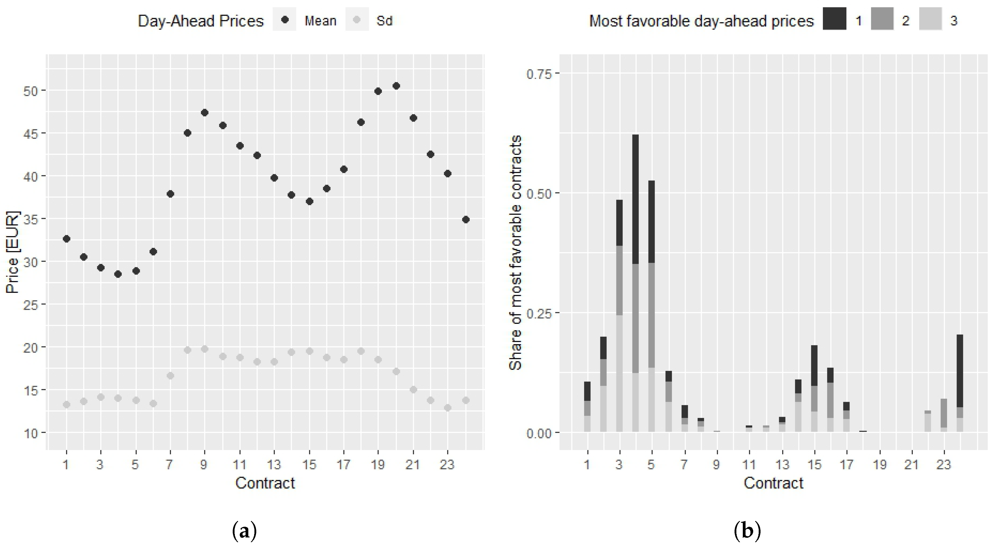
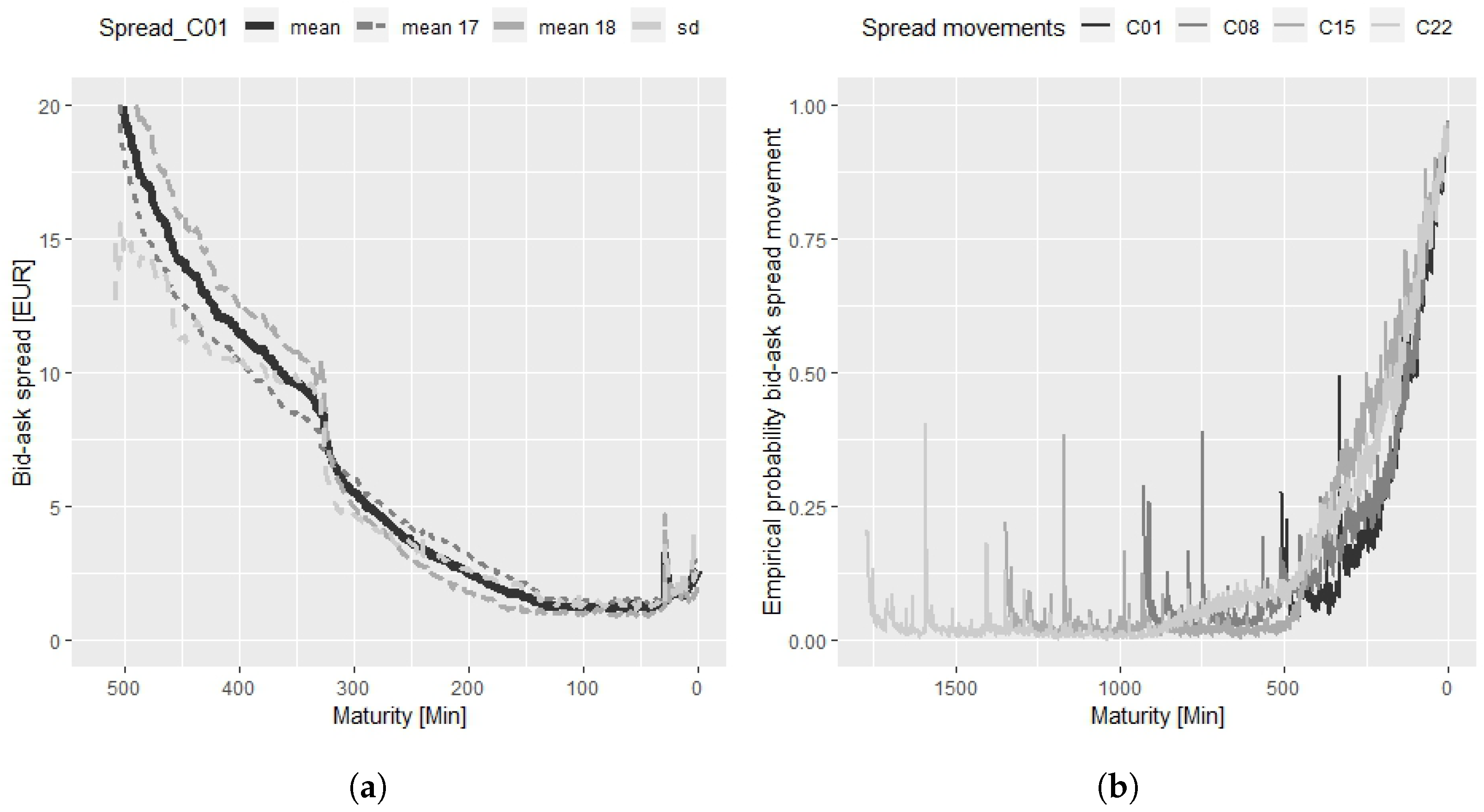
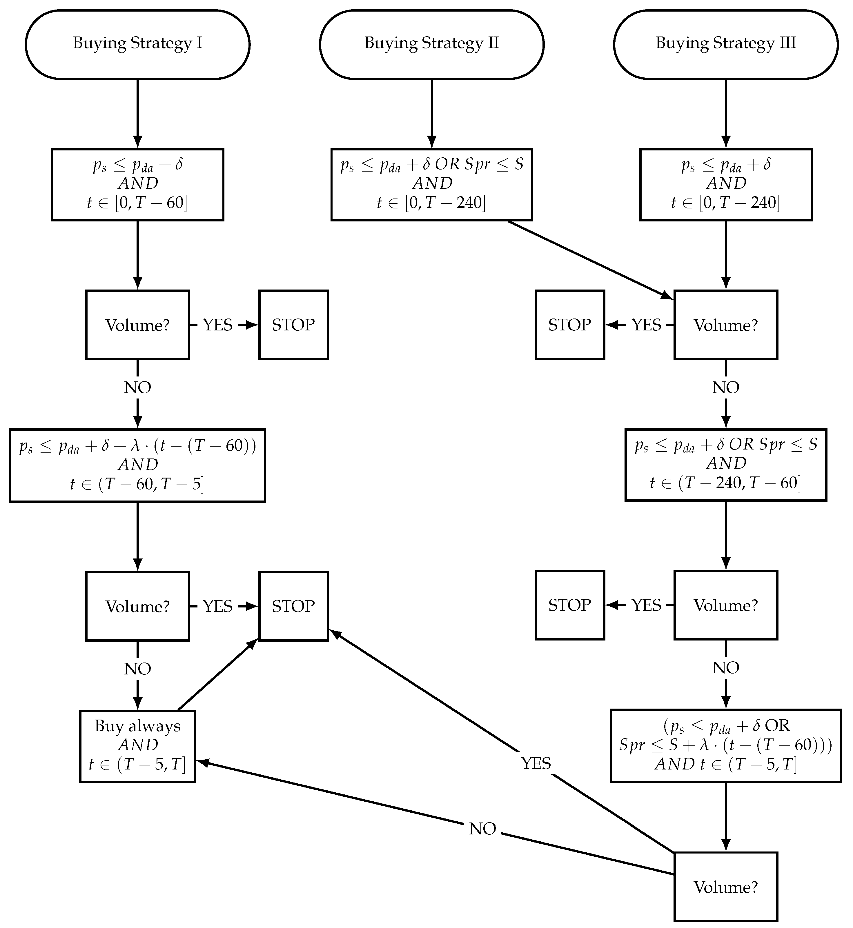
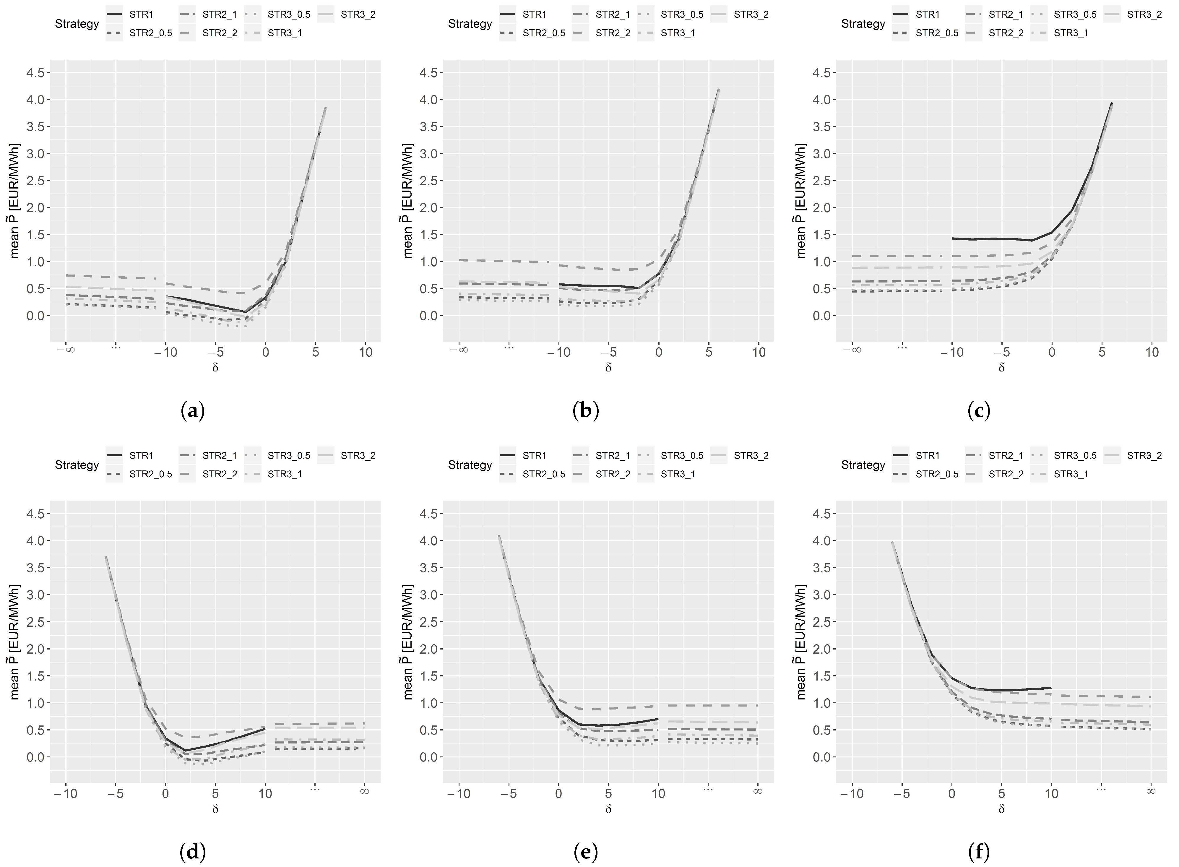
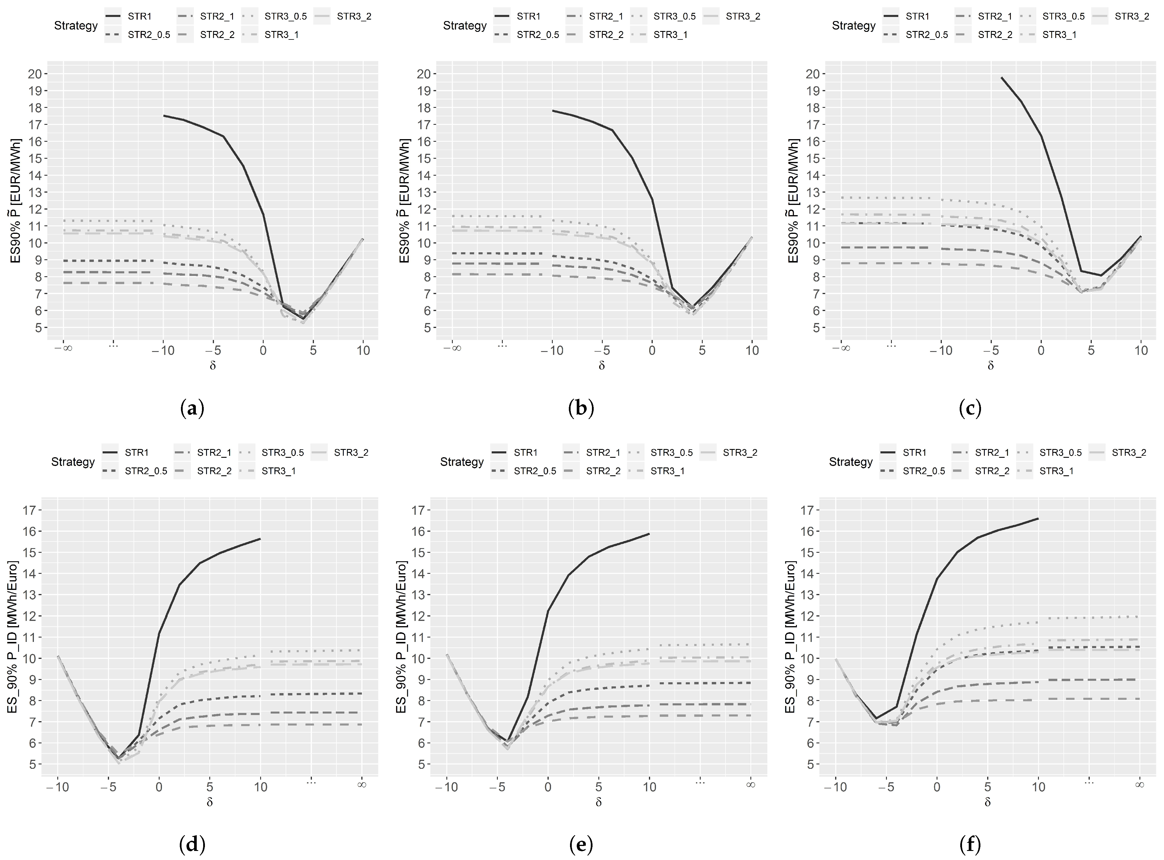
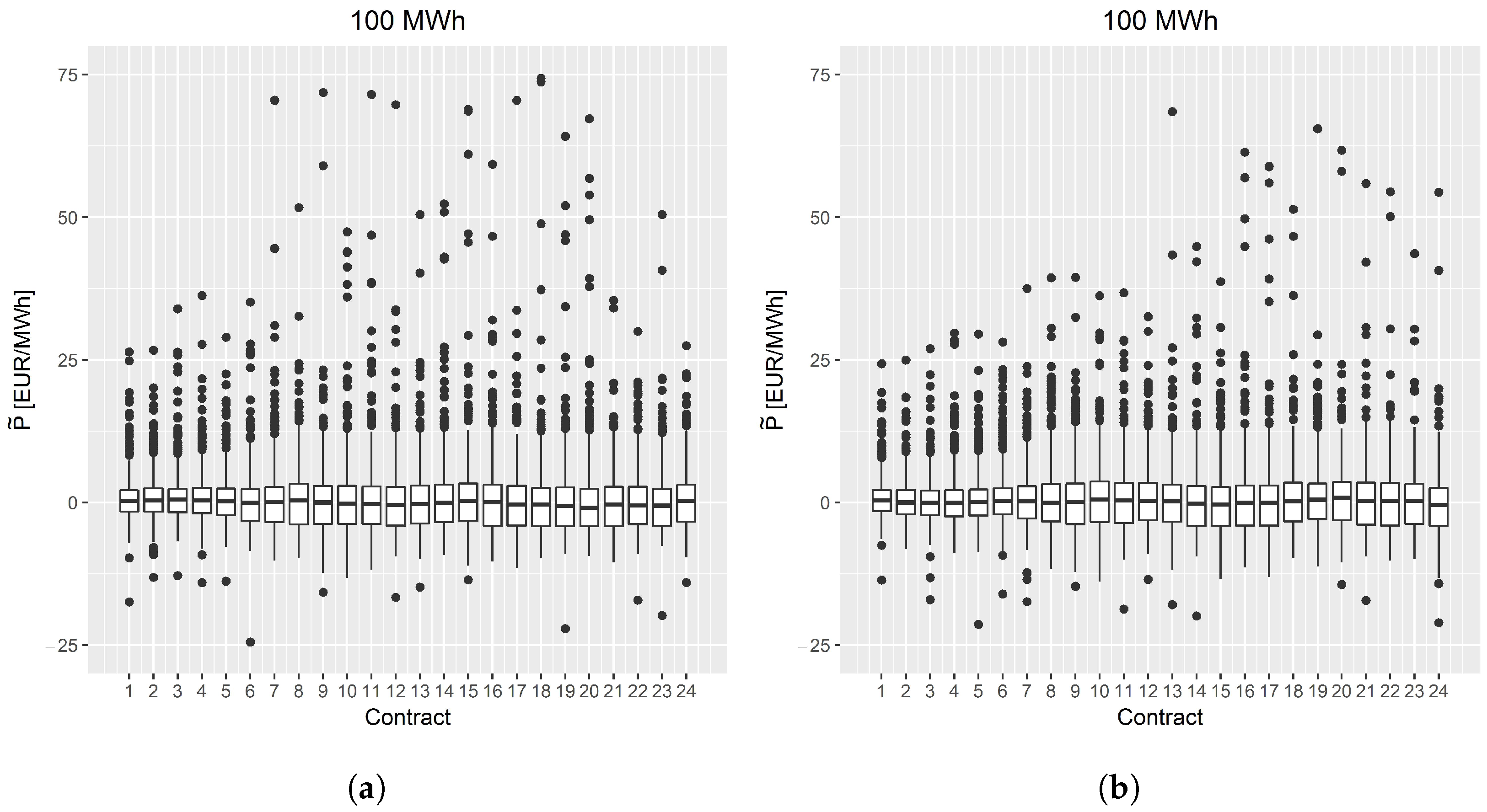
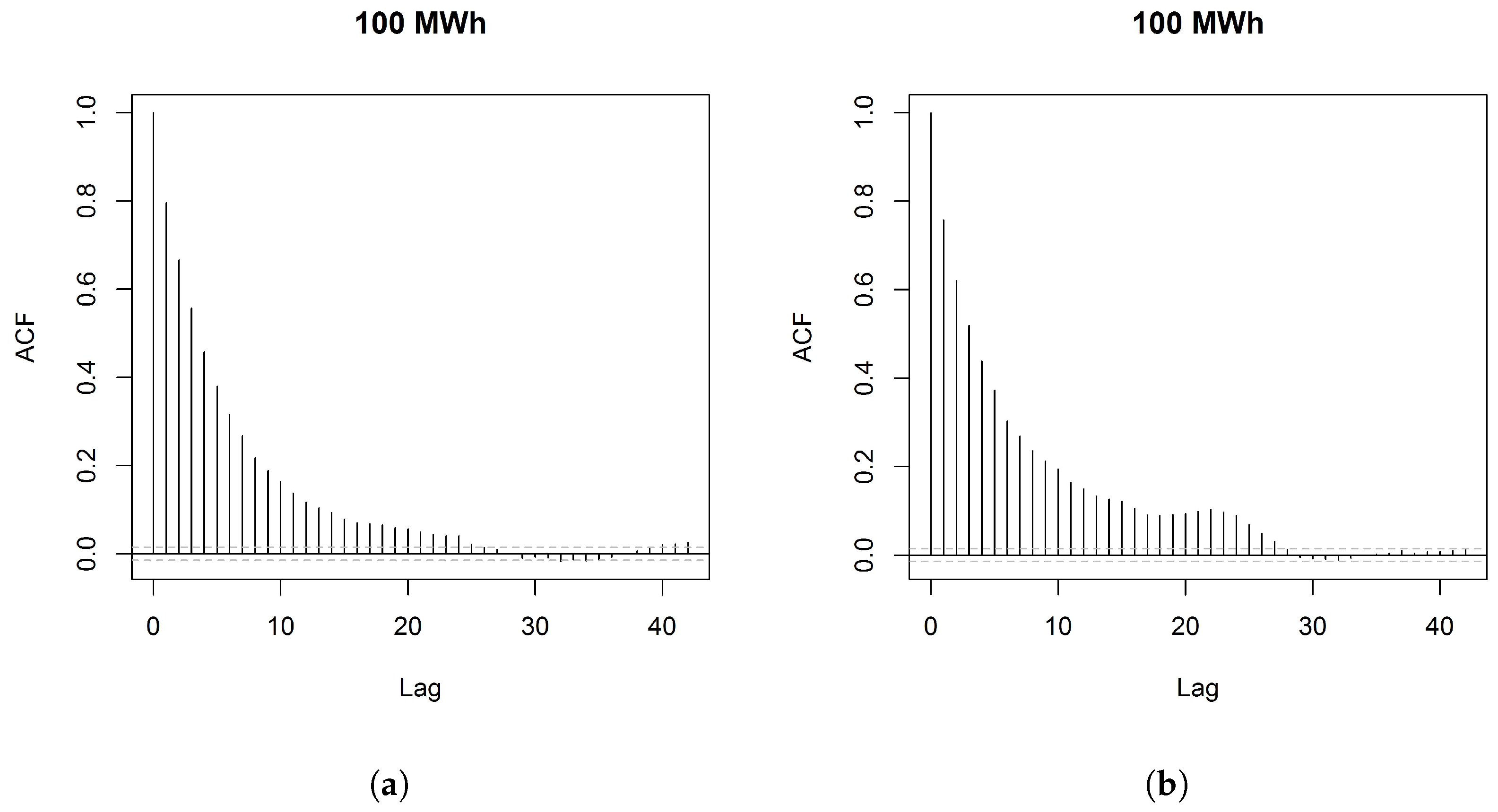
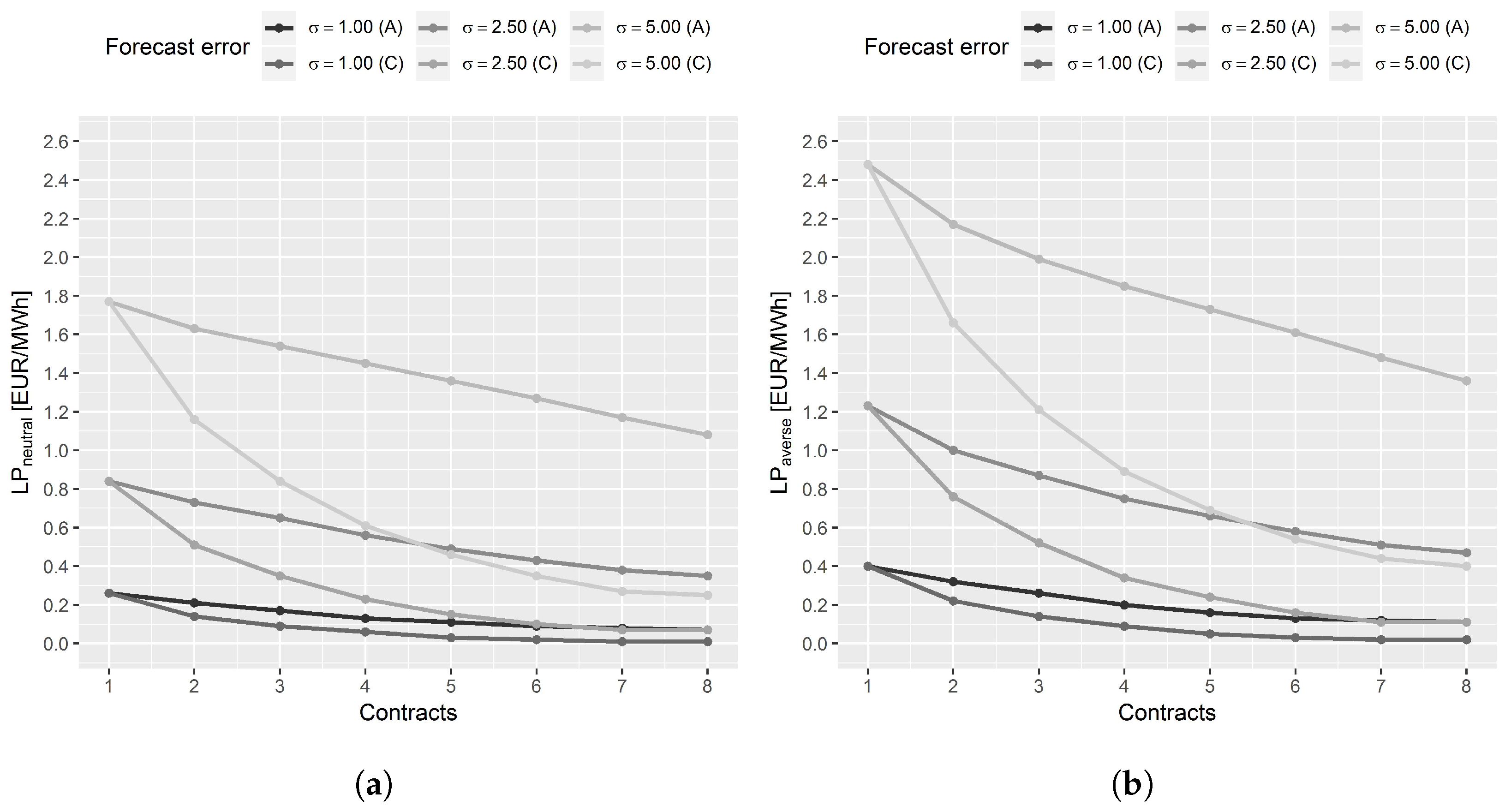
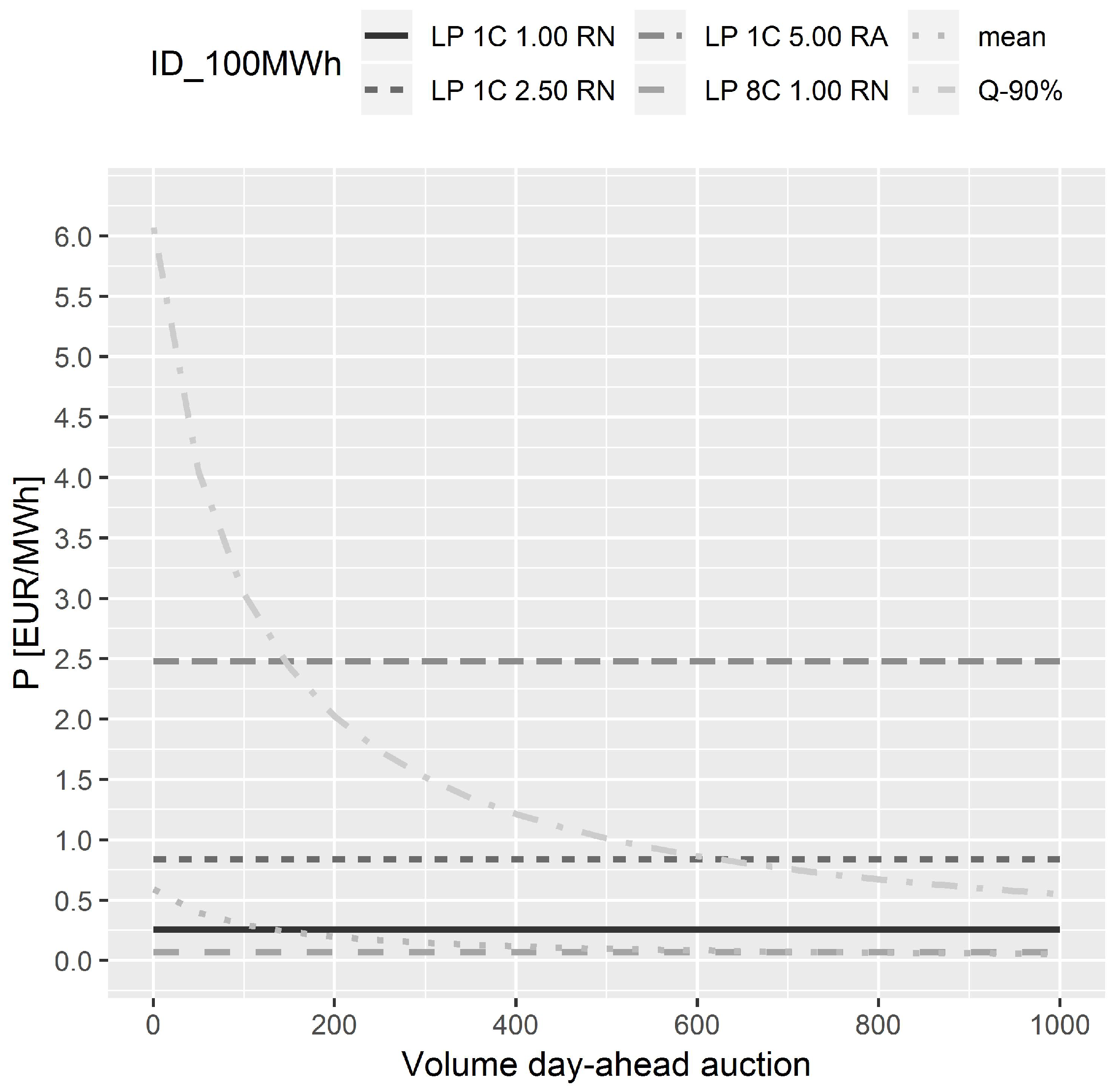
Table 1.
Descriptive statistics of the continuous intraday order book. The statistics include information on the number of buy orders, volume of buy orders, volume-weighted average price of buy orders, number of sell orders, volume of sell orders, volume-weighted average price of sell orders, the volume actually traded (national), and the number of hourly contracts observed. The results are presented for the different quarters of 2017 and 2018 and in total. Orders with the same OrderID due to partial executions were only considered once.
| 2017 | 2018 | Total | |||||||
|---|---|---|---|---|---|---|---|---|---|
| Q1 | Q2 | Q3 | Q4 | Q1 | Q2 | Q3 | Q4 | ||
| # Buy (Mio.) | 3.15 | 3.03 | 2.96 | 3.58 | 4.31 | 4.77 | 5.16 | 7.49 | 34.45 |
| Vol. Buy (TWh) | 40.61 | 34.00 | 34.67 | 42.06 | 43.82 | 45.11 | 40.14 | 50.70 | 331.11 |
| Buy (EUR) | 29.32 | 20.35 | 20.44 | 14.82 | 28.79 | 23.59 | 30.54 | 14.14 | 22.74 |
| # Sell (Mio) | 2.46 | 2.41 | 2.62 | 3.22 | 3.88 | 4.34 | 4.78 | 7.65 | 31.37 |
| Vol. Sell (TWh) | 31.66 | 27.43 | 30.13 | 36.64 | 37.87 | 40.37 | 36.30 | 50.04 | 290.43 |
| Sell (EUR) | 58.82 | 40.70 | 45.66 | 56.85 | 44.78 | 49.23 | 93.92 | 94.58 | 60.53 |
| Tr. Vol. (TWh) | 7.55 | 7.52 | 7.33 | 7.65 | 7.97 | 8.58 | 7.88 | 8.10 | 62.57 |
| # Contracts | 2073 | 2158 | 2176 | 2114 | 2066 | 2119 | 2159 | 2085 | 16,950 |
Table 2.
Descriptive statistics for strategy premiums for Strategy III with a volume of 100 MWh, separated into buying and selling strategies for different and different S.
Table 2.
Descriptive statistics for strategy premiums for Strategy III with a volume of 100 MWh, separated into buying and selling strategies for different and different S.
| Buying Strategy | Selling Strategy | ||||||||||
|---|---|---|---|---|---|---|---|---|---|---|---|
| Panel A: Strategy III with | |||||||||||
| min | −47.92 | −24.46 | −26.03 | −26.12 | −25.33 | −17.29 | −21.36 | −21.36 | −23.47 | −48.29 | |
| median | 0.28 | 0.25 | −0.01 | −0.28 | 2.59 | 2.69 | −0.24 | 0.14 | 0.38 | 0.44 | |
| mean | 0.48 | 0.50 | 0.59 | 1.07 | 2.66 | 2.72 | 1.16 | 0.67 | 0.57 | 0.51 | |
| max | 182.84 | 182.84 | 182.84 | 154.13 | 122.36 | 84.52 | 84.52 | 84.52 | 84.52 | 84.52 | |
| sd | 7.19 | 6.78 | 6.23 | 4.99 | 3.44 | 2.86 | 4.24 | 5.28 | 5.88 | 6.62 | |
| skewness | 4.15 | 5.59 | 7.21 | 8.92 | 14.20 | 8.98 | 4.87 | 2.78 | 1.81 | 0.10 | |
| kurtosis | 78.63 | 95.74 | 131.31 | 156.83 | 341.04 | 158.75 | 48.42 | 21.67 | 14.98 | 16.52 | |
| 12.68 | 12.55 | 12.20 | 10.96 | 7.21 | 7.09 | 10.44 | 11.37 | 11.70 | 11.96 | ||
| Panel B: Strategy III with | |||||||||||
| min | −45.33 | −26.03 | −26.03 | −26.12 | −25.33 | −17.29 | −21.36 | −21.36 | −23.47 | −48.23 | |
| median | 0.43 | 0.40 | 0.22 | −0.25 | 2.59 | 2.69 | −0.21 | 0.36 | 0.52 | 0.56 | |
| mean | 0.56 | 0.58 | 0.67 | 1.08 | 2.65 | 2.71 | 1.17 | 0.74 | 0.66 | 0.60 | |
| max | 160.04 | 160.04 | 160.04 | 160.04 | 118.79 | 74.49 | 74.49 | 74.49 | 74.49 | 74.49 | |
| sd | 6.65 | 6.30 | 5.82 | 4.69 | 3.24 | 2.75 | 3.97 | 4.89 | 5.41 | 6.09 | |
| skewness | 4.35 | 5.74 | 7.23 | 8.94 | 13.27 | 8.87 | 4.64 | 2.57 | 1.66 | −0.12 | |
| kurtosis | 85.41 | 102.18 | 135.61 | 171.07 | 310.02 | 161.58 | 48.27 | 21.63 | 15.51 | 18.39 | |
| 11.68 | 11.57 | 11.32 | 10.30 | 7.10 | 7.01 | 9.75 | 10.43 | 10.69 | 10.89 | ||
| Panel C: Strategy III with | |||||||||||
| min | −43.55 | −24.46 | −24.46 | −24.46 | −22.83 | −17.29 | −21.36 | −21.36 | −23.47 | −48.23 | |
| median | 0.77 | 0.75 | 0.62 | −0.21 | 2.59 | 2.69 | −0.16 | 0.79 | 0.90 | 0.92 | |
| mean | 0.88 | 0.89 | 0.92 | 1.18 | 2.65 | 2.72 | 1.30 | 1.02 | 0.99 | 0.94 | |
| max | 155.29 | 155.29 | 155.29 | 105.20 | 91.00 | 68.07 | 68.07 | 68.07 | 68.07 | 68.07 | |
| sd | 6.02 | 5.77 | 5.37 | 4.32 | 2.98 | 2.58 | 3.81 | 4.65 | 5.06 | 5.64 | |
| skewness | 3.42 | 4.50 | 5.51 | 6.60 | 10.58 | 7.15 | 3.71 | 1.98 | 1.18 | −0.53 | |
| kurtosis | 65.10 | 73.64 | 92.45 | 96.06 | 212.19 | 123.47 | 34.49 | 15.84 | 12.04 | 17.89 | |
| 11.15 | 11.10 | 10.92 | 10.00 | 7.10 | 7.05 | 9.58 | 10.11 | 10.29 | 10.40 | ||
Table 3.
Strategy premiums by subset (mean and quantiles) for separate buying or selling strategies. Premiums are based on Strategy III, and . Panel A distinguishes between the two years 2017 and 2018. In Panel B, subsets of realized strategy premiums are formed according to the daily realized prices of the day-ahead auction. Thus, the contracts of the day-ahead auction are sorted by their prices on a daily basis, and the subsets contain the corresponding strategy premiums separated by the cheapest and most-expensive daily contracts. In addition, a subset was provided containing all strategy premiums associated with the day-ahead contracts that achieved a negative price.
| Buying Strategy | Selling Strategy | ||||||
|---|---|---|---|---|---|---|---|
| Mean | 90% | 95% | Mean | 90% | 95% | ||
| Panel A: Years | |||||||
| 2017 | 0.63 | 6.08 | 8.95 | 0.95 | 6.70 | 9.89 | 8521 |
| 2018 | 0.55 | 6.06 | 8.76 | 0.38 | 5.75 | 8.29 | 8429 |
| Panel B: Day-ahead auction prices | |||||||
| lowest | 1.88 | 8.18 | 11.95 | −0.35 | 4.69 | 8.71 | 707 |
| 2 lowest | 1.58 | 7.57 | 11.53 | −0.11 | 4.90 | 8.28 | 1417 |
| 3 lowest | 1.34 | 7.16 | 10.72 | −0.05 | 4.90 | 8.32 | 2118 |
| 4 lowest | 1.18 | 6.69 | 10.18 | 0.09 | 5.11 | 8.40 | 2821 |
| 5 lowest | 1.08 | 6.31 | 10.00 | 0.21 | 5.18 | 8.50 | 3513 |
| 6 lowest | 0.96 | 6.23 | 9.65 | 0.33 | 5.39 | 8.74 | 4220 |
| highest | −0.19 | 5.59 | 8.19 | 1.83 | 7.97 | 11.86 | 717 |
| 2 highest | −0.02 | 5.57 | 8.33 | 1.52 | 7.64 | 11.35 | 1426 |
| 3 highest | 0.03 | 5.56 | 8.34 | 1.45 | 7.43 | 10.82 | 2141 |
| 4 highest | 0.13 | 5.58 | 8.19 | 1.36 | 7.34 | 10.36 | 2851 |
| 5 highest | 0.15 | 5.59 | 8.11 | 1.24 | 7.27 | 9.96 | 3547 |
| 6 highest | 0.16 | 5.69 | 8.17 | 1.20 | 7.14 | 9.81 | 4267 |
| 8.77 | 27.39 | 36.25 | −2.33 | 5.47 | 18.69 | 254 | |
Table 4.
Descriptive statistics of the explanatory variables. is the difference between realized wind energy and forecast wind energy in GWh; is the relative wind share of total consumption. and are analogously defined as the difference between realized solar energy in GWh and forecast solar energy, respectively. is the difference between realized other energies and forecast other energies in GWh, and is the difference between realized consumption and forecast consumption in GWh.
| min | −9.697 | −4.698 | −24.00 | −15.84 | 0.003 | 0.000 |
| 25% | −0.597 | −0.019 | −8.249 | −0.248 | 0.089 | 0.000 |
| median | 0.047 | 0.000 | −4.823 | 0.970 | 0.175 | 0.002 |
| mean | 0.138 | 0.004 | −5.381 | 1.081 | 0.214 | 0.072 |
| 75% | 0.841 | 0.008 | −2.217 | 2.351 | 0.306 | 0.113 |
| max | 10.78 | 4.662 | 19.42 | 10.26 | 0.848 | 0.584 |
| sd | 1.434 | 0.669 | 4.680 | 2.006 | 0.157 | 0.112 |
Table 5.
Regression results for Strategy III, and , for different volumes. The coefficients of the explanatory variables, the adjusted , and the number of observations are given. is the difference between realized and forecast wind energy in GWh; is the relative wind share of the total consumption. , , and are analogously defined for solar energy and other energy, respectively. is the difference between realized consumption and forecast consumption in GWh. The asterisks denote the significance level, with *** = 0.1%, ** = 1%, and * = 5%.
| Panel A: Buying Strategy | Panel B: Selling Strategy | |||||
|---|---|---|---|---|---|---|
| 0.1 MWh | 10 MWh | 100 MWh | 0.1 MWh | 10 MWh | 100 MWh | |
| −1.878 ** | −1.287 * | −1.178 | 0.348 | 1.148 * | 1.575 ** | |
| (0.642) | (0.632) | (0.644) | (0.541) | (0.49) | (0.497) | |
| −1.152 *** | −1.234 *** | −1.477 *** | 1.143 *** | 1.217 *** | 1.410 *** | |
| (0.088) | (0.085) | (0.079) | (0.074) | (0.069) | (0.069) | |
| −0.948 *** | -0.942 *** | −1.210 *** | 0.892 *** | 0.936 *** | 1.192 *** | |
| (0.116) | (0.115) | (0.13) | (0.119) | (0.116) | (0.112) | |
| 0.024 | 0.001 | 0.004 | −0.046 | −0.032 | −0.007 | |
| (0.036) | (0.035) | (0.038) | (0.038) | (0.035) | (0.035) | |
| 0.234 *** | 0.263 *** | 0.299 *** | −0.184 ** | −0.235 *** | −0.255*** | |
| (0.052) | (0.052) | (0.054) | (0.063) | (0.061) | (0.058) | |
| 2.424 * | 2.327 * | 3.356 ** | −2.223 * | −1.494 | −0.919 | |
| (1.13) | (1.13) | (1.214) | (1.006) | (0.984) | (1.08) | |
| 2.715 | 2.345 | 2.445 | −5.226 ** | −4.195 * | −2.05 | |
| (1.58) | (1.51) | (1.681) | (1.717) | (1.697) | (1.788) | |
| fixed effects | yes | yes | yes | yes | yes | yes |
| adj. | 0.092 | 0.111 | 0.154 | 0.120 | 0.144 | 0.184 |
| Observations | 16,631 | 16,631 | 16,631 | 16,631 | 16,631 | 16,631 |
Publisher’s Note: MDPI stays neutral with regard to jurisdictional claims in published maps and institutional affiliations. |
© 2022 by the authors. Licensee MDPI, Basel, Switzerland. This article is an open access article distributed under the terms and conditions of the Creative Commons Attribution (CC BY) license (https://creativecommons.org/licenses/by/4.0/).
Share and Cite
MDPI and ACS Style
Baule, R.; Naumann, M. Flexible Short-Term Electricity Certificates—An Analysis of Trading Strategies on the Continuous Intraday Market. Energies 2022, 15, 6344. https://doi.org/10.3390/en15176344
AMA Style
Baule R, Naumann M. Flexible Short-Term Electricity Certificates—An Analysis of Trading Strategies on the Continuous Intraday Market. Energies. 2022; 15(17):6344. https://doi.org/10.3390/en15176344
Chicago/Turabian StyleBaule, Rainer, and Michael Naumann. 2022. "Flexible Short-Term Electricity Certificates—An Analysis of Trading Strategies on the Continuous Intraday Market" Energies 15, no. 17: 6344. https://doi.org/10.3390/en15176344
Note that from the first issue of 2016, this journal uses article numbers instead of page numbers. See further details here.