
Profitability and Revenue Uncertainty of Wind Farms in Western Europe in Present and Future Climate
by
 and
and
Bastien Alonzo
1,
Silvia Concettini
2,3,
Anna Creti
2,4,
Philippe Drobinski
1 and
Peter Tankov
5,* 1
Laboratoire de Météorologie Dynamique-Institut Pierre-Simon Laplace, Ecole Polytechnique, Institut Polytechnique de Paris, Ecole Normale Supérieure (ENS), Paris Sciences Lettres Research University, Sorbonne Université, Centre National de Recherche Scientifique, 91120 Palaiseau, France
2
Climate Economics Chair, 75002 Paris, France
3
Energy and Prosperity Chair, 75002 Paris, France
4
Centre de Géopolitique de L’énergie et des Matières Premières, Paris Dauphine-Paris Sciences Lettres University, 75016 Paris, France
5
Centre de Recherche en Economie et Statistique, Ecole Nationale de Statistique et Administration Economique, Institut Polytechnique de Paris, 91120 Palaiseau, France
*
Author to whom correspondence should be addressed.
Energies 2022, 15(17), 6446; https://doi.org/10.3390/en15176446
Submission received: 9 August 2022
/
Revised: 28 August 2022
/
Accepted: 29 August 2022
/
Published: 3 September 2022
(This article belongs to the Special Issue Technical and Economic Analysis of Electricity Markets)
Abstract
:Investments into wind power generation may be hampered by the uncertainty of future revenues caused by the natural variability of the wind resource, the impact of climate change on wind potential and future electricity prices, and the regulatory risks. We quantify the uncertainty of the economic value of wind farms in France, Germany, and Denmark, and evaluate the cost of support mechanisms needed to ensure the profitability of wind farms under present and future climates. To this end, we built a localised model for wind power output and a country-level model for electricity demand and prices. Our study reveals that support mechanisms are needed for current market conditions and the current climate, as well as under future climate conditions according to several scenarios for climate change and energy transition. The cost of support mechanisms during a 15-year period is evaluated to EUR 3.8 to EUR 11.5 billion per year in France, from EUR 15.5 to EUR 26.5 billion per year in Germany, and from EUR 1.2 to EUR 3.3 billion per year in Denmark, depending on the scenario considered and the level of penetration of wind energy.
1. Introduction
To limit greenhouse gas emissions from power generation, as well as the dependence on energy imports, the use of renewable intermittent energy sources, such as wind and solar, has been encouraged in many European countries. Renewable energy generation, together with the electrification of carbon-intensive sectors, such as transport and heating, are the pillars of energy transition. In this context, wind energy plays a particularly important role because of high wind potential in Europe, rapidly decreasing costs of technology, regulated support mechanisms, and good acceptance by the public. In 2021, EUR 41 billion was spent on building new wind power plants in Europe, for a record total of 24.6 GW of new capacity, and this figure is expected to increase in the short term due to favourable economic conditions, policy initiatives, such as the European Green Deal, and the necessity to reduce dependence on the Russian gas exports in the current political context [1]. However, this still falls short of the declared energy transition objectives: in its REPowerEU roadmap the European Commission has fixed a new objective of 480 GW of installed wind power capacity in the EU by 2030 to reduce energy prices and enhance energy security. This requires the addition of 35 GW of wind capacity annually between 2022 and 2030.
The investment into wind energy production is hampered by the uncertainty of future revenues of wind power producers. This uncertainty arises from the natural variability of the resource, from climate change, which is likely to impact not only future wind energy production but also electricity prices and, last but not least, from the evolution of regulatory policies. A more precise understanding of the uncertainties at stake is, therefore, needed for a number of reasons. First, it will give the private sector investors a better view of risks and opportunities associated with wind energy industry. Second, it will enable the public authorities to quantify the level of support needed for long-term sustainability of the industry and to evaluate the long term costs of energy transition. Finally, it will allow the financial industry to develop suitable funding instruments.
The potential for future cost reduction in wind energy production is analysed in several recent articles. In [2], the authors summarise the results of a global expert survey of wind energy costs; they anticipate a 24–30% cost reduction by 2030 and a 35–41% reduction by 2050. Another recent article [3] also predicts a drop of 40% by 2050 in capital costs for onshore wind turbines. The articles [4,5] study the evolution of levelized cost of wind generated electricity, both anticipating cost reductions for this generation technology. The paper [6] identifies four main drivers for past cost changes: learning by deployment, learning by researching, supply chain dynamics, and market dynamics, including support policies. In [7], the authors study the impact of sector coupling on the cost of energy system development in Northern–Central Europe using the Balmorel energy system model [8], and in [9] the costs of increasing renewable energy penetration in the US are explored in the framework of the Regional Energy Deployment System (ReEDS) model [10]. When it comes to the value of wind power plants, several studies agree that it tends to decline as penetration rate increases [11,12,13]. A full model for the economic value of wind at increasing penetration taking into account hourly variation of wind and load is presented in [14]. An interesting model recently proposed in [15] analyses the effects of strategic behaviour of wind producers and heterogeneous resource availability.
Concerning support policies, real-options models with stochastic dynamics are developed in [16,17] to compare the costs of different policy schemes. Scenarios for future worldwide wind power deployment, associated costs, and policy options are reviewed in [18], while the papers [19,20] discuss the risks and risk management options of renewable energy projects, in particular revenue variability risks associated to resource intermittency and price volatility, that we also address in this paper. The article [21] evaluates the wind and solar subsidies in Spain and in Germany in terms of their cost for reducing carbon emissions and find that it is much cheaper for the regulator to reduce CO emissions by subsidizing the wind power production. At the same time, the paper [22] finds that wind subsidies in Germany may not be fully efficient since, in addition to helping wind producers, they also push land prices up, creating windfall revenues for land owners. Finally, a very recent preprint [23] considers optimal structuring of renewable energy subsidies taking into account the learning curves.
Regarding the impact of climate change on wind speed, the article [24] studies its consequences on the optimal power generation and transmission expansion plan in Chile. Some articles use reanalysis data to quantify wind potential and assess its uncertainty, see, e.g., [25]. The impact of climate change on wind potential and levelized cost of wind energy is analysed in [26,27] using CMIP5 scenarios. However, these papers, which use climate data to evaluate the wind potential, do not combine it with the price and electricity demand component. This is all the more important because the impact of climate change on electricity demand, due, in particular, to the global temperature change, is expected to be stronger than the impact on the wind potential [28]. The economics of wind energy is studied only in terms of costs but not in terms of actual revenues for the wind producers operating in the market, and, consequently, the cost of public support measures needed to make wind energy profitable is rarely evaluated.
We propose to fill this gap by quantifying the uncertainty of the net present value of standardized wind farms in European countries and by evaluating the level and the total cost of support mechanisms needed to guarantee the profitability of the wind fleet. To this end, we build a localized model for wind power output and a country-level model for electricity demand and prices taking into account hourly variation of wind, load and prices, using reanalysis data, climate projections, and integrated assessment model (IAM) scenarios. The main focus of our study is to quantify the uncertainty due to climate variability and climate change. Our model for the electricity demand is thus relatively simple compared to the literature, but allows to quantify the climate impacts very precisely. We develop a general methodology, focusing on the examples of France, Germany, and Denmark for specific evaluations. Our study shows that profitability of wind energy in these countries requires support mechanisms under current market prices and current climate. We then analyse several scenarios of climate change and energy transition, and show that, under future climate, support mechanisms will still be needed in these countries to ensure the economic sustainability of the wind energy.
The rest of the paper is structured as follows. In Section 2, we briefly describe the model that we use to generate long time series of synthetic electricity prices and wind energy output under present and future climate. In Section 3, we analyse the variability of wind farm revenues and value under present climate. Section 4 presents the analysis of wind farm value under future climate and various socio-economic scenarios. In this section we also evaluate the cost of public support schemes required to ensure the economic sustainability of wind energy in the future. Section 5 places our results in a wider context and discusses their policy implications, and Section 6 concludes the paper. A list of frequently used abbreviations is provided after this section.
2. Modelling Electricity Prices and Local Wind Production
Our methodology relies on constructing a long time series of synthetic local wind power production and national electricity prices, built assuming current market conditions. This is done by plugging a long time series of climate variables into a model for wind power production and for electricity prices, calibrated on recent market and energy system data. The time series of climate variables are obtained either from historical reanalysis data (for current climate analysis) or from regional climate model projections (for future climate analysis). The synthetic local wind power production and national electricity prices are then used to simulate the revenues of standardized wind farms depending on their location, under different scenarios. This approach allows to disentangle the different sources of variability and to quantify the variations in the revenues and expenditure of wind farms at current market design and network structure, under different support schemes.
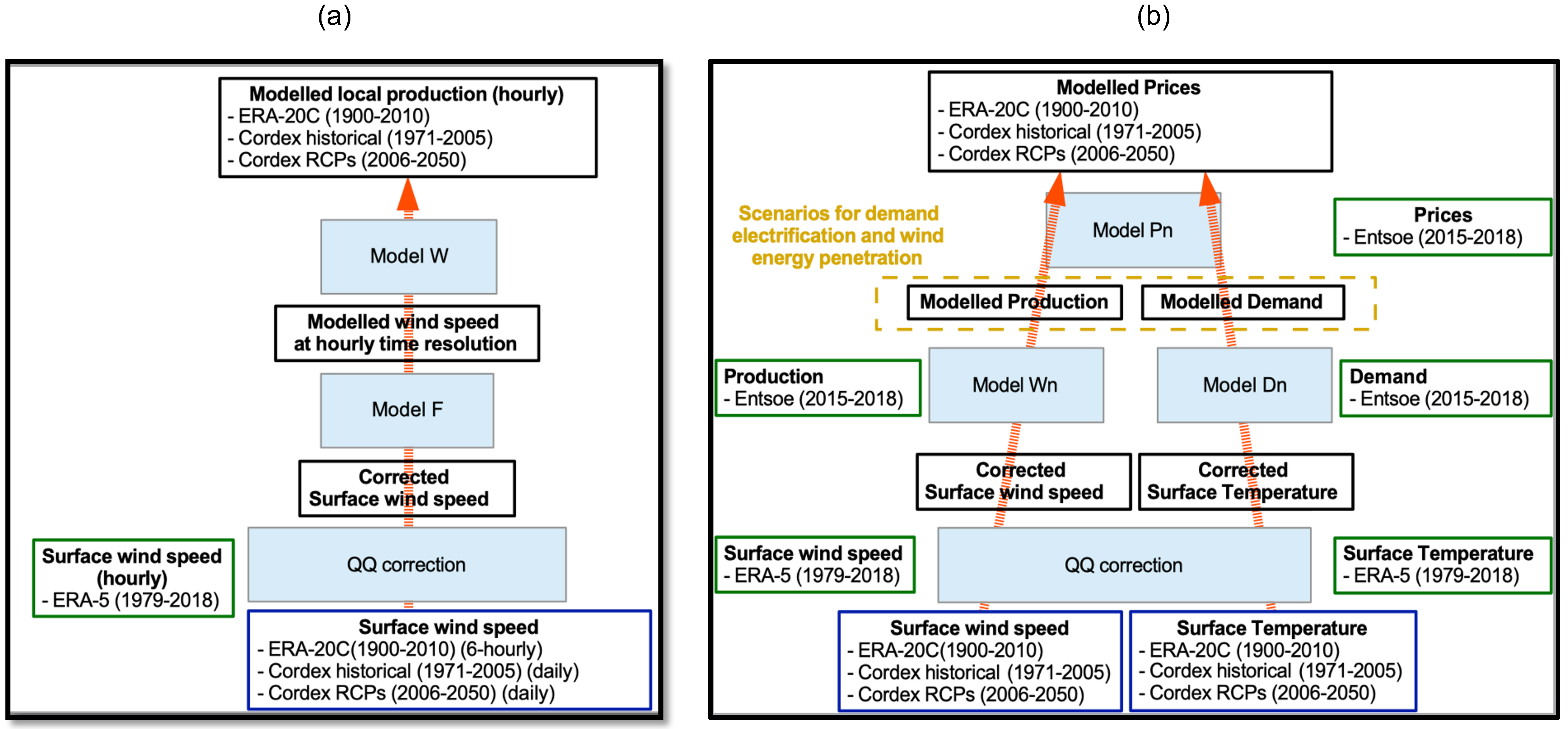
Here, we briefly describe the modelling approach to generate the time series. A summary of the variables and the data sources is provided in the Data section in the Appendix A and a detailed description of the modelling approach is presented in the Models section of the same appendix. Figure 1 presents the modelling process for wind energy infeed at each gridpoint of the considered domain (Figure 1a) and for day-ahead prices in each of the three considered countries (Figure 1b). Both models have three steps, going from the bottom to the top of Figure 1.
In the first step, which is common to the two models, we reduce the bias of the long time series of surface wind speed and temperature from the ERA20C reanalysis by comparing them to the ERA-5 reanalysis dataset, which is considered to be more reliable and less biased, and performing a quantile-quantile correction. Recall that reanalysis is a procedure wherein a single model for the atmosphere is run over an extended historical period, coupled with an assimilation system, which assimilates all available observations for this period. This results in a long homogeneous time series of the evolution of the atmosphere which represents our best guess of the state of the atmosphere given the available data. For the local production model, in the second modelling step, we downscale the wind speed time series to hourly frequency by generating the missing values from a stochastic wind model. In the third step, we combine the local wind speed with standardized production functions to obtain a time series of the synthetic local wind power production. For the price model, the second step consists in generating long time series of national production and demand, using models whose parameters are estimated from historical data from a recent period. The third step allows to obtain a time series of synthetic prices from the generated production and demand values.
As a result of these modelling processes, we obtain two datasets:
- The present climate dataset used to study the variability of wind farm revenues and value at current climate, i.e., at 20th century climate variability but with current market and energy system characteristics;
- The future climate dataset used to study the variability of the wind farm revenues and value under future climate and future realistic scenarios for demand and wind energy penetration, taking into account the climate model uncertainty.
We now proceed to describe the two datasets in detail. The present climate dataset contains synthetic local wind power production data at the spatial resolution of and synthetic day-ahead prices, electricity demand, and national wind energy production in France, Germany, and Denmark. All series have hourly time resolution and correspond to the climate data from 1900 to 2010.
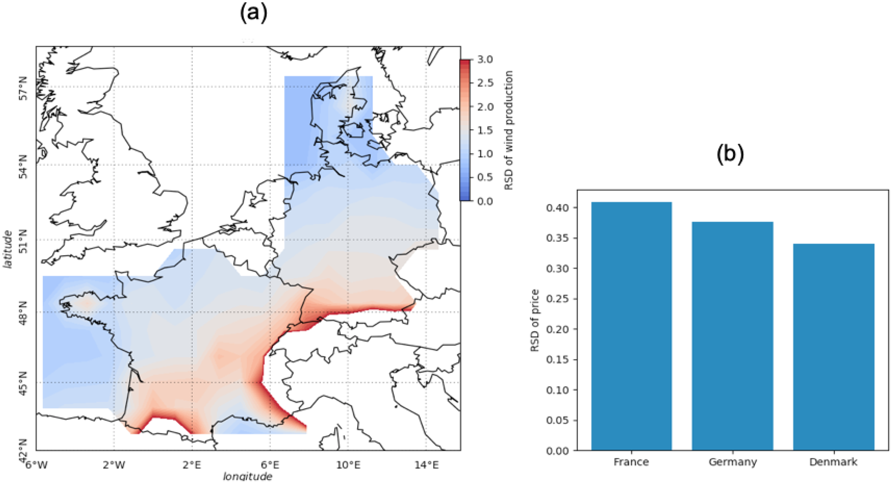
This dataset is illustrated in Figure 2, Figure 3 and Figure 4. Figure 2 displays the relative standard deviation (i.e., the ratio between the standard deviation and the mean, henceforth RSD) of onshore and offshore production capacity factor in panel (a), and of price in panel (b) for each considered country. It is clear that the variability of revenues is largely explained by that of the capacity factor, which is much more variable than the price in all countries under consideration. The standard deviation of the price is around 35% of the mean price, while the standard deviation of the capacity factor exceeds the mean capacity factor in most onshore regions, especially in locations where the mean capacity factor is low (e.g., mountainous regions). In France, the price RSD exceeds 45% because the seasonal cycle is more pronounced than in the other countries due to strong seasonal variations of the consumption.
At the hourly timescale (panel (c)), the correlation between prices and production is low but positive (<0.2). At the monthly timescale (panel (d)), wind energy production is significantly positively correlated with prices in all three countries under study. This is due to matching seasonal cycles of wind energy production and prices. Indeed, prices are high during cold seasons when demand increases. At the same time, wind production in Western Europe is also expected to be high during the cold season due to the enhanced activity of the storm track. In the long term (panel (e)), the correlation between wind energy production and prices becomes negative, especially in Denmark and the north of Germany. This may be related to the merit-order effect: a rise in wind production at the national level tends to push the wholesale electricity price down (see [29,30] for instance). It may also indicate a negative correlation between temperature (whose increase tends to push the demand and thus the prices down) and wind energy production. This correlation can also be related to the large scale weather regimes, such as the North Atlantic Oscillation (NAO) which, in the positive phase, enhances the storm track activity, increasing the wind production in Western Europe, and, at the same time, contributes to increasing the temperature and, therefore, decreasing energy demand and prices, by bringing warmer wet air in this region. In the negative phase, this phenomenon is reversed. The NAO displays long term cycles of the order of 3 to 7 years. Many studies have demonstrated a correlation of the NAO (and other weather regimes) with wind speed and production and electricity demand (see for instance [31,32]).
Figure 3 shows the correlation between synthetic prices and production at different timescales.
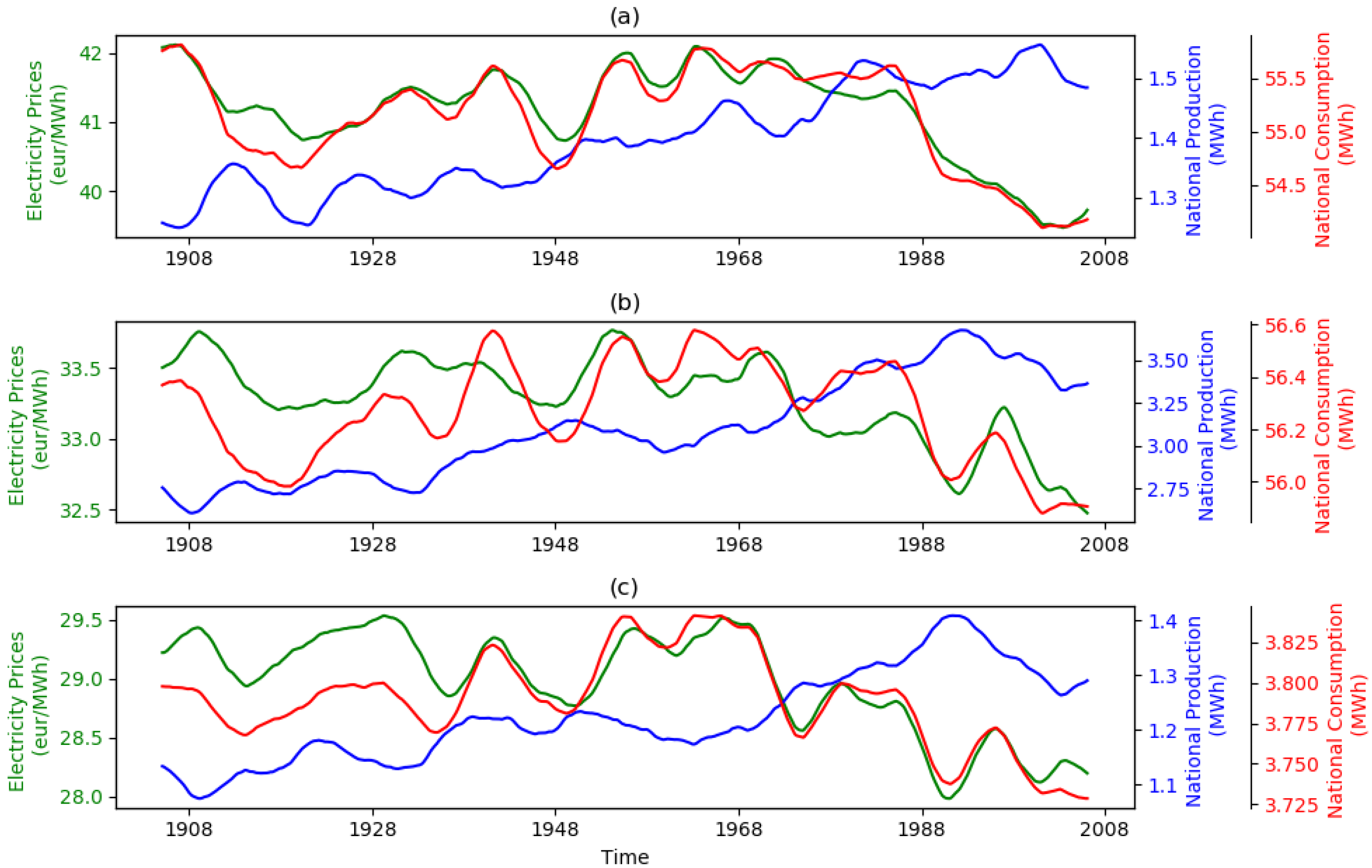
Figure 4 displays the long-term trends (10 years sliding mean) of the synthetic electricity prices, electricity consumption, and wind energy production in France, Germany, and Denmark (Figure 4a–c, respectively). As expected from our model, where the electricity prices are largely driven by consumption, these two time series tend to vary together. On the other hand, the negative correlations between electricity prices and wind energy production, discussed above, are not clearly visible on this graph due to averaging. We observe long-term trends in consumption and price trajectories, especially after the late 1960s when they both decrease, and very long-term trends in wind energy production, which increases in all three countries throughout the 20th century and appears to decrease afterwards. The authors of [33] identify such positive trends for wind speed in ERA20C, CERA20C reanalyses, as well as in the OFA observation dataset (assimilated in these reanalyses). They also identify negative trends in NOAA20CR reanalysis, and no trends in the free simulation ERA20CM which uses the same model as ERA20C. The study focuses on North Pacific and North Atlantic areas, but smaller and significant trends are found in continental Europe as well. They show that the positive trends in ERA20C may come from the assimilation of marine wind speed. The discussion of the reality of these trends is very instructive but does not conclude as to whether these trends are spurious or not. Arguments in favour of spurious trends are based on the changes in wind measurement techniques, the disagreement between mean sea level pressure (MSLP) over the Arctic in ERA20C and measurements (HadSLP2), and the low signal on wind speed in CMIP5/CORDEX simulations. Nevertheless, there are also some arguments in favour of real trends, such as the findings of trends in wave height in agreement with positive wind speed trends. We make the choice to keep the wind speed as it is in ERA20C. This choice can be justified by the purpose of a reanalysis which aims at representing the observations in the best possible way and by the fact that there is no proper correction methodology. In the following, we address this issue by giving in some cases an order of magnitude of the impact of this trend on our results.
The future climate dataset contains synthetic local wind production data at the spatial resolution of and synthetic day-ahead prices, demand, and national wind energy production in France, Germany, and Denmark. All series have hourly time resolution and correspond to projected climate from 2006 to 2050, under the RCP-4.5 and the RCP-8.5 scenarios, for 5 different regional climate models. Price, demand, and national wind energy production series are computed under 3 scenarios of future electricity demand (no electrification, medium electrification, and high electrification of demand) and 2 scenarios of wind energy penetration (low and high penetration of wind energy), which makes a total of 6 economic scenarios.
The three demand scenarios are based on the IMAGE 3.0 model scenarios [34]. The IMAGE 3.0 model output can be found at https://tntcat.iiasa.ac.at/LIMITSPUBLICDB/dsd?Action=htmlpage&page=welcome (last accesses on 8 August 2022). The choice of IMAGE 3.0 model for demand trend scenarios was somewhat arbitrary and guided mostly by the availability of data and documentation, global coverage, and a strong focus of this model on climate change. In our framework, IMAGE 3.0 scenarios are used only to determine the 2020–2050 demand trends and can be easily replaced with any other set of scenarios. For example, the International Energy Agency in its Net Zero by 2020 report [35] projects a 80% increase in global electricity demand in the stated policies scenario (STEPS), nearly a 100% increase in the announced pledges scenario (APS) and a 116% increase in the NZE2020 scenario. These values are much higher than the ones we use, however they are at a global level and are mainly driven by increased energy consumption in developing countries. In each scenario, the actual electricity demand projections are defined starting from the historical demand of each country, adding the temperature-dependent demand computed with the given climate projection and adding a common rate of growth defined for Europe as follows:
- In the first scenario, the electricity demand is only temperature dependent, there is no additional trend. As a result of temperature increase in the RCPs scenarios, the electricity demand tends to decrease in this scenario;
- The second scenario projects a medium electrification; the trends of electricity demand are based on the IMAGE 3.0 scenario LIMITS-Pledges, where the electricity demand increases almost linearly by 28% from 2020 to 2050;
- The third scenario projects a high electrification; the trends of electricity demand are based on the IMAGE 3.0 scenario LIMITS-baseline, where the electricity demand increases almost linearly by 42% from 2020 to 2050.
The two wind energy penetration scenarios are designed based on trends given in the report [36], which are different for each considered country. The first scenario projects a low increase in installed wind capacity and the second scenario projects a high increase in installed capacity. The six resulting scenarios are summarised in Table 1.
The electricity price projections are computed using these scenarios for electricity demand and wind energy production in each country and using the temperature and wind speed from the two RCPs as inputs. We thus have 60 different price projections for each country (2 RCPs, 5 models, 3 demand scenarios, and 2 penetration scenarios). In the following, for each of the 6 economic scenarios (3 demand times 2 penetration), we have 10 different physical simulations corresponding to different models and RCP. Note that the two RCPs are considered as two simulations, not as scenarios, because the results from the two RCPs are not significantly different. This is not unexpected as RCP scenarios begin to show diverging trajectories around 2050 in terms of global mean temperature for instance.
The change in future wind speed and future wind production has already been investigated in several studies. Tobin et al. [37] using the same CORDEX dataset (with 12 models) found a decrease in the wind speed by the end of the century of less than 2% and a decrease in the wind power generation potential in Western Europe of about 5 to 10%. We obtain similar results with our dataset.
Figure 5 displays the projected yearly average prices in blue for France, in black for Germany, and in red for Denmark, in the 6 economic scenarios previously described. The shaded area corresponds to the minimum and maximum yearly average prices among the 10 simulations (5 models and 2 RCPs). Left panels correspond to low penetration scenarios and right panels to high penetration scenarios. Top panels correspond to no demand trend scenarios, middle panels to medium demand trend scenarios, and bottom panels to high demand trend scenarios.
Some discontinuities are visible in 2020 (Figure 5c–f). They correspond to the beginning of demand electrification and wind energy penetration scenarios. Price trajectories span a wide range of possible prices (from less than about 20 €/MWh in 2050 in Denmark (Figure 5b) to 70 €/MWh in 2050 in France (Figure 5e).
The 10 simulations (5 models and 2 RCPs—filled area) display uncertainties of about 2 €/MWh to 5 €/MWh. The trajectories of the scenarios are firstly driven by electricity consumption assumptions (comparing panels from top to bottom), secondly by wind energy penetration assumptions (comparing left and right panels) and thirdly by the RCP. In the scenario where the demand only depends on temperature, the prices drop slowly between 2010 and 2050 (Figure 5a,b). For a medium and high electrification of the system, the electricity demand increases after 2020, and proportionally so do the prices (Figure 5c–f).
Figure 6 shows the projected intra-annual RSD of prices for each scenario. The scenario of low demand and high penetration displays high values of RSD in all countries (Figure 6b). The increasing standard deviation relatively to the average price is due to decreasing average prices but also to increasing standard deviation due to the intermittency of wind energy production. Overall, there is an increase in the price RSD in every scenario due to wind energy penetration. The increase in RSD takes place between 2020 and 2030 when the installed wind capacity increases. In France, there is a decrease in the RSD after 2030 in the scenarios of medium and high electrification of demand and high penetration of wind energy (Figure 6d,f), and a decrease in RSD after 2020 in the scenario of high electrification of demand and low penetration (Figure 6e). We conclude that the penetration of renewable energy has less influence on prices variability in France than in Denmark and Germany.
3. Variability and Uncertainty of Wind Farm Value under Present Energy Economics and Recent Climate
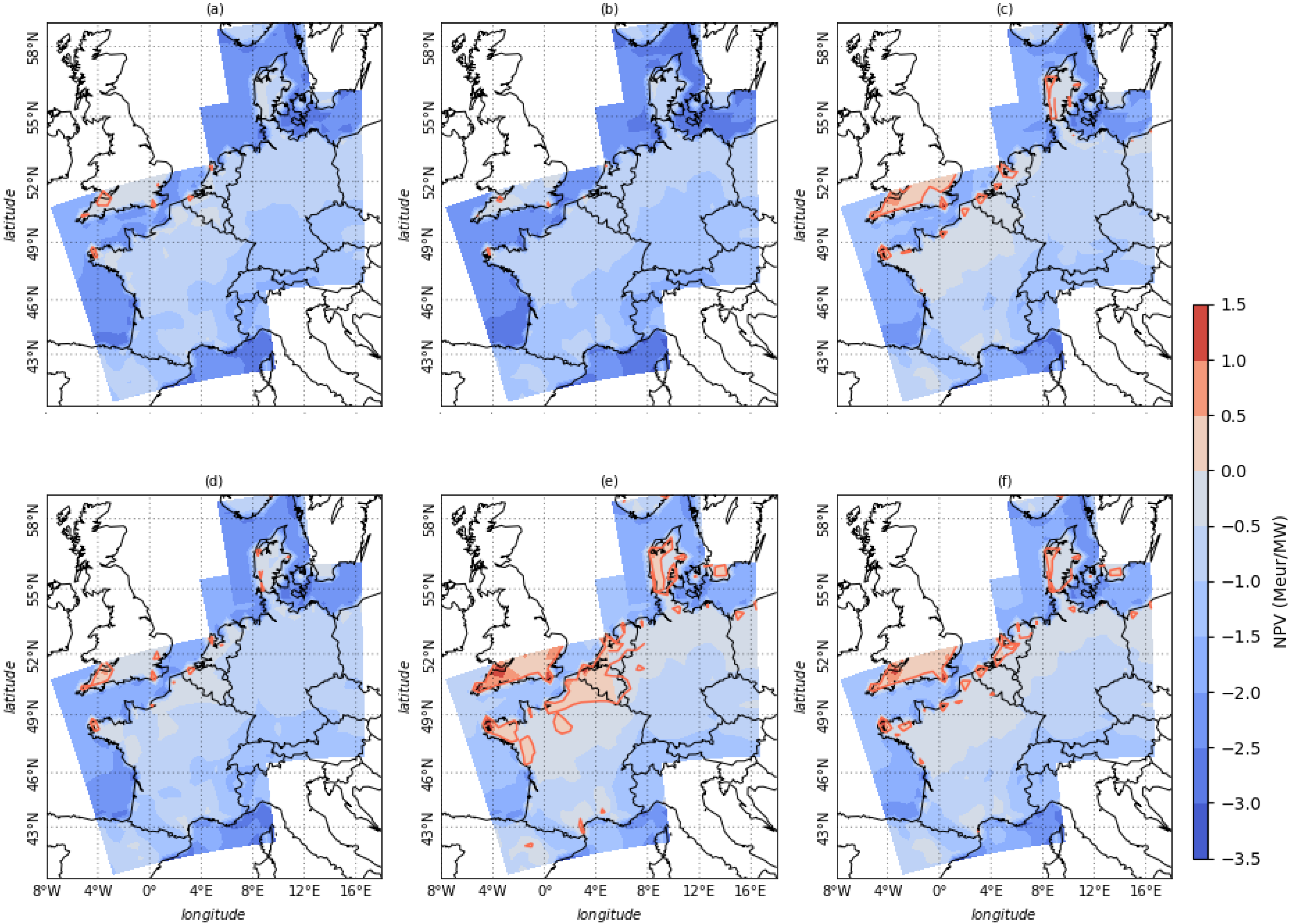
From our synthetic dataset of 111 years, we define 81 virtual wind farm projects at each gridpoint starting on the 1st of January of each year from year 1 to year 82 and lasting 30 years. Figure 7 displays the NPV averaged over 81 project at each gridpoint, as well as the corresponding (quantile at the 95% level).
For offshore wind farms operating without subsidies (Figure 7a,b), the NPV is negative due to the high initial investment and costs. Thus, offshore wind farms are not yet profitable if not supported by regulations mechanisms. Nevertheless, both investment costs and operational costs are rapidly decreasing [5,20,38]. For onshore wind farms, small areas in the west of France display small positive NPV of the order of the range between the mean and the 95th percentile of NPV. The difference between the mean and the is small, meaning that the NPV does not vary much on the long term. The standard deviation is less than 5% the mean of the NPV in most of the regions.
Note that removing the trends in the ERA20C wind speed to compute local production has a large impact on the inter-quartile range (IQR) for the 81 projects: using detrended production results in an IQR which is 30% to 100% lower than the IQR computed using production with trends. In other words, the very long-term trends in wind speed result in low profitability early in the century and higher profitability at the end of it. Detrending wind speed results in a less varying profitability along the 20th century. The decrease in IQR is larger for offshore wind farms and for onshore wind farms close to coast.
We model both the feed-in-tariff (henceforth FiT) and the feed-in-premium (henceforth FiP) subsidy. Under FiT, the producer receives a fixed guaranteed price of 82 €/MWh for 10 years after which the price decreases linearly for 5 years to 28 €/MWh. After 15 years the subsidy disappears and the remaining energy is sold in the day-ahead market. This corresponds to the support mechanism used in France until 2016. The function , which defines the amount a producer receives for a MWh produced, is given by:
Several FiP procedures exist. We choose to use a simplified one under which the producer receives a guaranteed bonus of 33 €/MWh in addition to the market price. After 15 years, the subsidy disappears and the remaining energy is sold in the day-ahead market. The function is, in this case, given by:
The formula for the bonus is inspired from the Danish FIP. In reality, the procedure is slightly different, as the bonus is guaranteed until the sum of the the price and the bonus is under . In this last case, the producer receives a bonus to reach the target of . Germany used a FiT mechanism similar to the French one until 2012 and now uses a FiP similar to the Danish one. We use the same mechanisms for onshore and offshore wind farms.
For wind farms supported by either FiT (Figure 7c,d) or FiP (Figure 7e,f) mechanisms, the wind farm value is higher, especially in the case of the FiT mechanism. Offshore wind farms are found to be profitable with FiT in the Western coast of France, Denmark, and Germany. The average NPV over the 81 projects for the FIT mechanism reaches 2.5M €/MW for a wind farm with a lifetime of 30 years (Figure 7c). For FiP mechanism, the average NPV reaches 2.3M €/MW (Figure 7e). The difference between the mean and the is still small and represents not more than 10% of the mean NPV, showing that the revenues are rather stable in this case. A sensitivity analysis of NPV with respect to the discount rate is reported in the Appendix (Methods section).
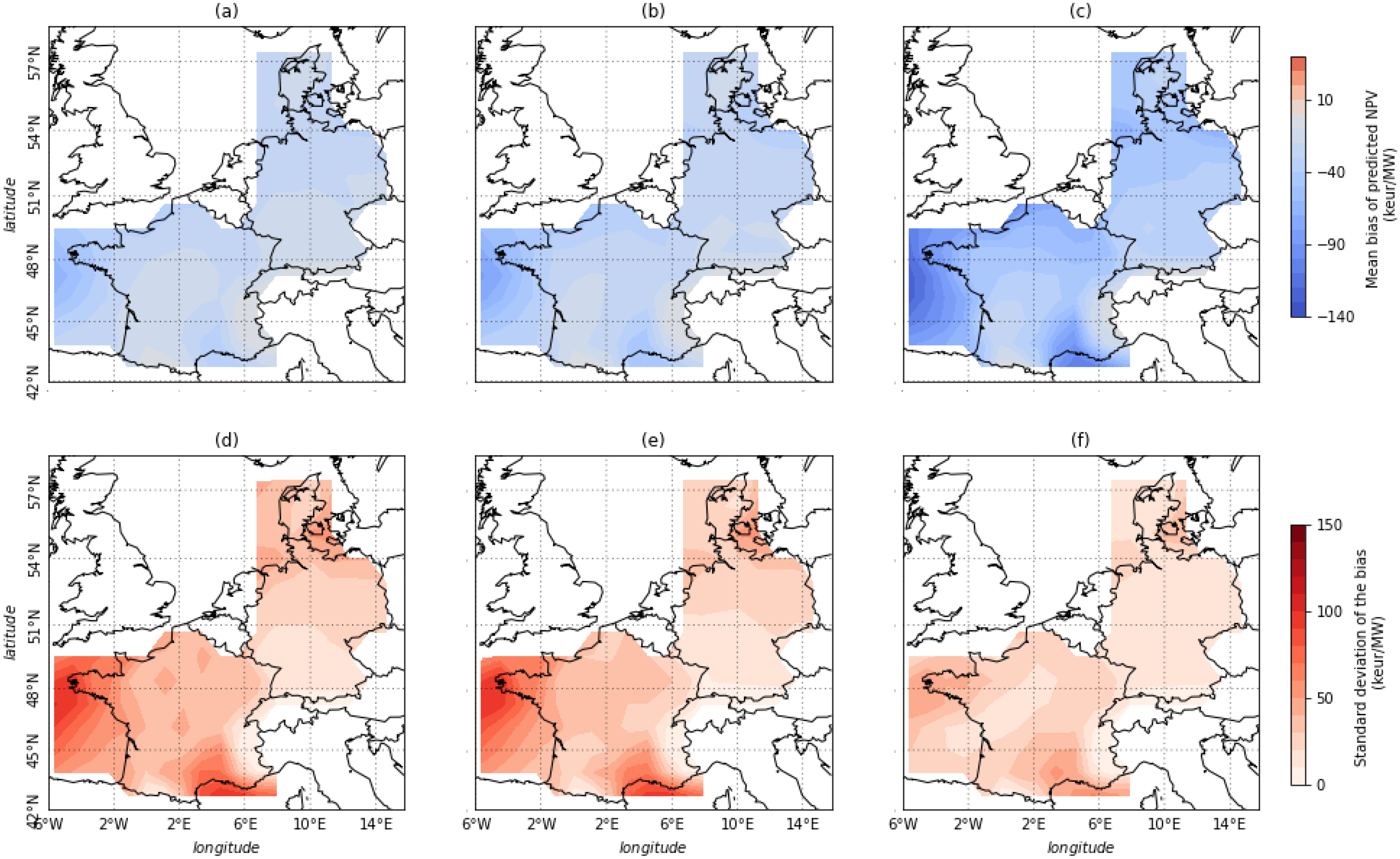
It is common for a wind farm project to base the projections for the future value of an asset on the historical wind speed recorded at the chosen location. To highlight the shortcomings of this approach, we define 51 wind farm projects at each gridpoint starting on the first of January of each year from year 31 to year 82 and lasting 30 years The choice of 51 projects is due to the fact that we have 111 years of data and would like to have 30 years of observations before the start of the project in order to test different projection strategies. We use three different strategies for estimating the wind farm value: the first one based on the wind speed recorded during 5 most recent years, the second one based on 10 most recent years, and the third one based on 30 most recent years before the project begins. Figure 8 displays the mean bias and standard deviation of the bias between projected NPV and actual NPV. We compare projections based on a historical period of 5 years (Figure 8a,d), 10 years (Figure 8b,e), and 30 years (Figure 8c,f).
Our results show that every method underestimates the average NPV. Using the past 30 years to project future revenues results in a larger mean error (underestimation) than using 5 or 10 past years (Figure 8a compared to Figure 8b,c). Nevertheless, the standard deviation is much lower using this method (Figure 8f than using the 5 or 10 past years of data (Figure 8d,e). Thus, using 5 or 10 past years results in higher risk to make large errors than when the projection is based on a longer period (e.g., 30 years). Using 30 years of data makes the projection more sensitive to very long term trends, resulting in a larger mean error, while using fewer historical years makes the projection more sensitive to shorter term interannual variability of revenues. Such projections can sometimes largely overestimate or underestimate the actual future production, revenues and wind farm value. For instance, if an investor projects future revenues based on the past 5 years when the NAO is in positive phase, he may highly overestimate future production concluding wrongly on the profitability of the project.
Note that this result is very sensitive to long term trends found in ERA-20C wind speed. Indeed, the fact that the mean error is larger for a projection based on 30 years than a projection based on 5 years is entirely due to these trends. When trends are removed from the data, using the past 30 years to project future revenues results in a lower mean bias than when using 5 or 10 past years, so that this method becomes the best in terms of both mean and standard deviation of the error.
4. Future Value of Wind Farms under Realistic Socio-Economic Scenarios and Climate Change
In this illustration we compute the NPV for virtual wind farms commissioned on 1st January 2021 with a lifetime of 30 years (decommissioning date is 31st December 2050). Figure 9 displays the NPV averaged over the 10 CORDEX simulations (5 models and 2 RCPs), for each of the 6 price scenarios, in the case of wind farms operating without support mechanism. In the scenario of high electrification and low penetration of wind energy (Figure 9d), several areas of the domain are found to be profitable for onshore wind farms. In the northwest of France and in the western coast of Denmark, the NPV attains 1 M €/MW without support mechanisms. In the remaining scenarios, positive NPV is very rare and in any case very low. As a consequence, in most cases, support mechanisms are needed to guarantee profitability of wind farms and thus ensure energy transition.
Level and Cost of Support Mechanisms under Future Climate
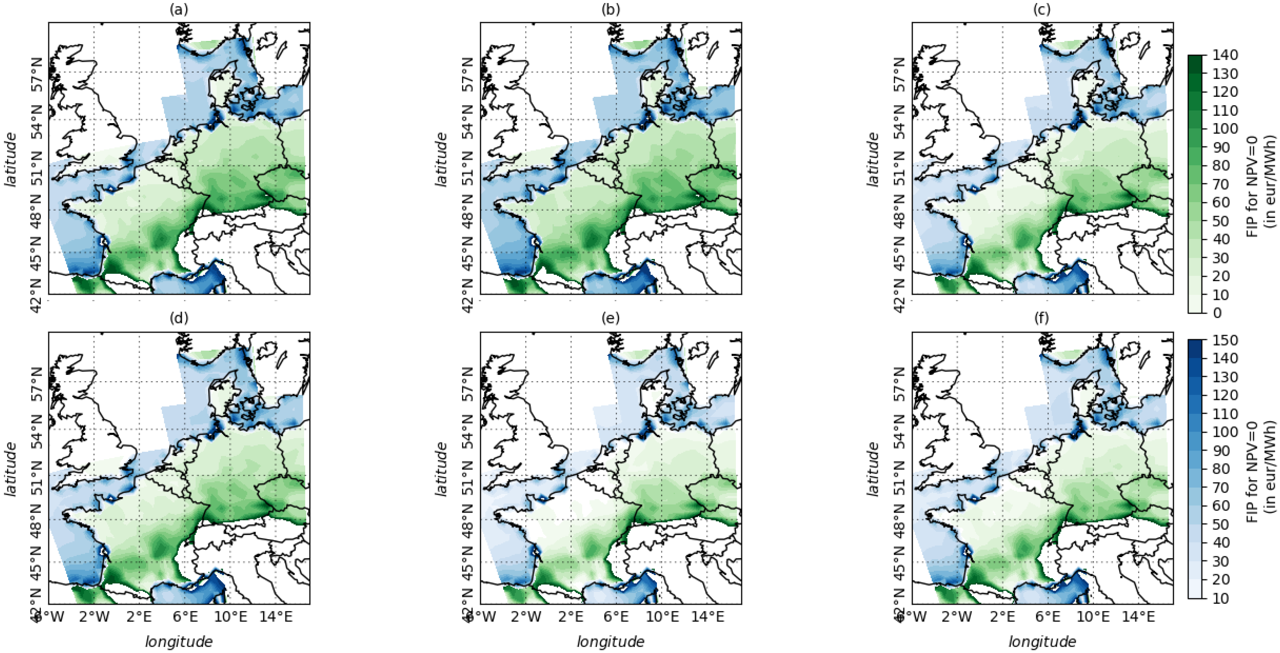
Figure 10 maps the FiP level needed to guarantee a positive or null NPV for wind farms installed in 2021 and operating for 30 years under each considered scenario. The FiP is a simple premium added to the market price for the first 15 years of plant’s operation: the FiP takes into account the evolution of the market price, contrary to the FiT which is less dependent on prices (the dependence only appears at the mechanisms’ expiration date, i.e., after 15 years).
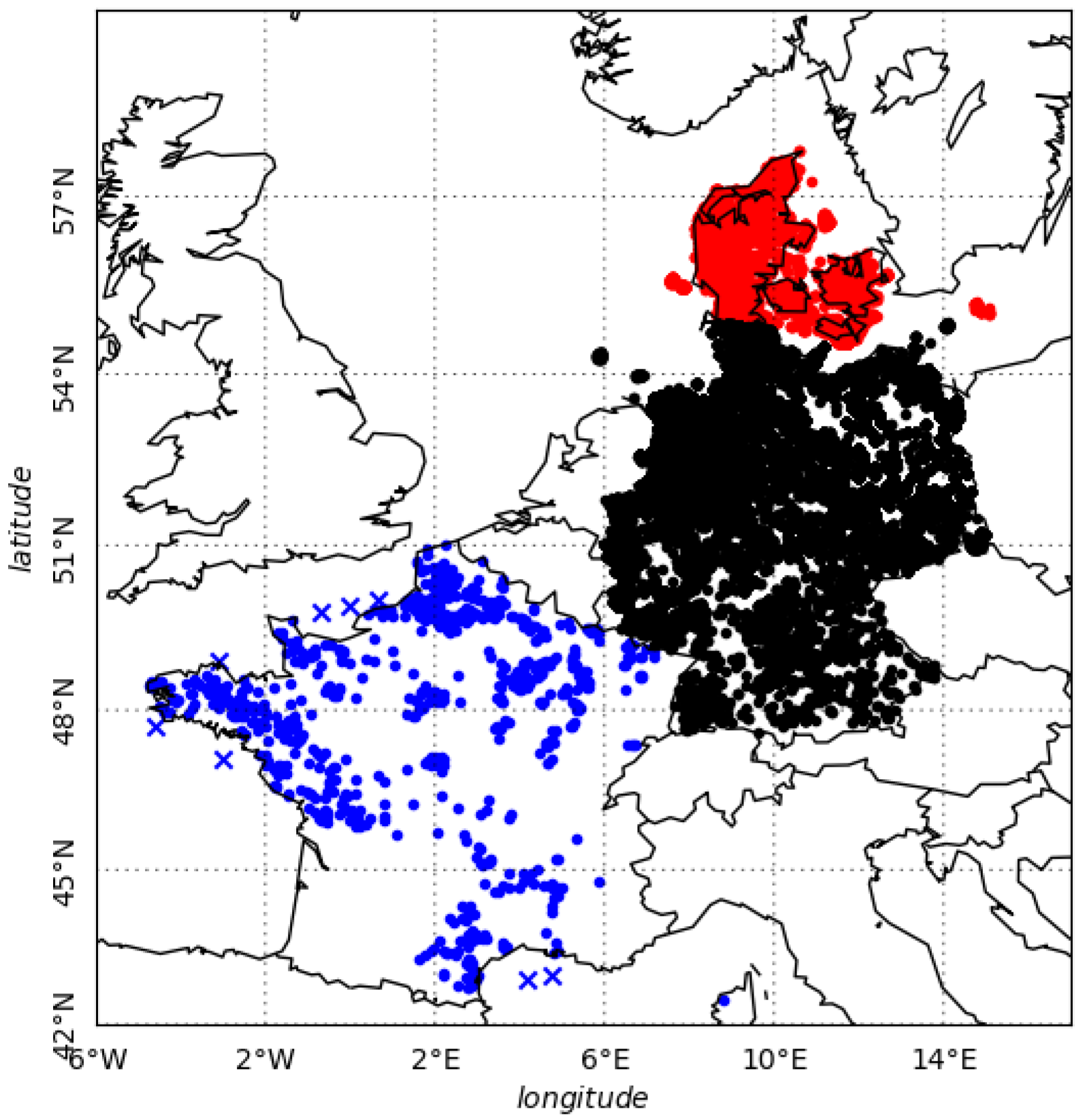
Using the current spatial distribution of the wind farms in the three countries under study (Figure 11), we calculate for each country the premium level needed to guarantee a positive NPV for the 90% of the fleet. We assume that the new installed capacity will display the same spatial distribution as the current one. For offshore wind farms in France, where there is no currently installed capacity, we make the assumption that future wind farms will be mainly placed in the northern coast and in the south, close to the shore (see Figure 11).
In France, the premium level for onshore (offshore) wind farms varies from 33 €/MWh (45 €/MWh) in the best case scenario (Figure 10e) to 66 €/MWh (78 €/MWh) in the worst case scenario (Figure 10b). In Germany, the premium level for onshore (offshore) wind farms varies from 68 €/MWh (76 €/MWh) in the best case scenario (Figure 10e) to 93 €/MWh (102 €/MWh) in the worst case scenario (Figure 10b). Finally, in Denmark, the bonus level for onshore (offshore) wind farms varies from 1.5 €/MWh (83 €/MWh) in the best case scenario (Figure 10e) to 23 €/MWh (105 €/MWh) in the worst case scenario (Figure 10b).
With these data, we are able to calculate the cost of wind energy penetration (onshore and offshore) for each country and in each scenario. Remember that, for scenarios 2, 4, and 6, penetration is high, i.e., total (new) installed capacity in France in 2030 is 41 GW onshore and 11.1 GW offshore; in Germany 71 GW onshore and 20 GW offshore; and in Denmark 6.5 GW onshore and 6.1 GW offshore. In scenarios 1, 3, and 5, penetration is low, i.e., total (new) installed capacity in France is 31 GW onshore and 4.3 GW offshore; in Germany 60 GW onshore and 14 GW offshore; and in Denmark 3.6 GW onshore and 3.4 GW offshore. Note that we not only consider the cost of new installed wind farms, but also that of the replacement of current installed wind farms. Indeed, the vast majority of the currently installed wind farms will arrive at decomissioning date within the next 30 years so that they will need to be replaced to reach the penetration given by our scenarios. The costs are computed by simply adding up the future payments, without discounting, and, as a result, we may slightly overestimate the true costs. However, these are public support policy costs which should therefore be discounted with the sovereign borrowing rate, and the sovereign bond rates are presently quite low.
We find that supporting the penetration of wind energy (over the 15 years of support) will cost the regulator from EUR 57 to 172 billion in France, from EUR 232 to 397 billion in Germany, and from EUR 18 to 50 billion in Denmark, depending on the scenario considered and the level of penetration of wind energy. The results for each scenario are shown in Figure 12. Scenario 5 always results in lower cost for the regulator due to higher electricity prices and low penetration. Conversely, Scenario 2 results in higher costs for the regulator because of the price decreases coupled with high penetration.
5. Discussion and Policy Implications
The first objective of our paper was to evaluate the net present value of standardized wind farms and quantify the associated uncertainty. Our results show that the extreme variations of net present value along the 20th century are of the order of one year of revenues whatever the support mechanism used. We show that under recent climate and current market prices, profitability of wind farms is not guaranteed without support schemes. Using feed-in tariff (FiT) and feed-in premium (FiP) mechanisms with current level of support allows to guarantee profitability of wind farms in a large part of the domain. We also show that when projecting the future value of a wind farm based on historical production records, an investor can both overestimate or underestimate the profitability due to the natural variability of wind speed and to the presence of long-term trends.
Our second objective was to quantify the support level that will be needed in future to guarantee the profitability of the wind fleet, and to evaluate the cost of such support mechanisms. To address this objective, we simulated future price scenarios using electricity demand and renewable penetration projections from integrated assessment models. These scenarios were combined with wind speed and temperature projections from the regional climate model intercomparison project (CORDEX), corresponding to several Representative Concentration Pathways (RCP). This enabled us to model future local wind energy production and prices in a changing climate. Our approach allows to assess and quantify several relevant sources of uncertainty [39]: socio-economic uncertainties corresponding to the choices made by the society (e.g., the extent of climate change mitigation vs. adaptation), scientific uncertainties (corresponding to model simulations spread and associated with modelling errors), and natural/climate uncertainties (related to the natural variability of the earth system, including climate change).
Under future climate scenarios, we show that profitability of wind farms is reached in several regions of the domain only in the specific scenario of high electrification and low penetration of wind energy. To guarantee profitability of 90% of the wind farms in the future, under the assumption that future wind fleet is installed following current spatial distribution, the required premium level in France for onshore (offshore) wind farms varies from 33 €/MWh (45 €/MWh) in the best case scenario to 66 €/MWh (78 €/MWh) in the worst case scenario. In Germany, the premium level for onshore (offshore) wind farms varies from 68 €/MWh (76 €/MWh) in the best case scenario to 93 €/MWh (102 €/MWh) in the worst case scenario. In Denmark, the premium level for onshore (onshore) wind farms varies from 1.5 €/MWh (83 €/MWh) in the best case scenario to 23 €/MWh (105 €/MWh) in the worst case scenario. According to these results, we find that supporting the penetration of wind energy in these countries during 15 years amounts to costs for the regulator ranging from EUR 3.8 to EUR 11.5 billion per year in France, from EUR 15.5 to EUR 26.5 billion per year in Germany, and from EUR 1.2 to EUR 3.3 billion per year in Denmark, depending on the scenario considered and the level of penetration of wind energy. In the preceding section, we computed aggregate costs for the period of 15 years, and here they are reported on a yearly basis to make comparisons easier.
These numbers should not be interpreted as global investment needs, but rather as costs of public support measures required to attract the necessary investments from the private sector. Let us compare them with the current support measures for wind energy in the three countries we analyse in this paper. In France, where the renewable energy penetration is the lowest among the three countries, the cost of public support measures for the wind energy industry amounted to EUR 1.2 billion in 2018, in Germany this number was EUR 9.7 billion, and in Denmark EUR 0.45 billion [40]. However, one needs to keep in mind that between 2012 and 2018, the renewable energy subsidies in the EU grew by about 4% per year, and given the current plans for massive deployment of renewables, further growth should be expected. The fact that our estimates for the future support needs are higher than the current subsidies can be explained, firstly, by the need to accelerate the energy transition to be able to meet the Paris Agreement goals, secondly, by the fact that at present when the number of wind farms is relatively low (especially in France), they are installed at the most profitable locations, which may no longer be available in future, and thirdly, by our modeling assumptions, some of which may introduce an upward bias. Let us briefly recall these assumptions here.
- Our analysis is based on the assumption (which is the actual situation in many countries) that the subsidy mechanism (feed-in tariff or feed-in premium) is the same for all wind farms within a country, and is not adjusted depending on the profitability of each specific farm. We have chosen, somewhat arbitrarily, to fix the parameters of the mechanism so that 90% of the farms are profitable. Our methodology can, of course, be used with any other number. This means that 10% of the farms do not receive a sufficient subsidy, and for 90% of the farms, the subsidy is higher than the minimum amount to ensure profitability. If the subsidy were determined individually for each site, as in renewable energy auctions, which are increasingly more common, each farm would receive just the required subsidy amount and the overall cost would be lower.
- Our analysis is completed assuming current market conditions, and, therefore, does not take into account the possible increase in carbon taxes/carbon costs, which are a key tool for energy transition and GHG emission reduction. By making electricity production with fossil fuels more expensive, carbon taxes make renewable producers more competitive. The revenues of renewable producers increase and this can be seen as an indirect subsidy, albeit at a cost to electricity consumers in the form of higher prices. For the same technology, this cost will generally be higher than the cost of direct subsidies, since higher electricity price is paid to all producers, whereas targeted subsidies are only paid to renewable producers. However, this can be partly compensated by distributing a part of the carbon tax to more vulnerable consumers, to also address the social issues of the energy transition. In our paper, the carbon prices are not taken into account directly, although the electricity demand scenarios from integrated assessment models we use may account for carbon pricing. We do not model carbon taxes directly since imposing carbon taxes is largely a political decision and their modeling requires assumptions on environmental policies of the concerned states, which may turn out to be incorrect. However, our results can be seen as an estimate of the cost of future renewable production, to be paid to renewable producers either in the form of subsidies or in the form of higher prices.
- Finally, our estimates do not take into account the potential reduction in costs of wind energy. Indeed, renewable energy production costs are declining. This decline is more significant for solar energy than for wind energy. For example, in a recent article [3], the capital expenditure for solar power plants is predicted to drop by 75%, while a drop of 40% is expected for onshore wind turbines. Since in our study new wind turbines are installed every year from 2020 to 2035, we can expect an average reduction of 10% in the CAPEX, which would lead to a reduction in the cost of public support measures of at least a similar magnitude.
Policy Implications
As the wind and solar energy industries mature, there is a tendency to phase out the subsidies for wind and solar energy production, and some new plants at particularly profitable locations are already being built without public support, see https://qz.com/1995355/the-era-of-subsidies-for-wind-and-solar-is-coming-to-a-close/ (last accessed on 8 August 2022). This is especially true for the solar energy, where, on the one hand, the capital costs are decreasing fast, and on the other hand, the cost of subsidies is higher in most countries [41], and their impact per euro spent in terms of GHG emission reductions is lower than for the wind energy [21]. However, our analysis shows that accelerating the deployment of wind energy at the rate required for a successful energy transition may require maintaining and even increasing the level of public support. This is consistent with the estimates of IRENA which projects a 26% increase in renewable energy subsidies between 2017 and 2050 [42]. Our second message is that while with the historical support measures, such as feed-in tariff and feed-in premium the required subsidies may be high, the variability of renewable energy output is such that using site-specific measures, such as renewable energy auctions may considerably reduce the need for public support.
6. Conclusions
In this study, we quantify the net present value of standardised wind power plants and the associated uncertainty in France, Germany, and Denmark under present and future climate, and we evaluate the cost of the support schemes needed to ensure the economic sustainability of the wind energy industry. The main contribution of our research is to combine, on the one hand, the information on the wind resource from reanalysis and climate scenarios, and on the other hand, information on energy prices from a model of electricity consumption based on climate data and economic scenarios. Building a realistic model for future wind farm revenues is a complex task and some important features had to be left to further research. First, the evolution of capital and operational costs of wind energy is not taken into account. The model for electricity prices does not include socio-economic factors other than electricity consumption and renewable energy production, such as, for example, fuel costs, or geopolitical uncertainty, which can temporarily lead to very high electricity prices as in 2021–2022. The economics of a wind farm is stylised, both in terms of revenues (we assume that it is given by the market price plus a premium but, for example, the role of aggregators is not taken into account) and in terms of wind production (we use the same turbine model everywhere with only a correction factor for offshore turbines). The price and consumption models are fitted over a relatively short 3-year period, and, for example, the bias in the reanalysis data is assumed to be constant in time.
Despite these limitations, our work provides an original integrated methodology to assess the uncertainties of wind farm net present value under current and future climate. The methodology is fairly general and it can be easily applied to other countries. The results of our analysis highlight the fundamental role that support schemes play and are likely to be playing in the future in guaranteeing the economic viability of wind power plants. Our study provides an estimate of the future costs of wind energy deployment, and a quantification of its uncertainty under different climate and socio-economic scenarios. We show that the final cost to achieve energy transition by supporting wind penetration is not negligible and that it can vary widely across countries.
In the future development of our methodology, the first step will be to include a more realistic model for electricity price formation, taking into account the merit order stack of electricity markets, the carbon price, and the stochastic evolution of fuel prices. The evolution of capital costs of wind power plants, with a realistic learning curve, will be an important building block. Finally, the social aspects of energy transition, from public acceptance of wind power plants to obstacles posed by rising energy prices will be taken into account.
Author Contributions
Conceptualization: B.A., S.C., A.C., P.D. and P.T.; methodology: B.A., S.C., A.C., P.D. and P.T.; software: B.A.; data curation: B.A.; writing—original draft preparation: B.A. and P.T.; writing—review and editing: B.A., S.C., A.C., P.D. and P.T.; visualization: B.A.; supervision: S.C., A.C., P.D. and P.T.; project administration: P.T.; funding acquisition, P.D. and P.T. All authors have read and agreed to the published version of the manuscript.
Funding
This work was carried out at the Energy4Climate Interdisciplinary Center (E4C) of IP Paris and Ecole des Ponts ParisTech, supported by 3rd Programme d’Investissements d’Avenir [ANR-18-EUR-0006-02]. It was funded by the Tuck Foundation (grant FoE-FA-2018-3-01) and Labex ECODEC (ANR-11-IDEX-0003/LabexEcodec/ANR-11-LABX-0047). The work of Anna Creti and Peter Tankov is additionally supported by the ANR Project EcoREES (Economic Sustainability of the Future Highly Renewable European Energy System, grant ANR-19-CE05-0042) and the work of Peter Tankov by the project SECRAET (Scenario-Based Climate Risk Analysis for Energy Transition) funded by ADEME and by the FIME Research Initiative. Silvia Concettini acknowledges the support of the Chair Energy and Prosperity, under the aegis of the Fondation du Risque.
Institutional Review Board Statement
Not applicable.
Informed Consent Statement
Not applicable.
Data Availability Statement
The datasets produced within this project is available on request from E4C Datahub at https://www.e4c.ip-paris.fr/#/fr/datahub/projects (last accessed on 8 August 2022).
Conflicts of Interest
The authors declare no conflict of interest.
Abbreviations
The following abbreviations are used in this manuscript:
| CAPEX | capital expenditures |
| CMIP5 | coupled model inter comparison project version 5 |
| CORDEX | coordinated regional downscaling experiment |
| ENTSOE | European network of transmission system operators for electricity |
| FiP | feed-in premium |
| FiT | feed-in tariff |
| IAM | integrated assessment model |
| IQR | interquartile range |
| MSLP | mean sea-level pressure |
| NAO | North-Atlantic oscillation |
| NPV | net present value |
| OPEX | operational expenditure |
| RCM | regional climate model |
| RCP | representative concentration pathway |
| RSD | relative standard deviation |
| RTE | réseau de transport de l’électricité |
| VaR | value at risk |
Appendix A. Methods
Appendix A.1. Data
The data employed in this study have either an economic or a meteorological nature. A summary of the variables and the data sources is provided in the Table A1. Economic data consist of historical electricity consumption, production and price data at the national level; meteorological data are surface temperature and wind speed which are retrieved from reanalysis and regional climate models (RCM) at the local scale (model gridpoints).

Table A1.
Datasets.
| Source | Variable | Name | Period | Time Resolution |
|---|---|---|---|---|
| ENTSOE | Electricity demand | 1 January 2015 to 31 December 2018 | hourly | |
| Wind production | 1 January 2015 to 31 December 2018 | hourly | ||
| Day-ahead prices | 1 January 2015 to 31 December 2018 | hourly | ||
| RTE | Regional capacity factor | 1 January 1979 to 31 December 2017 | monthly | |
| ERA-5 | Surface temperature | 1 January 1979 to 31 December 2018 | hourly | |
| Surface wind speed | 1 January 1979 to 31 December 2018 | hourly | ||
| ERA-20C | Surface temperature | 1 January 1900 to 31 December 2010 | 6-hourly | |
| Surface wind speed | 1 January 1900 to 31 December 2010 | 6-hourly | ||
| CORDEX (see Table A2) | Surface Temperature | 1 January 1971 to 31 December 2005 and 1 January 2006 to 31 December 2100 | daily | |
| Surface wind speed | 1 January 1971 to 31 December 2005 and 1 January 2006 to 31 December 2100 | daily |
We obtain the hourly demand (), production (), and day-ahead price () for France, Germany, and Denmark between 1 January 2015 and 31 December 2018 from the European Network of Transmission System Operators for Electricity (ENTSOE) website.
RTE (Réseau de Transport d’Électricité) website provides the observed regional monthly wind capacity factors in the French regions between January 2015 and December 2017.
As a proxy for past climate, from ERA-5 reanalysis ([43]) and ERA-20C reanalysis ([44]), we retrieve surface temperature () and surface wind speed () over the domain covering France, Germany, and Denmark (Figure A1).
The ERA-20C reanalysis spans the period from 1 January 1900 to 31 December 2010, at 6-hourly time resolution and spatial resolution. The ERA-5 reanalysis spans the period from 1 January 1979 to 31 December 2018, at hourly resolution and spatial resolution. The spatial resolution of ERA-20C is very coarse (>100 km in longitude and latitude). As a consequence, the results presented in the study give a broad cartography of wind farms profitability and do not take into account small scale phenomena, such as small scale topography effect on wind (forests, hills, buildings…). The ERA-5 data are much more resolved spatially (<20 km in longitude and latitude). It also assimilates observations from satellites which where launched in the late 1970s. Moreover, this reanalysis is more recent than the ERA-20C reanalysis, so that it is considered more reliable. Last, but not least, the time period covered by ERA-5 reanalysis overlaps with the wind production, electricity demand, and electricity price observations used in this study. Unfortunately, the ERA-5 reanalysis spans a relatively short time period which does not allow to carry out a deep investigation of the variability within the entire 20th century. Therefore, we the ERA-5 dataset to calibrate models and to correct the bias of the longer ERA-20C dataset, but then use the ERA-20C data to construct the long time series of electricity price and wind power production.
Figure A1.
Domains and onshore and offshore masks in ERA20C data. Note: onshore (figures (a–c)) and offshore (figures (d–f)) masks are drawn for each country to highlight the difference between onshore wind farms which have a lower capacity factor and lower costs and offshore wind farms.
Figure A1.
Domains and onshore and offshore masks in ERA20C data. Note: onshore (figures (a–c)) and offshore (figures (d–f)) masks are drawn for each country to highlight the difference between onshore wind farms which have a lower capacity factor and lower costs and offshore wind farms.

For future climate projections, we use simulations from the Coordinated Regional Downscaling Experiment (CORDEX) program ([45]) which aims at developing an improved framework for generating regional-scale climate projections. We retrieve daily surface temperature and daily surface wind speed from historical RCP-4.5 and RCP-8.5 simulations of several Regional Climate Models (RCMs) listed in the Table A2 over the European domain (EUR44) with spatial resolution of . The historical simulations span from 1 January 1971 until 31 December 2005, and the RCP-4.5 and RCP-8.5 simulations span the period from 1 January 2006 until 31 December 2100. In this paper, we limit the period of study to 31 December 2050.
Table A2.
List of the CORDEX model simulations used in the study.
| Institution | Model Used |
|---|---|
| IPSL-INERIS | IPSL-CM5A-MR |
| DMI | ICHEC-EC-EARTH |
| CLM-Com | MPI-M-MPI-ESM-LR |
| MPI-CSC | MPI-M-MPI-ESM-LR |
| SMHI | NOAA-GFDL-ESM2M |
Appendix A.2. Models
Appendix A.2.1. Demand Model (Model Dn)
The daily electricity demand is modelled as a function f of the mean daily surface temperature in France at time t, and of threshold temperatures with h for “hot” and with c for “cold”:
Here, and are parameters, which are found by non-linear least squares, W is the set of weekdays, O is the set of weekend days/holidays, and is a residual.
The functional forms are specified as follows,
Appendix A.2.2. National Production Model (Model Wn)
The daily wind energy production is computed from observed data from ENTSOE. The daily wind speed at 10 m is first extrapolated to 100 m (hub height) using the power law with [46]:
Next, the power curve of Figure A2 is applied at each gridpoint with . We compute the mean wind energy production onshore and offshore as:
with the power computed at each gridpoint and the installed capacity in the given country at time t. A bias still exists between computed and observed production because the installed capacity is observed at the country scale. In order to correct this bias, we apply, separately for onshore and offshore production, a linear least square regression to obtain . Adapting the a parameter to obtain more realistic capacity factors (Figure A2) for each offshore and onshore location would lead to comparable results. However, we prefer to correct the bias using the observed national production data from ENTSOE.
Figure A2.
Power curve of a Vestas-90-2MW Turbine with normalized power.

Appendix A.2.3. Day-Ahead Price Model (Model P)
Let us denote the hourly price as and the daily price as , and let . We denote weekdays and weekend days/holidays with superscripts and , respectively, as for the demand model, and the superscript means that the expression holds both for weekdays and for weekends.
We first decompose and using Principal Component Analysis as:
Here, is the mean daily cycle around , is the mode of variation of the daily cycle and is the so called principal component that shows how the given mode of variation evolves with time.
In our price model, we fix the number of principal components to and model the dynamics of and . Introduce the vectors
The dynamics of each vector is described by an autoregressive model involving the demand , the national wind production , seasonal and autoregressive components.
The parameters , , , , , are fitted by least square regression. We assume that the residuals follow a hyperbolic distribution, whose parameters are estimated by maximum likelihood.
The full model for the price process can then be written:
where, as before, W denotes the set of weekdays and O is the set of weekend days/holidays.
Appendix A.2.4. Local Wind Speed and Production Models (Model F and W)
The model F aims at generating an hourly wind speed time series from the 6-hourly (resp. daily) wind speed from ERA-20C reanalysis (Cordex simulations) that is statistically consistent with hourly wind speed from ERA-5 reanalysis.
Assume that the logarithm of the wind time series, , is an Ornstein–Uhlenbeck process with dynamics:
The explicit form of the OU process is
The stationary law of this process is
and the autocorrelation in the stationary regime is . The model parameters , k, and can thus be easily estimated from the mean, variance, and autocorrelation of the log-wind time series.
We would like to characterise the law of given for . It is clear that the conditional law of given is Gaussian. We thus only need to characterise the mean and the variance .
Let
Then, is independent from . Therefore,
and
With these known values of mean and variance, on can easily simulate the value of . This enables us to simulate the 10 m wind speed at the hourly time resolution, which we denote in the following by , by interpolating the 6-hour time series.
The model W aims at modelling the local wind energy production from . We first extrapolate wind speed to height using power law [46]:
with .
Finally, we apply the power curve of a Vestas-90 (2MW) wind turbine (Figure A2) with normalized power to obtain the local wind capacity factor. In order to take into account differences between onshore and offshore wind turbines, we define and to be equal to and , respectively. The values of and have been chosen to obtain an average capacity factor onshore and offshore of and , respectively.
Appendix A.3. Validation
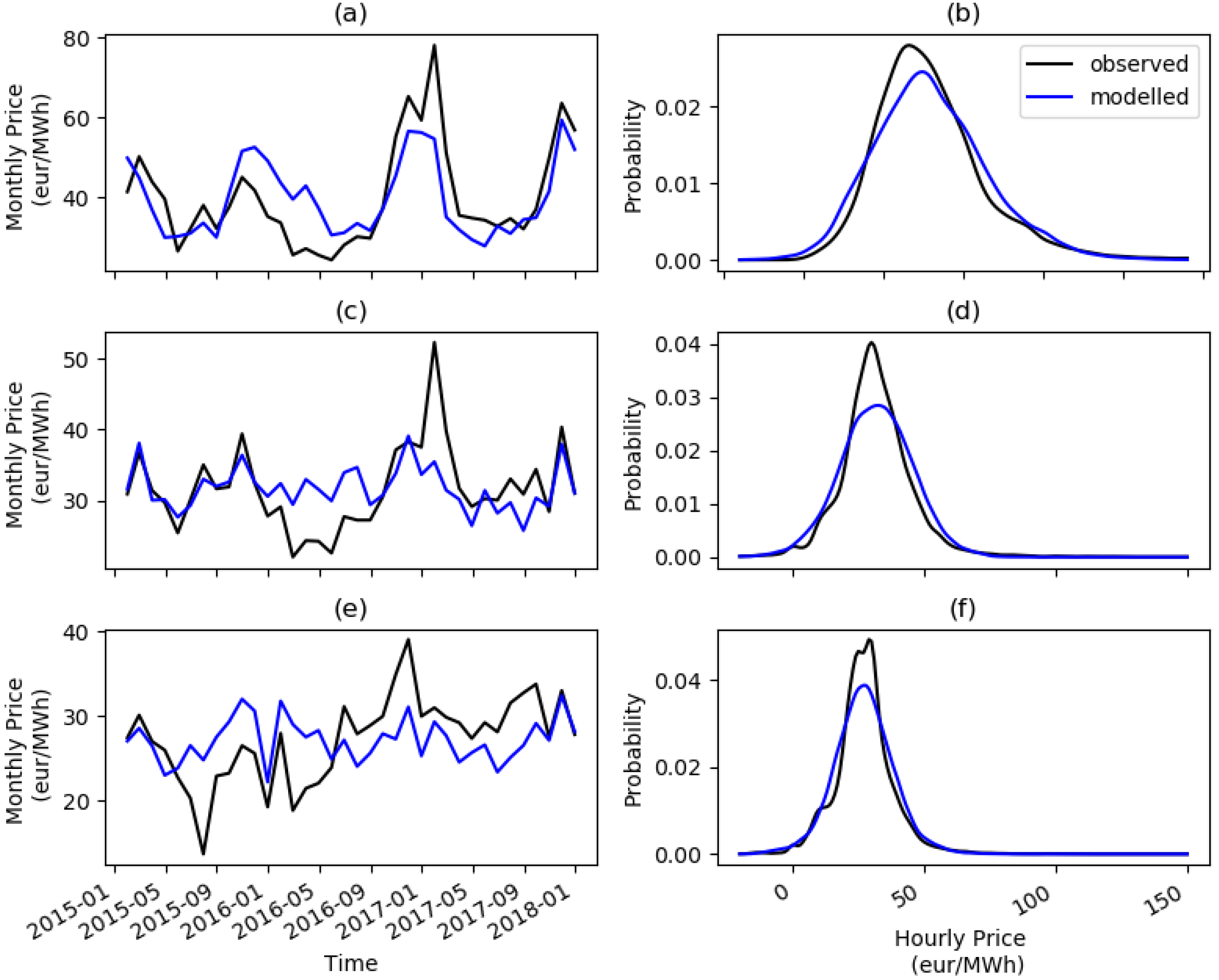
Left panels in Figure A3 display the time series of monthly average prices between 1 January 2015 and 31 December 2017, distinguishing between observed values from ENTSOE (in black) and modelled ones (in blue). Values for France, Germany and Denmark are shown in panel (a), (b), and (c), respectively. Right panels present the distributions of hourly prices for the same period in France (b), Germany (d), and Denmark (f).
Figure A3.
Time series (left) of monthly average prices and estimated probability density function of hourly prices for the period between 1st January 2015 and 31st December 2017. France: (a,b); Germany: (c,d); and Denmark: (e,f).
Figure A3.
Time series (left) of monthly average prices and estimated probability density function of hourly prices for the period between 1st January 2015 and 31st December 2017. France: (a,b); Germany: (c,d); and Denmark: (e,f).

Time series of monthly average prices show a satisfying correlation (0.74) in France due to a well modelled seasonal cycle (Figure A3a). Several peaks and lows are well reproduced by the model (in December 2017 for instance). In Germany, the correlation (0.56) is also satisfying, even if the seasonal cycle seems to be underestimated (Figure A3c). The peaks during 2016/2017 winter are not precisely reproduced in France and Germany because they are related to a particular situation in Western Europe when nuclear plants in France had very low availability and the hydro-reservoirs had low levels. Our model is unable to reproduce such peaks because availability of nuclear and hydro is not taken into account. This kind of special situations are rare and we leave them out of the scope of the paper.
For what concerns hourly prices in France and Germany (Figure A3b,d, respectively), we find that the modelled prices have a slightly higher variance compared to the observed prices. This indicates that price volatility is slightly overestimated in our model. This may be due to spikes in observed time series which induce small errors in hyperbolic law parameters estimation (see the Methods section) and which we choose not to model for simplicity.
In Denmark, the model seems to be less efficient as the correlation between observed and modelled monthly average prices is lower (0.31, significant at 0.05 confidence level) (Figure A3e). Indeed, in Denmark, electricity prices are much more volatile and more subject to spikes than in France and Germany, which makes them harder to model. Still, the distributions of observed and modelled hourly prices are close to each other (Figure A3f), with the same kind of volatility issue as in France and Germany.
To validate the local production model, we use regional monthly capacity factors from RTE website. On the basis of the results found for France, we can validate the model for the other countries. Indeed, France displays a large panel of regions which have their own particularity (e.g., land and sea area; flat terrain and mountainous regions; large scale pressure system induced winds in the northwest and regional winds induced by air channeling in the southeast). In Denmark and Germany, the terrain is mainly flat, and wind speed is mainly driven by large scale pressure system. Thus, the wind speed in Denmark and northwestern Germany varies such as northwestern winds in France. The method for modelling production from reanalysed wind speed being the same in all countries, there is no reason for Danish and German production to display larger deviation from monthly capacity factor than in France. Therefore, the production in the northwest of France (i.e., in the regions “Haut de France”, “Pays de la Loire”, and “Grand-Est” in Figure A3 must look like the production in Denmark and northwest of Germany. In the south of Germany, the production is almost null, like in the French Alps region.
Figure A4 displays the time series of observed (black) and modelled (dashed) monthly capacity factors in five French regions (Figure A4a). In the regions “Haut de France”, “Pays de la Loire”, and “Grand Est” (Figure A4b,d,e, respectively), the observed and modelled capacity factors are well correlated and no large biases are found. In the region “Nouvelle Aquitaine” (Figure A4e), all but one of the modelled capacity factor time series are close and well correlated to the observed data, while one time series displays a capacity factor close to zero. This is due to the presence of Pyrénée mountains south of the displayed gridpoint. Indeed, in mountainous regions reanalysis wind speeds are very low. In the region “PACA” (Figure A4f), the modelled capacity factors are broadly distributed around the observed one. This is typical of this French region which is surrounded by the Alps in the east, the Massif Central (low mountains) in the west and the Mediterranean sea in the south. As a result, the gridpoints located in mountainous regions display low capacity factors, one gridpoint offshore displays a higher capacity factor and two other points adequately represent the observed capacity factor.
Figure A4.
Time series of observed (black) and modelled (dashed) monthly capacity factor in five French regions: Pays de la Loire (b), Haut de France (c), Grand Est (d), Nouvelle Aquitaine (e) and PACA (f). Subfigure (a) shows the location of the regions on the map.
Figure A4.
Time series of observed (black) and modelled (dashed) monthly capacity factor in five French regions: Pays de la Loire (b), Haut de France (c), Grand Est (d), Nouvelle Aquitaine (e) and PACA (f). Subfigure (a) shows the location of the regions on the map.

Appendix A.4. Revenues, Costs, and NPV
The value of a wind production asset is determined by the cash flow throughout its lifetime. We make the assumption that all production is sold on the day-ahead market. In practice, the individual renewable energy producers are usually paid by the aggregator at the day-ahead market prices reduced by a small constant aggregator fee. The cash-in (or revenues) over a period of length T (for instance, a year) are calculated as:
where T is the length of the considered time period (in hours), is the production at time t in MWh, is the day-ahead price at time t in €/MWh, and is the function which takes into account the subsidy and payment to the aggregator.
We model both the feed-in-tariff (henceforth FiT) and the feed-in-premium (henceforth FiP) subsidy. Under FiT, the producer receives a fixed guaranteed price of 82 €/MWh for 10 years after which the price decreases linearly for 5 years to 28 €/MWh. After 15 years the subsidy disappears and the remaining energy is sold in the day-ahead market. This corresponds to the support mechanism used in France until 2016. The function is given by:
Several FiP procedures exist. We choose to use a simplified one under which the producer receives a guaranteed bonus of 33 €/MWh in addition to the market price. After 15 years, the subsidy disappears and the remaining energy is sold in the day-ahead market. The function is in this case given by:
The bonus amount comes from the Danish FIP. The procedure is somehow different, as in reality the bonus is guaranteed until the sum of the the price and the bonus is under . In this last case, the producer receives a bonus to reach the target of . Germany used a FiT mechanism similar to the French one until 2012 and now uses a FiP similar to the Danish one. We use the same mechanisms for onshore and offshore wind farms.
The cash-out can be divided into two categories: the capital expenditures (CAPEX) which essentially correspond to the initial investment, and the operational expenditures (OPEX). Recent literature shows a decrease in investment costs for onshore and offshore wind turbines in Europe, which range from M €/MW to M €/MW for onshore wind turbines ([17,47,48]), and from M €/MW to M €/MW for offshore turbines ([4,17,48]). In [48], the annual fixed OPEX are suggested to be 1.5% and 2.0% of the CAPEX for onshore and offshore wind turbines, respectively. The costs used in our study are summarised in Table A3.
Table A3.
Costs of onshore and offshore wind farms [48].
Table A3.
Costs of onshore and offshore wind farms [48].
| Costs | Onshore | Offshore | Source |
|---|---|---|---|
| Capex | 1350 k€/MW | 3000 k€/MW | Turbine, grid connection |
| Fixed Opex | 20 k€/MW/yr | 60 k€/MW/yr | O&M, balancing costs |
The value of a wind farm is assessed through its net present value (NPV), which is calculated according to the following formula:
where T is the duration of the project (in years), stands for the revenues of the wind farm in year t, and represents the costs sustained during the year t, where:
The CAPEX will only be invested at time . The parameter r is known as the discount rate, it reflects the time value of money and the intrinsic risk of the project. The value of r used in the study is . The net present value is very sensitive to the discount rate, which is an important source of uncertainty in the quantification of wind farm value.
Appendix A.5. Sensitivity to Discount Rate
The discount rate is a parameter which strongly impacts the NPV and as a a consequence the profitability of an asset. Throughout the paper, we use a discount rate of . In order to quantify the impact of the discount rate on our results we compute mean NPV over the 81 virtual wind farm projects projects introduced in Section 3 in 6 locations and for values of r from 0.0 to 0.1 with increment 0.01. The results of this sensitivity analysis are displayed in Figure A5.
Figure A5.
(a) Map of the mean NPV value for wind farms not supported by mechanism, with (same as Figure 7a), the coloured points correspond to the curves in the sensitivity plots (b–d). (b) Mean NPV in case of no support mechanism as a function of the discount rate for the 6 locations plotted in (a); (c,d) same as (b) but for wind farms supported by FIT and FIP mechanisms, respectively. Each colored line segment in graphs (b), (c) and (d) corresponds to the location of the same color in graph (a).

In the case of wind farms operating without a subsidy (Figure A5b), wind farms at the 6 considered locations show a negative mean NPV for . With , only wind farms located in France display a positive mean NPV. With a null discount rate, these three wind farms show a NPV of about 1.5 Meur/MW. In the case of wind farms supported by FiT mechanism (Figure A5c), whatever the discount rate value, the mean NPV remains positive for onshore wind farms. From to , the loss in mean NPV ranges from 1.5 Meur/MW (red curve) to 2.7 Meur/MW (blue curve). For the offshore location (in yellow), the sensitivity of NPV to the discount rate is much higher because of the higher costs. The mean NPV becomes negative for discount rate values in excess of 0.07. In the case of wind farms supported by FiP mechanism (Figure A5d), the NPV sensitivity to the discount rate is comparable to that of FiT mechanism but the NPV values are lower.
References
- WindEurope. Financing and Investment Trends: The European Wind Industry in 2021; WindEurope: Brussels, Belgium, 2021. [Google Scholar]
- Wiser, R.; Jenni, K.; Seel, J.; Baker, E.; Hand, M.; Lantz, E.; Smith, A. Expert elicitation survey on future wind energy costs. Nat. Energy 2016, 1, 16135. [Google Scholar] [CrossRef]
- Sens, L.; Neuling, U.; Kaltschmitt, M. Capital expenditure and levelized cost of electricity of photovoltaic plants and wind turbines—Development by 2050. Renew. Energy 2022, 185, 525–537. [Google Scholar] [CrossRef]
- Bosch, J.; Staffell, I.; Hawkes, A.D. Global levelised cost of electricity from offshore wind. Energy 2019, 189, 116357. [Google Scholar] [CrossRef]
- Williams, E.; Hittinger, E.; Carvalho, R.; Williams, R. Wind power costs expected to decrease due to technological progress. Energy Policy 2017, 106, 427–435. [Google Scholar] [CrossRef]
- Elia, A.; Taylor, M.; Ó Gallachóir, B.; Rogan, F. Wind turbine cost reduction: A detailed bottom-up analysis of innovation drivers. Energy Policy 2020, 147, 111912. [Google Scholar] [CrossRef]
- Gea-Bermúdez, J.; Jensen, I.G.; Münster, M.; Koivisto, M.; Kirkerud, J.G.; Chen, Y.k.; Ravn, H. The role of sector coupling in the green transition: A least-cost energy system development in Northern-central Europe towards 2050. Appl. Energy 2021, 289, 116685. [Google Scholar] [CrossRef]
- Wiese, F.; Bramstoft, R.; Koduvere, H.; Alonso, A.P.; Balyk, O.; Kirkerud, J.G.; Tveten, Å.G.; Bolkesjø, T.F.; Münster, M.; Ravn, H. Balmorel open source energy system model. Energy Strategy Rev. 2018, 20, 26–34. [Google Scholar] [CrossRef]
- Cole, W.; Gates, N.; Mai, T. Exploring the cost implications of increased renewable energy for the US power system. Electr. J. 2021, 34, 106957. [Google Scholar] [CrossRef]
- Short, W.; Sullivan, P.; Mai, T.; Mowers, M.; Uriarte, C.; Blair, N.; Heimiller, D.; Martinez, A. Regional Energy Deployment System (ReEDS); Technical Report; National Renewable Energy Lab. (NREL): Golden, CO, USA, 2011. [Google Scholar]
- Mills, A.; Wiser, R. Changes in the economic value of variable generation at high penetration levels: A pilot case study of California. In Proceedings of the IEEE 38th Photovoltaic Specialists Conference (PVSC), Austin, TX, USA, 3–8 June 2012; pp. 1–9. [Google Scholar]
- Hirth, L. The market value of variable renewables. The effect of solar wind power variability on their relative price. Energy Econ. 2013, 38, 218–236. [Google Scholar] [CrossRef]
- López Prol, J.; Steininger, K.W.; Zilberman, D. The cannibalization effect of wind and solar in the California wholesale electricity market. Energy Econ. 2020, 85, 104552. [Google Scholar] [CrossRef]
- Mills, A.; Wiser, R. Changes in the economic value of wind energy and flexible resources at increasing penetration levels in the Rocky Mountain Power Area. Wind. Energy 2014, 17, 1711–1726. [Google Scholar] [CrossRef]
- Kakhbod, A.; Ozdaglar, A.; Schneider, I. Selling wind. Energy J. 2018, 42. [Google Scholar] [CrossRef]
- Kitzing, L.; Juul, N.; Drud, M.; Boomsma, T.K. A real options approach to analyse wind energy investments under different support schemes. Appl. Energy 2017, 188, 83–96. [Google Scholar] [CrossRef]
- Kinias, I.; Tsakalos, I.; Konstantopoulos, N. Investment evaluation in renewable projects under uncertainty, using real options analysis: The case of wind power industry. Investig. Manag. Financ. Innov. 2017, 14, 96–103. [Google Scholar] [CrossRef]
- Timilsina, G.R.; van Kooten, G.C.; Narbel, P.A. Global wind power development: Economics and policies. Energy Policy 2013, 61, 642–652. [Google Scholar] [CrossRef]
- Gatzert, N.; Kosub, T. Risks and risk management of renewable energy projects: The case of onshore and offshore wind parks. Renew. Sustain. Energy Rev. 2016, 60, 982–998. [Google Scholar] [CrossRef]
- Sovacool, B.K.; Enevoldsen, P.; Koch, C.; Barthelmie, R.J. Cost performance and risk in the construction of offshore and onshore wind farms. Wind. Energy 2017, 20, 891–908. [Google Scholar] [CrossRef]
- Abrell, J.; Kosch, M.; Rausch, S. Carbon abatement with renewables: Evaluating wind and solar subsidies in Germany and Spain. J. Public Econ. 2019, 169, 172–202. [Google Scholar] [CrossRef]
- Haan, P.; Simmler, M. Wind electricity subsidies—A windfall for landowners? Evidence from a feed-in tariff in Germany. J. Public Econ. 2018, 159, 16–32. [Google Scholar] [CrossRef]
- Fang, M.; Zhao, X. Improving the Efficiency of New Energy Subsidies Considering the Learning Effect: A Case Study from Wind Power Investment. Available online: https://ssrn.com/abstract=4184157 (accessed on 8 August 2022).
- Rosende, C.; Sauma, E.; Harrison, G.P. Effect of Climate Change on wind speed and its impact on optimal power system expansion planning: The case of Chile. Energy Econ. 2019, 80, 434–451. [Google Scholar] [CrossRef]
- Rose, S.; Apt, J. What can reanalysis data tell us about wind power? Renew. Energy 2015, 83, 963–969. [Google Scholar] [CrossRef]
- Hdidouan, D.; Staffell, I. The impact of climate change on the levelised cost of wind energy. Renew. Energy 2017, 101, 575–592. [Google Scholar] [CrossRef]
- Carvalho, D.; Rocha, A.; Gómez-Gesteira, M.; Santos, C.S. Potential impacts of climate change on European wind energy resource under the CMIP5 future climate projections. Renew. Energy 2017, 101, 29–40. [Google Scholar] [CrossRef]
- Pryor, S.C.; Barthelmie, R. Climate change impacts on wind energy: A review. Renew. Sustain. Energy Rev. 2010, 14, 430–437. [Google Scholar] [CrossRef]
- Cludius, J.; Hermann, H.; Matthes, F.C.; Graichen, V. The merit order effect of wind and photovoltaic electricity generation in Germany 2008–2016: Estimation and distributional implications. Energy Econ. 2014, 44, 302–313. [Google Scholar] [CrossRef]
- Clò, S.; Cataldi, A.; Zoppoli, P. The merit-order effect in the Italian power market: The impact of solar and wind generation on national wholesale electricity prices. Energy Policy 2015, 77, 79–88. [Google Scholar] [CrossRef]
- Boccard, N. Capacity factor of wind power: Realized values vs. estimates. Energy Policy 2009, 37, 2679–2688. [Google Scholar] [CrossRef]
- Grams, C.M.; Beerli, R.; Pfenninger, S.; Staffell, I.; Wernli, H. Balancing Europe’s wind-power output through spatial deployment informed by weather regimes. Nat. Clim. Chang. 2017, 7, 557–562. [Google Scholar] [CrossRef]
- Wohland, J.; Omrani, N.E.; Witthaut, D.; Keenlyside, N.S. Inconsistent wind speed trends in current twentieth century reanalyses. J. Geophys. Res. Atmos. 2019, 124, 1931–1940. [Google Scholar] [CrossRef]
- Stehfest, E.; van Vuuren, D.; Bouwman, L.; Kram, T. Integrated Assessment of Global Environmental Change with IMAGE 3.0: Model Description and Policy Applications; Netherlands Environmental Assessment Agency (PBL): The Hague, The Netherlands, 2014. [Google Scholar]
- International Energy Agency. Net Zero by 2050; IEA: Paris, France, 2021. [Google Scholar]
- WindEurope. Wind Energy in Europe: Scenarios for 2030; WindEurope: Brussels, Belgium, 2017. [Google Scholar]
- Tobin, E.; Jerez, S.; Vautard, R.; Thais, F.; van Meijgaard, E.; Prein, A.; Déqué, M.; Kotlarski, S.; Fox Maule, C.; Nikulin, G.; et al. Climate change impacts on the power generation potential of a European mid-century wind farms scenario. Environ. Res. Lett. 2015, 11, 034013. [Google Scholar] [CrossRef]
- Junginger, M.; Faaij, A.; Turkenburg, W.C. Cost reduction prospects for offshore wind farms. Wind. Eng. 2004, 28, 97–118. [Google Scholar] [CrossRef]
- Institute for Climate Economics (I4CE). Towards an Alternative Approach in Finance to Climate Risks: Taking Uncertainties Fully Into Account; I4CE: Paris, France, 2019. [Google Scholar]
- European Commission and Trinomics. Final Report: Energy Subsidies; European Commission: Brussels, Belgium, 2020. [Google Scholar]
- European Commission and Enerdata. Study on Energy Subsidies and Other Government Interventions in The European Union; European Commission: Brussels, Belgium, 2021. [Google Scholar]
- Taylor, M. Energy subsidies: Evolution in the global energy transformation to 2050. In International Renew. Energy Agency; International Renewable Energy Agency: Abu Dhabi, United Arab Emirates, 2020. [Google Scholar]
- Hersbach, H.; Dee, D. ERA5 reanalysis is in production. ECMWF Newsl. 2016, 147, 5–6. [Google Scholar]
- Poli, P.; Hersbach, H.; Dee, D.P.; Berrisford, P.; Simmons, A.J.; Vitart, F.; Laloyaux, P.; Tan, D.G.; Peubey, C.; Thépaut, J.N. ERA-20C: An atmospheric reanalysis of the twentieth century. J. Clim. 2016, 29, 4083–4097. [Google Scholar] [CrossRef]
- Giorgi, F.; Jones, C.; Asrar, G.R. Addressing climate information needs at the regional level: The CORDEX framework. World Meteorol. Organ. Bull. 2009, 58, 175. [Google Scholar]
- Justus, C.; Hargraves, W.; Yalcin, A. Nationwide assessment of potential output from wind-powered generators. J. Appl. Meteorol. 1976, 15, 673–678. [Google Scholar] [CrossRef]
- Lantz, E.; Wiser, R.; Hand, M. IEA Wind Task 26: The Past and Future Cost of Wind Energy, Work Package 2; Technical Report; National Renewable Energy Lab. (NREL): Golden, CO, USA, 2012. [Google Scholar]
- Thomson, R.; Harrison, G. Life Cycle Costs and Carbon Emissions of Wind Power; ClimateXChange: Edinburgh, UK, 2015. [Google Scholar]
Figure 1.
Model schemes for (a) local production and (b) for country prices.

Figure 2.
Relative standard deviation (RSD) of the capacity factor (a) and prices (b).

Figure 3.
Pearson correlation between prices and production: (a) hourly mean, (b) monthly mean, and (c) yearly mean.
Figure 3.
Pearson correlation between prices and production: (a) hourly mean, (b) monthly mean, and (c) yearly mean.

Figure 4.
The 10-year moving average of electricity prices (green lines), national electricity consumption (red lines), and national wind energy production (blue lines) in (a) France, (b) Germany, and (c) Denmark.
Figure 4.
The 10-year moving average of electricity prices (green lines), national electricity consumption (red lines), and national wind energy production (blue lines) in (a) France, (b) Germany, and (c) Denmark.

Figure 5.
Yearly average price projections for each of the 6 different economic scenarios (blue for France, black for Germany, red for Denmark). Left panels correspond to low penetration scenarios (a,c,e) and right panels to high penetration scenarios (b,d,f). Top panels correspond to no demand trend scenarios (a,b), middle panels to medium demand trend scenarios (c,d), and bottom panels to high demand trend scenarios (e,f).

Figure 6.
Yearly relative standard deviations of prices for each of the 6 different economic scenarios (blue for France, black for Germany, red for Denmark). Left panels correspond to low penetration scenarios (a,c,e) and right panels to high penetration scenarios (b,d,f). Top panels correspond to no demand trend scenarios (a,b), middle panels to medium demand trend scenarios (c,d), and bottom panels to high demand trend scenarios (e,f).

Figure 7.
Mean (left) and difference between mean and Value at risk 95th of NPV (right), over the 81 wind farm projects and after 30 years of lifetime for wind farms operating without a subsidy (a,b), with FiT subsidy (c,d), and with FiP subsidy (e,f). The red contour line on left panels displays the line of NPV = 0.

Figure 8.
Mean (a–c) and standard deviation (d–f) of the bias calculated between the NPV at the end of a project and the projected NPV based on (a,d) the past 5 years, (b,e) the past 10 years, and (c,f) the past 30 years.
Figure 8.
Mean (a–c) and standard deviation (d–f) of the bias calculated between the NPV at the end of a project and the projected NPV based on (a,d) the past 5 years, (b,e) the past 10 years, and (c,f) the past 30 years.

Figure 9.
Net present value, averaged over the 10 CORDEX simulations (5 models and 2 RCPs), for the 6 prices scenarios. The red line shows the boundary between regions with positive and negative NPV. Scenario 1: No demand trends and low wind penetration (a); Scenario 2: No demand trends and high wind penetration (b); Scenario 3: Medium demand trends and low wind penetration (c); Scenario 4: Medium demand trends and high wind penetration (d); Scenario 5: High demand trends and low wind penetration (e); and Scenario 6: High demand trends and high wind penetration (f).

Figure 10.
Premium level ensuring wind farm profitability under the 6 considered scenarios. Scenario 1: No demand trends and low wind penetration (a); Scenario 2: No demand trends and high wind penetration (b); Scenario 3: Medium demand trends and low wind penetration (c); Scenario 4: Medium demand trends and high wind penetration (d); Scenario 5: High demand trends and low wind penetration (e); and Scenario 6: High demand trends and high wind penetration (f).

Figure 11.
Wind farm location corresponding to current distribution of wind fleet in France (blue points), Germany (black points), and Denmark (red points). Blue cross markers indicate the location assumed for future offshore wind farms in France.
Figure 11.
Wind farm location corresponding to current distribution of wind fleet in France (blue points), Germany (black points), and Denmark (red points). Blue cross markers indicate the location assumed for future offshore wind farms in France.

Figure 12.
Cost for supporting future onshore (top panel) and offshore (bottom panel) wind farm installations for 15 years; profitability (NPV = 0) is guaranteed for 90% of the new wind farms installed. The bars display the mean cost over the 5 models and 2 RCPs used; the uncertainties displayed represent 2 standard deviations. Scenario 1: No demand trends and low wind penetration; Scenario 2: No demand trends and high wind penetration; Scenario 3: Medium demand trends and low wind penetration; Scenario 4: Medium demand trends and high wind penetration; Scenario 5: High demand trends and low wind penetration; and Scenario 6: High demand trends and high wind penetration.

Table 1.
Wind energy penetration and electricity demand scenarios used to build price scenarios in each country.
Table 1.
Wind energy penetration and electricity demand scenarios used to build price scenarios in each country.
| Wind Penetration in 2030 | |||
|---|---|---|---|
| Scenarios | Low Scenario (Onshore, Offshore in GW) In France: 31.0, 4.3 In Germany: 60.0, 14.0 In Denmark: 3.6, 3.4 | High Scenario (Onshore, Offshore in GW) In France: 41.0, 11.1 In Germany: 71.0, 20.0 In Denmark: 6.5, 6.1 | |
| Demand increase from 2020 to 2050 | 0% | Scenario 1 | Scenario 2 |
| 28% | Scenario 3 | Scenario 4 | |
| 42% | Scenario 5 | Scenario 6 | |
Publisher’s Note: MDPI stays neutral with regard to jurisdictional claims in published maps and institutional affiliations. |
© 2022 by the authors. Licensee MDPI, Basel, Switzerland. This article is an open access article distributed under the terms and conditions of the Creative Commons Attribution (CC BY) license (https://creativecommons.org/licenses/by/4.0/).
Share and Cite
MDPI and ACS Style
Alonzo, B.; Concettini, S.; Creti, A.; Drobinski, P.; Tankov, P. Profitability and Revenue Uncertainty of Wind Farms in Western Europe in Present and Future Climate. Energies 2022, 15, 6446. https://doi.org/10.3390/en15176446
AMA Style
Alonzo B, Concettini S, Creti A, Drobinski P, Tankov P. Profitability and Revenue Uncertainty of Wind Farms in Western Europe in Present and Future Climate. Energies. 2022; 15(17):6446. https://doi.org/10.3390/en15176446
Chicago/Turabian StyleAlonzo, Bastien, Silvia Concettini, Anna Creti, Philippe Drobinski, and Peter Tankov. 2022. "Profitability and Revenue Uncertainty of Wind Farms in Western Europe in Present and Future Climate" Energies 15, no. 17: 6446. https://doi.org/10.3390/en15176446
Note that from the first issue of 2016, this journal uses article numbers instead of page numbers. See further details here.