
Estimating of Non-Darcy Flow Coefficient in Artificial Porous Media
by
 , , , ,
Abadelhalim Elsanoose
1,* ,
,
Ekhwaiter Abobaker
1 ,
,
Faisal Khan
1,
Mohammad Azizur Rahman
2,
Amer Aborig
1 and
Stephen D. Butt
1 1
Faculty of Engineering and Applied Science, Memorial University of Newfoundland, St. John’s, NL A1C 5S7, Canada
2
Petroleum Engineering, Texas A&M University at Qatar, Doha 23874, Qatar
*
Author to whom correspondence should be addressed.
Energies 2022, 15(3), 1197; https://doi.org/10.3390/en15031197
Submission received: 27 December 2021
/
Revised: 1 February 2022
/
Accepted: 3 February 2022
/
Published: 7 February 2022
(This article belongs to the Collection Flow and Transport in Porous Media)
Abstract
:This study conducted a radial flow experiment to investigate the existence of non-Darcy flow and calculate the non-Darcy “inertia” coefficient; the experiment was performed on seven cylindrical perforated artificial porous media samples. Two hundred thirty-one runs were performed, and the pressure drop was reported. The non-Darcy coefficient was calculated and compared with available in the literature. The results showed that the non-Darcy coefficient decreased nonlinearly and converged on a value within a specific range as the permeability increased. Nonetheless, it was found that the non-Darcy flow exists even in the very low flow rate deployed in this study. In addition, it has been found that the non-Darcy effect is not due to turbulence but also the inertial effect. The existence of a non-Darcy flow was confirmed for all the investigated samples. The Forchheimer numbers for airflow at varied flow rates are determined using experimentally measured superficial velocity, permeability, and non-Darcy coefficient.
1. Introduction
Since it was inferred, Darcy’s law has been used as the fundamental equation governing the flow of fluids through porous media. However, with the progress in research and experimentation, it became clear that Darcy’s equation can predict the pressure gradient only in a limited range of flows. In the case of nonlinear behavior, the Forchheimer equation is used, which has the non-Darcy “inertia” coefficient β that can be calculated in the Laboratory. The flow of fluids through porous media plays a crucial role in understanding the interaction of fluids flow with the porous media. Since the flow in porous media differs from that of other types of flow, it was necessary to develop a different approach. Darcy’s law describes the behavior of fluid flow in porous media. According to Darcy’s law, the pressure gradient is linearly proportional to the velocity of the porous media fluid. The Darcy Equation (1) is an empirical equation based on experimental water flow through packed sands at low velocity, Zeng [1]:
where pressure, fluid viscosity, Darcy’s velocity, the volumetric flow rate per unit flow area, and permeability of the medium. Many efforts have been made to derive the Darcy Equation theoretically via different approaches. Using the volumetric averaging theory, Stephen et al. [2] derived the permeability tensor for the Darcy Equation under low velocities. Following a continuum approach, Hassnizadeh et al. [3] developed a set of equations to describe the macroscopic behavior of fluid flow through porous media. In the case of converting these equations into linear equations, a suitable equation results that work for the flow of porous media at low velocities. Through experiments carried out by many researchers and a lot of real field data, it can be concluded that Darcy’s Equation works in low velocities. Excess pressure drop induced by inertial effects limits Darcy’s law’s applicability for modeling fluid flow through porous media at high velocities Green et al. [4]. Various terms, such as non-Darcy flow, turbulent flow, inertial flow, high-velocity flow, etc., have been used to address the linear Darcy Equation’s deviation. Many efforts have been made to adjust the Darcy Equation. Forchheimer (1901) added a second order of the velocity term to represent the inertial effect and corrected the Darcy Equation into the Forchheimer Equation [5]:
where is the pressure drop, is the fluid viscosity, is the non-Darcy coefficient, and is the fluid density. Non-Darcy behavior has shown significant influence on well performance. Researchers prefer to use the term “turbulent” or “non-Darcy flow” to describe the viscous flow at high velocities near the wellborn region, such as Kadi et al. [6]. This flow behavior is considered a non-Darcy flow rather than turbulent Belhaj et al. [7]; the gas slippage and inertial flow lead to non-Darcy behavior. If they are not taken into account, they will certainly cause measurement errors. These result from the flow of fluid particles through the throats of twisted rocks of various sizes. In a steady Darcy flow, there is an increase in pressure and no corresponding increase in the velocity of fluid flow Rushing et al. [8].
In addition, when the liquid particles pass through the throat of smaller pores, their velocity increases and slows down when they pass through large pores’ throats, which leads to a dissipation of inertial energy and an increase in pressure Katz et al., [9]. Holditch et al. [10] presented a numerical model to study the non-Darcy effect on effective fracture conductivity and gas well productivity. They found that the non-Darcy effect could reduce the fracture conductivity by 20% and the gas productivity by 50%, the same conclusion reached by Guppy et al. [11] and Matins et al. [12].
In the reservoir, and especially the area near the well during injection or production, deviations from the linear Darcy’s equation often occur due to the high flow velocity as the pressure differentials are large and affect the inertia force David et al. [13]. The non-Darcy coefficient in wells is usually determined by analyzing the multi-rate pressure test results, but such data are not always available. The permeability, porosity, and pore size distribution are crucial in the equation for predicting the non-Darcy coefficient developed by many researchers. In addition, the permeability heterogeneity and wettability are directly related to the effect of capillary number on viscous fingering patterns in porous media. Shiri et al. [14,15] studied the fault zone and a discontinuity; they also investigated the effects of wettability and permeability heterogeneities in the fluid front and preferential flow pathway. In the fault zone, they found that the pattern of the fault zone and the adjacent layer was different when the fault zone permeability was less or more than that of the vicinity layer, the sweep efficiency, and the fingering pattern. This phenomenon reduces the displacement efficiency by capillary trap mechanism. In addition, they concluded that the wettability difference between all the model components led to oil being cut off in wet oil regions. Faez et al. [16] studied the effect of fracture geometry on permeability; their study results concluded that increased fracture orientation would exponentially increase permeability. Namdari et al. [17] investigated the effect of the discontinuity direction on fluid flow in porous rock masses; they used a hybrid FVM-DFN and streamline simulation approach. The study results indicated that the FVM-DFN hybrid method is effective if it uses the streamlined simulation to study the fluid flow in a large model with discontinuity.
Many equations of non-Darcy coefficients based on mathematical models were presented; for example, [18,19,20,21,22,23,24,25] introduced a mathematical model to evaluate the fracture length and the non-Darcy coefficient. Using the model and the data from variable-rate tests from low-permeability hydraulically fractured wells, they were able to determine the non-Darcy coefficients.
Belhaj et al. [7] derived a diffusivity equation from replacing the equation derived from Darcy’s law. The new equation based on Forchheimer’s equation Darcy’s equation also added a term to capture the effect of the high velocity. Liu et al. [23] plotted Equation (4) (Table 1) developed by Geertsma (1974) against the data obtained by [26,27,28,29]. They found that Equation (4) (Table 1) was inaccurate. While suspecting tortuosity may influence data from limestone and sandstone samples measurements, Coles et al. [24] proposed two Equation (13) (Table 1) to calculate the non-Darcy coefficient with the same porosity method, where is expressed in 1/ft and K in MD. Comparing Equations (12) and (13) with equations developed by other investigators, the flow enters the exponents for porosity in Equations (12) and (13) Table 1 are positive instead of being negative in other equations.
Li et al. [30] used a combination of reservoir simulator and experimental procedure to investigate the non-Darcy flow in Berea sandstone cores, where nitrogen was injected at various flow rates in several different directions. Comparing differential pressures from simulations with their counterparts from experiments, they found a for Berea sandstone. Janicek et al. [9] suggested the non-Darcy coefficient equation for fluid flowing through sandstone, limestone, and dolomite porous media by rearranging Cornell’s experimental results. Tek et al. [31] have used experimental data to generate an equation to evaluate for any porous media system and come with a correlation, but the tortuosity was not considered (8) (Table 1). Yuedong et al. [32] based on the dimensionless analysis method investigated samples displacement experimental data and built a new mathematical model to describe the seepage of high and highly production reservoirs and formed the following conclusions. Whether high-velocity non-Darcy flow occurs is determined by the value of the flow velocity and the combined action of the displacement medium (fluid), porous media, and external driving force. Studying the flow in porous media is understanding the flow behavior, and it is more challenging to inspect the fluid behavior in rock and simulate large-scale models.

Table 1.
Non-Darcy coefficient .
| Eq. N | Ref. No | |
|---|---|---|
| 1 | [25] | |
| 2 | [18] | |
| 3 | [19] | |
| 4 | [27] | |
| 5 | [33] | |
| 6 | [23] | |
| 7 | [32] | |
| 8 | [31] | |
| 9 | [21] | |
| 10 | [34] | |
| 11 | [35] | |
| 12 | [35] | |
| 13 | [24] |
We have previously performed both single-phase and two-phase flow studies in near-wellbore regions. Single-phase flow experiments in heterogeneous core samples Shachi et al. [36] and two-phase flow modeling homogeneous core samples [37] were performed. We have also completed several studies related to foam flow in heterogeneous core samples without the presence of oil [38,39]. We have also created synthetic core samples and a perforation tunnel to conduct single-phase flow experiments and model a peroration tunnel [40,41,42,43]. This study is based on the non-Darcy flow performed radial steady pressure gradient-flow rate in large cores at a high airflow rate. The available experimental studies use relatively small samples without perforation and linear low flow rate range. This study utilizes the Radial Flow Facility “RFC.” The RFC allows for performing a radial flow experiment on perforated samples, which is very rare in the literature; also in addition, the size of the samples is large enough to allow the flow to develop fully.
2. Formulation
Equation (2) is considered for a compressible flow, and the air is an ideal gas. The density is a function of pressure and temperature in the case of compressible flow. Assuming mass flow rate (), gas density (), and volumetric flow rate () can be expressed as follows:
where pressure, cross-sectional area of fluid flow, and fluid velocity. Then, it is possible to derive the following expression: molecular weight, compressibility factor, gas constant, and temperature. For gases, the equation is best expressed in terms of mass velocity because the mass velocity is constant when the cross-section is constant. By substituting Equations (3)–(5) in Equation (2) for radial flow, we obtain:
where is the perforation radius, sample radius, and is the sample height, the integration of Equation (6) will result in the following equation:
The last alternative to estimate is to rearrange the Forchheimer Equation in the following form:
The experimental data of () and () were obtained in the laboratory and utilized linear regression, concluded that the beta factor is constant for the range of flow rates of practical interests.
3. Experimental Procedure
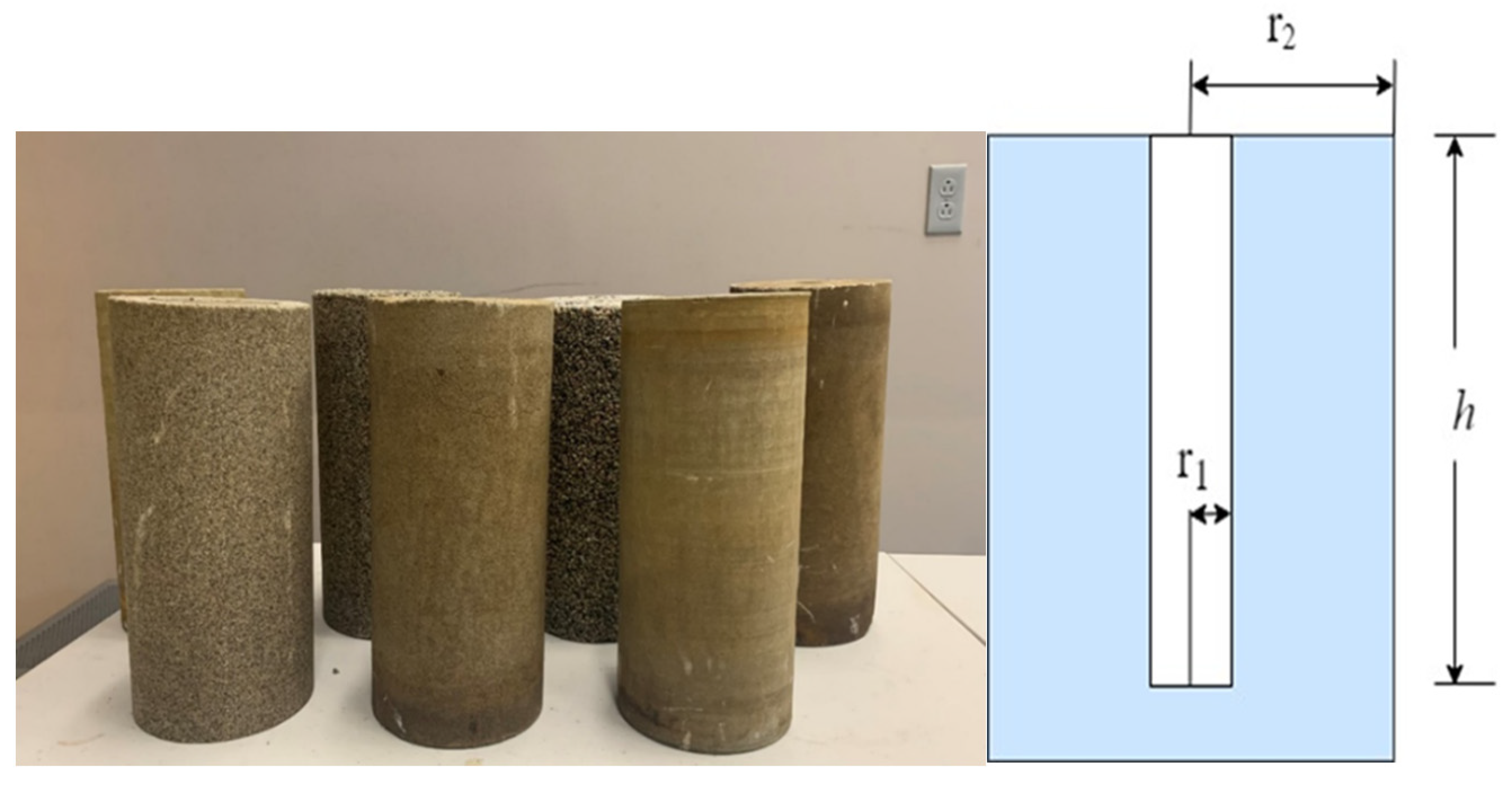
The experimental procedure was divided into two stages. The first stage is the preparation of samples from sandstone and epoxy. The second is conducting flow experiments on the Radial Flow Cell Facility. The experimental process is briefly described as follows. Initially, the experiments started at a low flow rate, and then the flow rate increased until the non-Darcy flow occurred. The air compressor has a large flow rate and continuously works for an extended period. High-velocity flow experiments have been performed on artificial samples to simulate the airflow in the near-wellbore region. The samples are cylindrical with 15.54 cm in diameter, and the perforation has a 25.54 depth and 2.54 cm in diameter, as shown in Figure 1.
3.1. Preparation of the Samples
Seven artificial samples were created in memorial University laboratories. Both Aziz and Ahmed et al. [44] made samples in the labs to produce samples using sand and epoxy. Lately, seven synthetic sand samples were created from sand collected from Nova Scotia Canada in the Memorial University of Newfoundland laboratory. The sand was dried in the civil engineering lab using a hot-air oven at 110 C. The sieving process resulted in six different sand sizes ranging from 0.18 mm to 1.18 mm. The sand at different sizes is mixed with epoxy at different quantities. The mixture is then placed in a plastic container throughout four stages, using an electric vibrator to ensure grain distribution with the epoxy glue, and then they lift to dry and consolidate for 24 h, as shown in Figure 1. The sample dimensions are 30.48 cm high, 15.54 cm diameter, and a perforation tunnel has a 25.54 cm depth and 2.54 cm diameter Abobaker et al. [45].
There are many available ways to measure the properties of the samples. Mercury Intrusion Porosimetry (MIP) is one of the most widely used ways at the University of Memorial of Newfoundland labs to characterize and analyze the synthetic samples’ pore morphology and index properties. The index properties include permeability, porosity, median pore diameter, and tortuosity, which are listed in the following Table 2.
3.2. Performing the Flow Experiments
At this stage, seven sandstone samples were prepared; the next step is to conduct the flow experiments. RFC Figure 2 Ahamed et al. [44] has been updated to be suitable for conducting multi-phase flow experiments, as five pressure sensors have been calibrated with pressure sensors from other experiments. Two pressure sensors were placed on the inlet and outlet, and the rest was placed on the fluid mixing lines. With help from the university’s technical department, an air flowmeter was repaired and successfully calibrated. In addition, another two lines were added to make the experiment ready to perform experiments on a three-phase flow. The experiment procedure begins by placing the sample in the cylinder and connecting the air compressor with the injection lines. The pressure sensors and flow meters are connected to the data acquisition to monitor the flow rate and record the pressure data during the experiment. The airflow rate was ranged from 3 to 99 L per minute. The outlet inserted into the pack measured line pressures without end effects. Note that the flow was entering the sample radially direction of gas flow to avoid spurious readings due to gas impinging on or accelerating off the probes (pitot effects).
The experimental run starts by installing the sample in the samples chamber (12) (Figure 2) and then locking the lid tightly to prevent any leakage. The pressure sensors and the flowmeters are then connected to the Data Acquisition inlet, where each sensor has a specific channel. All the data for each run from the flowmeters and the pressure sensor were transferred to digital numbers and charts using Lab View. The flow starts by adjusting the air compressor at a certain pressure and putting the flow rate control valve at the needed flow rate. The flow enters the sample radially Figure 2; the outlet is installed at the top of the sample perforation. The flow rate range was between 3 and 99 LPM; at each run, the pressure and flow data are converted to an Excel table and then later analyzed.
4. Non-Darcy Flow Regime
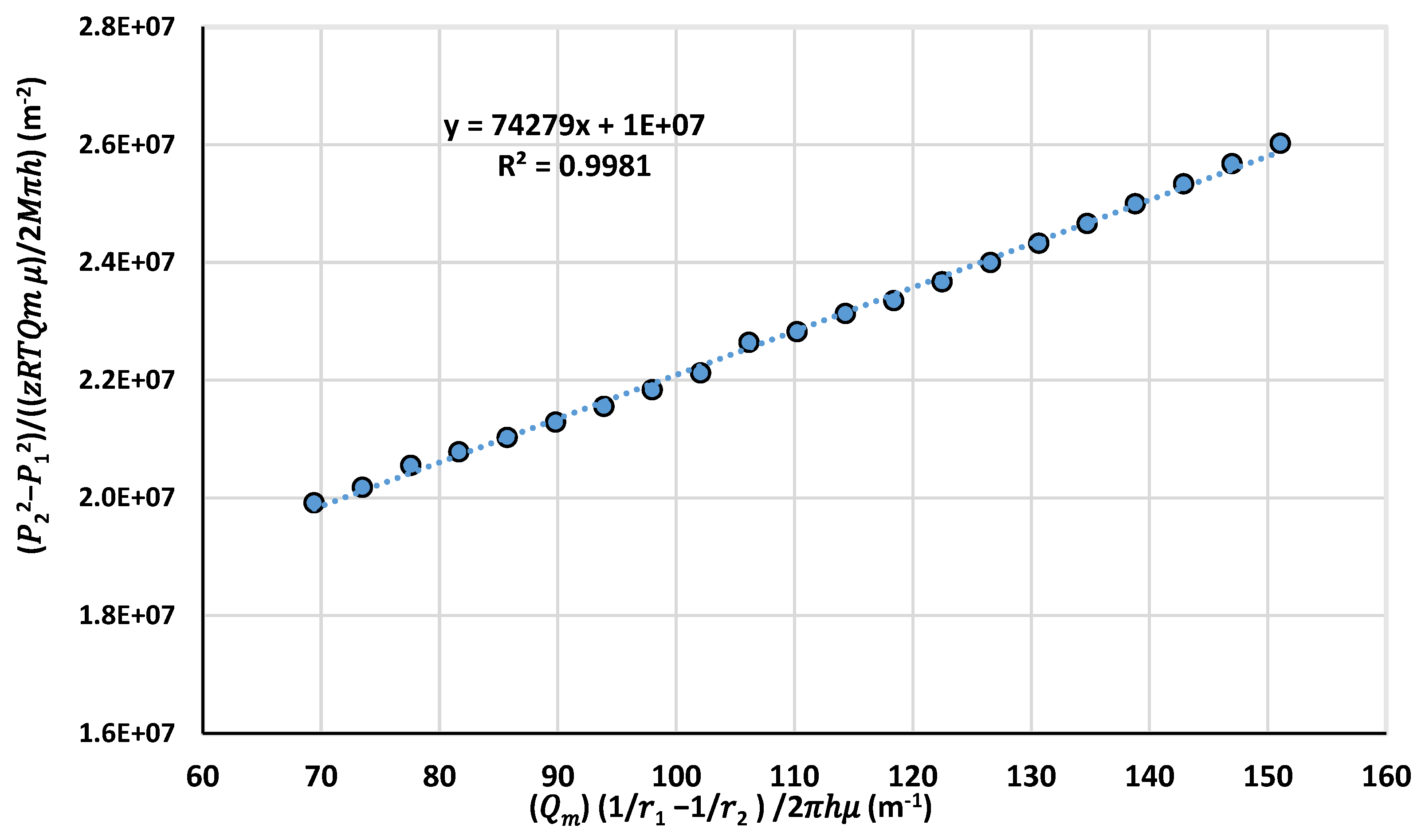
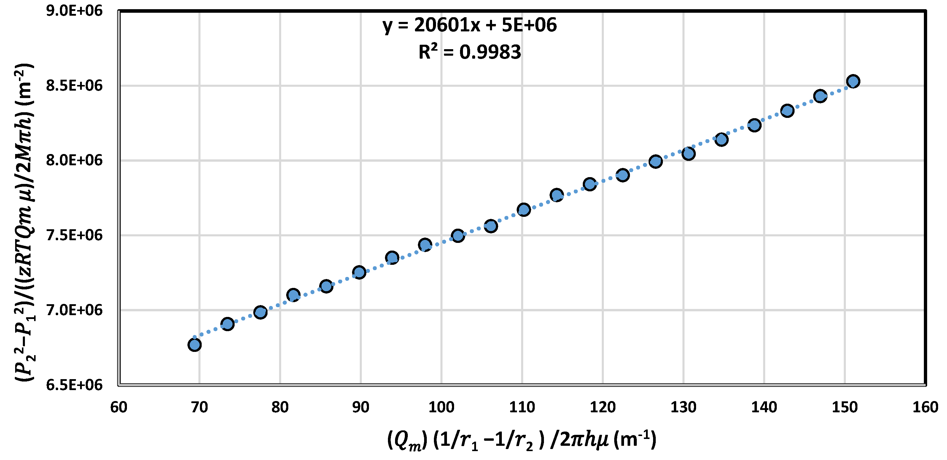
If Darcy’s law is considered assuming the air properties and k are constants and the term plotted versus () would create a straight line. Figure 3 and Figure 4 show the results of a test performed to check the nonlinearity of flow. By looking at Figure 3 and Figure 4, the lines are not straight, and this indicates the presence of non-Darcy flow. In fact, these lines can be described by equations of the second degree.
During the flow of air through the samples, a pressure loss occurs, which results in a decrease in the volumetric flow rate, but the mass flow rate remains constant. These changes in pressure and volumetric flow lead to a change in air properties such as density and viscosity.
4.1. Calculating Non-Darcy Coefficient β
A key to applying the Forchheimer Equation is to estimate a value for . Methods developed to calculate are based on experimental work, correlations, and the Forchheimer Equation. To determine () experimentally, the procedure is first to measure each of the core samples’ absolute permeability and then apply a series of increasing pressure differentials across each sample by flowing fluid through the core plugs at ever-increasing rates. Knowing the flow rates and pressure differentials across the sample, the inertial resistance coefficient can be directly calculated using linear regression of the Forchheimer Equation (8). Figure 5, Figure 6 and Figure 7 are the results of the flow experiments. The experimental data of () and were obtained in our Laboratory and utilized linear regression as in Figure 5, Figure 6 and Figure 7.
Table 3 contains the calculated values for the non-Darcy coefficient. The non-Darcy coefficient was compared with values obtained from models available in the literature. The closest result to the current study is Geertsma [27] model was the value of the difference is about 0.6 to 4.0%. It is clear from the table that there is a large discrepancy between the results obtained from this study and the results of previous studies. This discrepancy can be attributed to several reasons, the first of which is the size and nature of the samples. Studies use small samples during which the flow cannot reach full development. The other possible reason is that the current study benefits from the radial flow and the perforation, which is the outlet of the flow. As Zeng et al. [1] and others mentioned, the flow accelerates due to pressure differences when approaching the perforation, thus increasing the velocity and turbulence. The results obtained from the experiment were compared with previous studies in which the porous media used in those studies are similar to the samples of the current study.
4.2. Effect of Permeability, Porosity, Median Pore Diameter
Figure 8 reveals the variation of the non-Darcy according to the permeability from the modified Forchheimer plot of each sandstone sample. The plot illustrates the direct effect of permeability on the non-Darcy coefficient; with permeability increased, the non-Darcy coefficient decreases dramatically. These results show that the non-Darcy behavior is more severe in low permeability porous media. That can be explained as the pressure drop increases with the permeability decrease. Thus, the superficial velocity rises and leads to a more turbulent flow. The curvature of the aspect of decline is definite by increased permeability. Some previous studies proposed defining the equation of the non-Darcy coefficient with permeability. They attempted linear regression analysis on the experimental data set of the coefficient despite the curvature noted of transition [27].
It can be seen from Figure 9 that the non-Darcy coefficient decreases with the increase of median pore diameter. The non-Darcy coefficient decreases slowly in the bigger pore diameters, and that is because the flow cross-section area is larger in the porous media with a large pore.
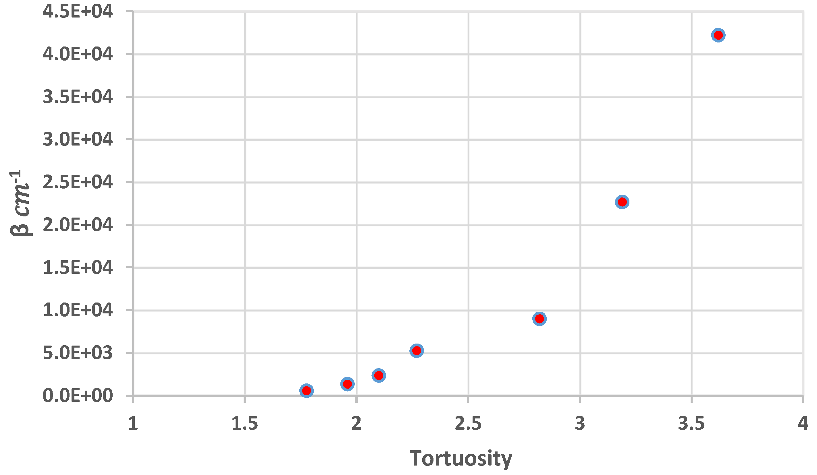
Figure 10 shows the non-Darcy coefficient versus the tortuosity of the samples. The graphs indicate that the non-Darcy coefficient is directly proportional to the tortuosity. The non-Darcy coefficient increases with the increase in tortuosity.
4.3. Forchheimer Number
Forchheimer number , which is used instead of the Reynolds number, which indicates when nonlinear effects occur, is given as the following:
where is the Darcy velocity, the superficial velocity. for the sample is calculated for each flow rate as follows: Assuming there is no loss of air in the flow system due to leakage, reaction, or any other reasons, the mass flow rate in the air compressor is the same as that in the core sample at flow equilibrium, though the volumetric flow rates can be different due to the change in pressures. On the other hand, the mass flow rate equals the product of the density and the volumetric flow rate. Similar to the calculation of and , the density of air in the sample is calculated using the pressure data [1]. This behavior implies that the superficial velocity alone, as in the Reynolds number, is not a criterion for identifying the non-Darcy flow behavior; therefore, the Forchheimer number can be calculated.
By analyzing the values in Table 4, it is observed that increases nonlinearly with the increase in the flow rate, which is a natural result of increasing the velocity leads to an increase in the nonlinearity. The nonlinearity increases in the indicate that the superficial velocity is not the only reason. However, interestingly, when comparing with permeability, it is noticed that the divergence in values is greater with the increase in permeability values at the same velocity. That conclusion is consistent with the fact that the non-Darcy behavior is more severe in low permeability porous media.
5. Conclusions
- This study conducted a radial flow experiment to investigate the existence of non-Darcy flow and calculate the non-Darcy “inertia” coefficient. Seven artificial samples were used. The flow rate of the air ranged from 3 LPM to 99 LPM, and in total, 231 run were conducted.
- Using the mean of pressure square difference versus plot the non-Darcy behavior was conformed. This resulted in lines better fit to a polynomial.
- The non-Darcy coefficient β was calculated for each sample from the experimental results of the pressure gradient and using linear regression. The β measurement results were between 276,180.32 and 19,589.15 .
- The non-Darcy coefficient decreases with the increase in the median pore diameter and the porosity. When the median pore diameter at 25.31 µm non-Darcy coefficient β 276,180.32 and at median pore diameter 181 µm non-Darcy coefficient β = 19,589.15 .
- Forchheimer numbers for airflow at varied flow rates are determined using experimental permeability and non-Darcy coefficient data.
Author Contributions
Conceptualization, A.E.; methodology, A.E.; software, A.E. and E.A.; validation, A.E.; formal analysis, A.E.; investigation, A.E.; data curation, A.E., E.A. and A.A.; writing—original draft preparation, A.E.; writing—review and editing, A.E., E.A., F.K., A.A.; supervision, F.K., M.A.R., A.A.; project administration S.D.B.; funding acquisition, M.A.R. All authors have read and agreed to the published version of the manuscript.
Funding
Qatar National Research Fund (a member of the Qatar Foundation).
Institutional Review Board Statement
Not applicable.
Informed Consent Statement
Not applicable.
Data Availability Statement
All data are contained within the article.
Acknowledgments
This publication was made possible by grant NPRP10-0101-170091 from the Qatar National Research Fund (a member of the Qatar Foundation).
Conflicts of Interest
The authors declare no conflict of interest.
Nomenclature
| flow area, | |
| zRT/M, J | |
| molecular weight | |
| pressure, Pa | |
| volumetric flow rate, | |
| mass flow rate, kg | |
| temperature, K | |
| seepage velocity, Darcy’s velocity, m | |
| fluid velocity, superficial velocity, m | |
| compressibility coefficient | |
| non-Darcy flow coefficient, | |
| porosity, adimensional | |
| fluid viscosity, Pa s | |
| fluid density, kg | |
| air density at the air compressor | |
| volumetric flow rate |
References
- Zeng, Z.; Grigg, R. A Criterion for Non-Darcy Flow in Porous Media. Transp. Porous Media 2006, 63, 57–69. [Google Scholar] [CrossRef]
- Whitaker, S. Advances in theory of fluid motion in porous media. Ind. Eng. Chem. 1969, 61, 14–28. [Google Scholar] [CrossRef]
- Hassnizadeh, M.; Gray, W. General conservation equations for multi-phase systems: 1. Averaging procedure. Adv. Water Resour. 1979, 2, 131–144. [Google Scholar] [CrossRef]
- Green, C.T.; Stonestrom, D.A.; Bekins, B.A.; Akstin, K.C.; Schulz, M.S. Percolation and transport in a sandy soil under a natural hydraulic gradient. Water Resour. Res. 2005, 41. [Google Scholar] [CrossRef] [Green Version]
- Forchheimer, P. Wasserbewegung durch Boden. Z. Ver. Dtsch. Ing. 1901, 45, 1781–1788. [Google Scholar]
- Kadi, K.S. Non-Darcy Flow In Dissolved Gas-Drive Reservoirs. In Proceedings of the SPE Annual Technical Conference and Exhibition, Dallas, TX, USA, 24–27 September 1980. [Google Scholar]
- Belhaj, H.; Agha, K.; Nouri, A.; Butt, S.; Vaziri, H.; Islam, M.R. Numerical Modeling of Forchheimer’s Equation to Describe Darcy and Non-Darcy Flow in Porous Media. In Proceedings of the SPE Asia Pacific Oil and Gas Conference and Exhibition, Jakarta, Indonesia, 9–11 September 2003. [Google Scholar]
- Rushing, J.; Newsham, K.; Fraassen, K.V. Measurement of the Two-Phase Gas Slippage Phenomenon and Its Effect on Gas Relative Permeability in Tight Gas Sands. In Proceedings of the SPE Annual Technical Conference and Exhibition, Denver, CO, USA, 5–8 October 2003. [Google Scholar]
- Katz, D.; Cornell, D.; Vary, J.; Kobayashi, R. Handbook of Natural Gas Engineering; Mcgraw-Hill Book Company: New York, NY, USA, 1959. [Google Scholar]
- Holditch, S.A.; Morse, R.A. The Effects of Non-Darcy Flow on the Behavior of Hydraulically Fractured Gas Wells. J. Pet. Technol. 1979, 28, 1169–1179. [Google Scholar] [CrossRef]
- Guppy, K.H.; Cinco-Ley, H.; Ramey, H.J. Pressure buildup analysis of fractured wells producing at high flowrates. J. Pet. Technol. 1982, 34, 2656–2666. [Google Scholar] [CrossRef]
- Martins, J.P.; Milton-Tayler, D.; Leung, H.K. The Effects of Non-Darcy Flow in Propped Hydraulic Fractures. In Proceedings of the SPE Annual Technical Conference and Exhibition, New Orleans, LA, USA, 23–26 September 1990. [Google Scholar]
- David, C.; Donald, K. An analysis of high-velocity gas flow through porous media. Ind. Eng. Chem. 1953, 10, 2145–2152. [Google Scholar]
- Shiri, Y.; Hassani, H. Two-component Fluid Front Tracking in Fault Zone and Discontinuity with Permeability Heterogeneity. Rud. -Geol. -Naft. Zb. 2021, 36, 19–30. [Google Scholar] [CrossRef]
- Shiri, Y.; Shiri, A. Numerical Investigation of Fluid Flow Instabilities in Pore-Scale with Heterogeneities in Permeability and Wettability. Rud. -Geol. -Naft. Zb. 2021, 36, 143–156. [Google Scholar] [CrossRef]
- Faez, M.; Ramezanzadeh, A.; Ghavami-Riabi, R.; Tokhmechi, B. The evaluation of the effect of fracture geometry on permeability based on laboratory study and numerical modelling. Rud. -Geol. -Naft. Zb. 2021, 36, 155–164. [Google Scholar] [CrossRef]
- Namdari, S.; Baghbanan, A.; Hashemolhosseini, H. Investigation of the effect of the discontinuity direction on fluid flow in porous rock masses on a large-scale using hybrid FVM-DFN and streamline simulation. Rud. -Geol. -Naft. Zb. 2021, 36, 49–59. [Google Scholar] [CrossRef]
- Ergun, S. Fluid flow through packed column. Chem. Eng. Prog. 1952, 48, 89–94. [Google Scholar]
- John, J.; Donald, K. Applications of unsteady state gas flow calculations. In Proceedings of the Research Conference “Flow of Natural Gas from Reservoirs”, Ann Arbor, MI, USA, 30 June–1 July 1955. [Google Scholar]
- Cooke, C.J. Conductivity of Fracture Proppants in Multiple Layers. J. Pet. Technol. 1973, 25, 1101–1107. [Google Scholar] [CrossRef]
- Macdonald, I.F.; El-Sayed, M.S.; Mow, K.; Dullien, F.A.L. Flow through Porous Media—The Ergun Equation Revisited. Ind. Eng. Chem. Fundam. 1979, 18, 199–208. [Google Scholar] [CrossRef]
- Kutasov, I.M. Equation Predicts Non-Darcy Flow Coefficient. Oil Gas J. 1993, 91, 66–67. [Google Scholar]
- Liu, X.; Civan, F.; Evans, R. Correlation of the Non-Darcy Flow Coefficient. J. Can. Pet. Technol. 1995, 34, PETSOC-95-10-05. [Google Scholar] [CrossRef]
- Coles, M.E.; Hartman, K.J. Non-Darcy Measurements in Dry Core and the Effect of Immobile Liquid. In Proceedings of the SPE Gas Technology Symposium, Calgary, AB, Canada, 15–18 March 1998. [Google Scholar]
- Pascal, H.; Quillian, R.G. Analysis Of Vertical Fracture Length And Non-Darcy Flow Coefficient Using Variable Rate Tests. In Proceedings of the SPE Annual Technical Conference and Exhibition, Dallas, TX, USA, 24–27 September 1980. [Google Scholar]
- Cornell, D.; Katz, D.L. Flow of Gases through Consolidated Porous Media. Ind. Eng. Chem. 1953, 45, 2145–2152. [Google Scholar] [CrossRef]
- Geertsma, J. Estimating the Coefficient of Inertial Resistance in Fluid Flow Through Porous Media. Soc. Pet. Eng. J. 1974, 14, 445–450. [Google Scholar] [CrossRef]
- Evans, E.; Evans, R. Influence of an Immobile or Mobile Saturation on Non-Darcy Compressible Flow of Real Gases in Propped Fractures. J. Pet. Technol. 1988, 40, 1345–1351. [Google Scholar] [CrossRef]
- Whitney, D.D. Characterization of the Non-Darcy Flow Coefficient in Propped Hydraulic Fractures. Master’s Thesis, University of Oklahoma, Norman, OK, USA, 1988. [Google Scholar]
- Li, D. Analytical Study of the Wafer Non-Darcy Flow Experiments. In Proceedings of the SPE Western Regional/AAPG Pacific Section Joint Meeting, Anchorage, AK, USA, 8–10 May 2002. [Google Scholar]
- Tek, M.R.; Coats, K.H.; Katz, D.L. Turbulence on Flow of Natural Gas Through Porous Reservoirs. J. Pet. Technol. 1962, 14, 799–806. [Google Scholar] [CrossRef]
- Yao, Y.; Li, G.; Qin, P. Seepage features of high-velocity non-Darcy flow in highly productive reservoirs. J. Nat. Gas Sci. Eng. 2015, 27, 1732–1738. [Google Scholar] [CrossRef]
- Core, J. Using the Inertial Coefficient, B, To Characterize Heterogeneity in Reservoir Rock. In Proceedings of the SPE Annual Technical Conference and Exhibition, Dallas, TX, USA, 27–30 September 1987. [Google Scholar]
- Li, D.; Svec, R.K.; Engler, T.W.; Grigg, R.B. Modeling and Simulation of the Wafer Non-Darcy Flow Experiments. In Proceedings of the SPE Western Regional Meeting, Bakersfield, CA, USA, 8–10 March 2001. [Google Scholar]
- Thauvin, F.; Mohanty, K.K. Network Modeling of Non-Darcy Flow Through Porous Media. Transp. Porous Media 1998, 31, 19–37. [Google Scholar] [CrossRef]
- Shachi, S.; Yadav, B.K.; Rahman, M.A.; Pal, M. Migration of CO2 through Carbonate Cores: Effect of Salinity, Pressure, and Cyclic Brine-CO2 Injection. J. Environ. Eng. 2020, 146, 04019114. [Google Scholar] [CrossRef]
- Ahammad, M.J.; Alam, J.; Rahman, M.; Butt, S.D. Numerical simulation of two-phase flow in porous media using a wavelet based phase-field method. Chem. Eng. Sci. 2017, 173, 230–241. [Google Scholar] [CrossRef]
- Sajjad Rabbani, H.; Osman, Y.; Almaghrabi, I.; Azizur Rahman, M.; Seers, T. The Control of Apparent Wettability on the Efficiency of Surfactant Flooding in Tight Carbonate Rocks. Processes 2019, 7, 684. [Google Scholar] [CrossRef] [Green Version]
- Ding, L.; Cui, L.; Jouenne, S.; Gharbi, O.; Pal, M.; Bertin, H.; Rahman, M.A.; Romero, C.; Guérillot, D. Estimation of Local Equilibrium Model Parameters for Simulation of the Laboratory Foam-Enhanced Oil Recovery Process Using a Commercial Reservoir Simulator. ACS Omega 2020, 5, 23437–23449. [Google Scholar] [CrossRef]
- Rahman, M.; Mustafiz, S.; Koksal, M.; Islam, M. Quantifying the skin factor for estimating the completion efficiency of perforation tunnels in petroleum wells. J. Pet. Sci. Eng. 2007, 58, 99–110. [Google Scholar] [CrossRef]
- Rahman, M.; Mustafiz, S.; Biazar, J.; Koksal, M.; Islam, M. Investigation of a novel perforation technique in petroleum wells—Perforation by drilling. J. Frankl. Inst. 2007, 344, 777–789. [Google Scholar] [CrossRef]
- Zheng, L.; Rahman, M.; Ahammad, M.J.; Butt, S.D.; Alam, J. Experimental and Numerical Investigation of a Novel Technique for Perforation in Petroleum Reservoir. In Proceedings of the SPE International Conference and Exhibition on Formation Damage Control, Lafayette, LA, USA, 19–21 February 2016. [Google Scholar] [CrossRef]
- Abobaker, E.; Elsanoose, A.; Khan, F.; Rahman, M.A.; Aborig, A.; Noah, K. A New Evaluation of Skin Factor in Inclined Wells with Anisotropic Permeability. Energies 2021, 14, 5585. [Google Scholar] [CrossRef]
- Ahammad, J.; Rahman, A.; Butt, S.; Alam, M. An Experimental Development to Characterise the Flow Phenomena at the Near-Wellbore Region. In Proceedings of the ASME 2019 38th International Conference on Ocean, Offshore and Arctic Engineering, Glasgow, UK, 9–14 June 2019. [Google Scholar]
- Abobaker, E.; Elsanoose, A.; Rahman, M.A.; Aborig, A.; Zhang, Y.; Sripal, E. Investigation-the-Effect-Mixing-Grain-Size-and-Epoxy-Glue-Content-on-Index-Properties-of-Synthetic-Sandstone-Sample. In Proceedings of the Canadian Society for Mechanical Engineering International Congress, Charlottetown, PE, Canada, 21–24 June 2020. [Google Scholar]
Figure 1.
Seven artificial samples.

Figure 2.
Schematic diagram of the experiment RFC facility: 1. Sample, 2. Inlet, 3. Outlet, 4. Pressure Sensors, 5. Water pump, 6. Air compressor, 7. non-Return valves, 8. Airflow meter, 9. Water flowmeter, 10. Data Acquisition, 11. Computer, 12. Samples Chamber, 13. Waterline.
Figure 2.
Schematic diagram of the experiment RFC facility: 1. Sample, 2. Inlet, 3. Outlet, 4. Pressure Sensors, 5. Water pump, 6. Air compressor, 7. non-Return valves, 8. Airflow meter, 9. Water flowmeter, 10. Data Acquisition, 11. Computer, 12. Samples Chamber, 13. Waterline.

Figure 3.
Nonlinearity of Darcy flow check of the samples 1, 2, and 3.

Figure 4.
Nonlinearity of Darcy flow check of the samples 4, 5, and 6.

Figure 5.
Calculating the non-Darcy β. Permeability = 2, Darcy.

Figure 6.
Calculating the non-Darcy β. Permeability = 12 Darcy.

Figure 7.
Calculating the non-Darcy β. Permeability = 26 Darcy.

Figure 8.
The effect of permeability inertia coefficient β.

Figure 9.
The effect of Median pore diameter on inertia coefficient β.

Figure 10.
The effect of tortuosity on inertia coefficient β.

Table 2.
Properties for the samples.
| Sample No. | The Index Properties for the Samples | |||
|---|---|---|---|---|
| Permeability (mD) | Porosity (%) | Tortuosity | MPD (µm) | |
| Sample 1 | 2035.95 | 33 | 3.62 | 25.31 |
| Sample 2 | 3981.50 | 29.23 | 3.19 | 32.14 |
| Sample 3 | 6292.66 | 27 | 2.82 | 45.27 |
| Sample 4 | 8127.04 | 26.6 | 2.27 | 60.6101 |
| Sample 5 | 12,281.50 | 25.8 | 2.10 | 81 |
| Sample 6 | 16,320.24 | 25.5 | 1.96 | 100 |
| Sample 7 | 26,151.72 | 25 | 1.7765 | 181.7485 |
Table 3.
Calculated values for non-Darcy’s coefficient.
| Sample No | Geertsma [27] | Tek [31] | |
|---|---|---|---|
| Sample 1 | 276,180.32 | 440,041.83 | 14,556.91 |
| Sample 2 | 210,821.61 | 153,871.68 | 5708.06 |
| Sample 3 | 169,710.87 | 122,395.33 | 2954.77 |
| Sample 4 | 119,204.17 | 29,141.28 | 1957.57 |
| Sample 5 | 73,103.274 | 17,068.78 | 1117.16 |
| Sample 6 | 38,663.54 | 10,077.68 | 742.99 |
| Sample 7 | 19,589.15 | 4165.19 | 377.27 |
Table 4.
Forchheimer number .
| Q LPM/s | Sample 3 | Sample 4 | Sample 5 | Sample 7 |
|---|---|---|---|---|
| 3 | 0.0682 | 0.0573 | 0.0124 | 0.0073 |
| 9 | 0.2041 | 0.1708 | 0.0369 | 0.0146 |
| 15 | 0.3389 | 0.2829 | 0.0613 | 0.0218 |
| 21 | 0.4729 | 0.3938 | 0.0854 | 0.0291 |
| 27 | 0.606 | 0.5033 | 0.1093 | 0.0362 |
| 33 | 0.738 | 0.6116 | 0.1329 | 0.0434 |
| 39 | 0.869 | 0.7185 | 0.1564 | 0.0506 |
| 45 | 1.000 | 0.8243 | 0.1797 | 0.0578 |
| 51 | 1.129 | 0.9288 | 0.2027 | 0.0649 |
| 57 | 1.258 | 1.032 | 0.2256 | 0.0720 |
| 63 | 1.386 | 1.134 | 0.2483 | 0.0791 |
| 69 | 1.512 | 1.235 | 0.2707 | 0.0862 |
| 75 | 1.638 | 1.335 | 0.2929 | 0.0932 |
| 81 | 1.764 | 1.434 | 0.3150 | 0.1003 |
| 87 | 1.888 | 1.531 | 0.3369 | 0.1073 |
| 93 | 2.0116 | 1.628 | 0.3586 | 0.1143 |
| 99 | 2.1344 | 1.723 | 0.3801 | 0.1213 |
Publisher’s Note: MDPI stays neutral with regard to jurisdictional claims in published maps and institutional affiliations. |
© 2022 by the authors. Licensee MDPI, Basel, Switzerland. This article is an open access article distributed under the terms and conditions of the Creative Commons Attribution (CC BY) license (https://creativecommons.org/licenses/by/4.0/).
Share and Cite
MDPI and ACS Style
Elsanoose, A.; Abobaker, E.; Khan, F.; Rahman, M.A.; Aborig, A.; Butt, S.D. Estimating of Non-Darcy Flow Coefficient in Artificial Porous Media. Energies 2022, 15, 1197. https://doi.org/10.3390/en15031197
AMA Style
Elsanoose A, Abobaker E, Khan F, Rahman MA, Aborig A, Butt SD. Estimating of Non-Darcy Flow Coefficient in Artificial Porous Media. Energies. 2022; 15(3):1197. https://doi.org/10.3390/en15031197
Chicago/Turabian StyleElsanoose, Abadelhalim, Ekhwaiter Abobaker, Faisal Khan, Mohammad Azizur Rahman, Amer Aborig, and Stephen D. Butt. 2022. "Estimating of Non-Darcy Flow Coefficient in Artificial Porous Media" Energies 15, no. 3: 1197. https://doi.org/10.3390/en15031197
Note that from the first issue of 2016, this journal uses article numbers instead of page numbers. See further details here.