
Possibility to Use Professional Bicycle Computers for the Scientific Evaluation of Electric Bikes: Trajectory, Distance, and Slope Data


Department of Road Transport, Faculty of Transport and Aviation Engineering, Silesian University of Technology, 8 Krasinskiego Street, 40-019 Katowice, Poland
*
Authors to whom correspondence should be addressed.
Energies 2022, 15(3), 758; https://doi.org/10.3390/en15030758
Submission received: 25 December 2021
/
Revised: 18 January 2022
/
Accepted: 19 January 2022
/
Published: 20 January 2022
(This article belongs to the Special Issue Electric and Hybrid Vehicles: Technology Trends, Challenges and Opportunities)
Abstract
:This work presents an analysis of data recorded by a bicycle computer paired with typical measurement sensors in order to determine whether the data can be useful for a scientific evaluation of the cyclist–electric bicycle anthropotechnical system. There are no studies on this subject in the available literature. An attempt was made to estimate the quality of data and define the most effective methods of processing and filtering. The imperfections of the measurement system and the potential directions of the development of bicycle computers are indicated. Particular attention has been given to the data needed to compare the energy efficiency of assisted electric bicycles. However, the results of the analyses can also be used in cyclist endurance tests and to simulate routes in various types of bicycle trainers. The article focuses on the data obtained from the GPS module and the barometric altimeter, which make it possible to estimate the trajectory of movement, the distance traveled, and the height of the route above sea level as well as its slope. In order to assess the accuracy, the data from the bicycle computer was compared with the geodetic data. Methods for averaging GPS routes were also proposed. In this way, it was possible to identify the parameters of the selected path for testing bicycles quite accurately. The research presented in this paper is an introduction to the development of methods for assessing the energy efficiency of electric bicycles. Analyses of other data measured by the cycling computer, such as speed, cadence, and power, will be carried out in the second planned part of the article.
1. Introduction
The last decade has seen a dynamic technological development of bicycle computers, which are evolving toward on-board computers equipped with a GPS receiver, data recorder, and the ability to communicate with many sensors tracking important parameters of the bicycle’s movement and the cyclist’s efficiency.
As standard, the bicycle computer has a built-in GPS module, a barometric altimeter, and often a thermometer. Using Bluetooth/ANT + communication, the computer easily connects wirelessly with sensors: speed, cadence, pedal force, pedal power, pulse, etc., from which it downloads and archives data. Linking the data from sensors together with the distance traveled and time greatly facilitates their subsequent analysis in various terms e.g., good driving technique. Thanks to the far-reaching miniaturization, both the bicycle computer and additional measurement sensors practically do not change the riding conditions. These devices also have a very low energy requirement and run for hours without recharging. In selected speed, cadence, and heart rate sensors, the battery is replaced at intervals counted in months. A possible disadvantage of such systems is the very difficult access to information on the measurement data processing methods used in them and technical documentation in general.
Currently, there are more and more scientific papers on the use of bicycle computers and smartphones in scientific research and in competitive sports e.g., works [1,2,3].
For example, in order to carry out comparative energy efficiency studies of electric and conventional bicycles, reliable data on the distance traveled, route gradient, speed, cadence, and power must be available. In addition, such data may be needed to analyze a cyclist’s performance or to build bicycle trainers recreating real conditions [4].
The inspiration for the research carried out in the work was a completely different problem: the assessment of the energy efficiency of electric bicycles. Comparing the energy efficiency of bicycles required choosing a test route and good identification of its parameters. The second task was to collect the data necessary to perform the energy balance of the bicycles. The authors asked themselves: is it possible to use a bicycle computer for this purpose?
The paper presents a critical assessment of the quality of parameters recorded by a modern bicycle computer made by one of the leading manufacturers. The aim of the research was to determine whether the recorded signals are precise enough to be used for the broadly understood scientific evaluation of the cyclist–bicycle anthropotechnical system. There are no examples in the literature for assessing the quality of data recorded by bicycle computers. The exception is the work in which algorithms were analyzed to determine pedaling efficiency and power uniformity [5]. The authors hope that the presented article and the planned second part of it will fill this gap.
The bicycle computer used for the research recorded at a frequency of 1 Hz parameters such as speed according to the speed sensor mounted in the bicycle wheel, speed according to GPS, GPS position, cadence, temperature, power, and uniformity of power distribution (right/left pedal). This article discusses only part of the research results, focusing on data obtained from the GPS system and the barometric altimeter. Other research results concerning, among others, speed, cadence, and power measurements will be presented in the next part of the article.
GPS data (geodetic latitude and longitude in WGS84) are usually noisy due to the sensitivity of the tracking system and therefore are inaccurate [6]. Many factors, such as driving in forests, mountainous terrain, near tall buildings, also tropospheric conditions, or sun activities, may cause errors or loss of satellite signal. GPS trajectories due to errors and missing data often require appropriate pre-processing before their application [7]. For example, for the smoothing and filtering of GPS data, the Kalman filter can be used [8,9,10]. The bicycle computer saves GPS data every 1 s. This recording rate seems too low, because the bike can cover a distance of several meters at the time. However, it can be presumed that saved data are early properly filtered, interpolated, and smoothed. A typical GPS unit reads a position with frequency between 1 and 5 Hz; newer units reach frequencies of 10–15 Hz [11]. There is an ongoing discussion on the optimal frequency of the GPS unit [12].
2. Materials and Methods
2.1. Materials: Electric Bike and Measuring Equipment
Four different bicycles, including two electrically assisted bicycles, were used to conduct the tests (electric bicycles are shown in Figure 1). The main purpose of the tests was the energy assessment of bicycles; the problem of assessing the quality of data recorded by the bicycle computer appeared along the way. The route was always traveled by the same cyclist. He used the various assist modes available when riding e-bikes. After the test, the electric bike batteries were not recharged, but it can be assumed that due to the short distance (≈2.6 km) and slight difference in elevation (≈25 m), the effectiveness of the assistance did not decrease significantly. The same cycle computer was installed before each bicycle trial. In addition, a set for measuring the power in the pedals and additionally, for selected bikes, speed and cadence sensors were installed on the bikes. The measurement kit included a bicycle computer ELEMNT ROAM (Figure 2), Wahoo CADENCE, Wahoo SPEED, TICKR, and Look Exact Dual Pedals system.
2.2. Materials: Test Route
All travel tests were carried out on the same route with a length of just over 2.6 km in the form of a closed loop, as shown in Figure 3. The route included asphalt and gravel (about 200 m at the start–finish) sections, two sharp turns, and a long driveway with a level difference of almost 35 m. Local traffic during the tests was minimal and did not interfere with their course. There were no natural or artificial objects on the route that could interfere with the GPS signal.
2.3. Methods: Trials
Several trials were carried out to travel a fixed route using traditional and electric bikes in various power assist modes and without assist. As a result, the obtained travel times differed significantly. This fact was important during further analyses of the recorded results. The selected analysis methods should be insensitive to differences in the lengths of the data series. The data from the bicycle computer were read and pre-evaluated. In one case, there were no GPS data at the start of the trial. In another, 36 s of all data was lost. Eight trials were selected for further analyses (Table 1), the data of which met the completeness criterion and at the same time differed in the number of recorded measurement points (which is equivalent to the travel time in seconds and meets the criterion of different series lengths).
In practice, it often happens that the averaged trajectory of the tract is sought, on which many trials have been made before. This case is also considered in this paper. The recorded trajectories differ mainly in the travel speed; therefore, the time series corresponding to them are of different lengths. The differences in the shape of the trajectory results from the fact that parts of the route e.g., turns, could be overcome in various ways. The remaining fluctuations are probably due to the inaccuracies of the tracking system [13].
The problem of calculating an averaged route based on two or more routes can be solved in several ways. If the number of registered trajectories is small, the Dynamic Time Warping (DTW) method can be successfully used to compare and combine them [14]. In the case of a large number of trajectories, the methods of point clustering and averaging on the centroid principle can be used [15,16].
In time series analysis, DTW is one of the algorithms for measuring similarity between two temporal sequences, which may vary in speed. Dynamic time warping between two trajectories can be considered as a minimization of the cumulative distance between elements of two time series along searched path.
An example of using the DTW algorithm to determine the averaged path is shown in Figure 4. It is an enlarged fragment of the entire route. Before transforming, in order to increase the number of points on the trajectories, the signals from both trials were oversampled to 4 Hz using cubic interpolation.
To combine many trajectories, the hierarchical method proposed in [14] can be used (Figure 5). Hierarchical averaging is an effective method when the number of trajectories is not too large. At the same time, it is a labor-intensive method, and the workload increases with the number of trajectory points and number of examined trials. Ideally, the number of trials should be a power of 2 (). Then, the transformation should be performed.
A characteristic feature of the trajectories recorded by the bicycle computer is the uneven distribution of the points that create them. This is due to the different speed of the bicycle and is especially visible at the beginning and end of the trials. The DTW algorithm also transfers this feature to the averaged path.
The bicycle computer saves the distance information in a cumulative form (distance traveled). The algorithm by which the computer calculates the distance is not known. Technical information shows that in the event of problems with the GPS signal, the computer can use information from the speed sensor (if installed) to correct the position and distance traveled.
The distance between two points defined in GPS coordinates can be calculated using Haversine Formula (1), which determines the great-circle distance between two points on a sphere:
or equivalent Formula (2):
where atan2 is a function of MATLAB software.
To determine distance, the spherical law of cosines (SLC) is also used (3):
or equirectangular projection approximation (EPA) for small distances (4):
All angles must be in radians. is Earth’s radius, which can be taken equal to the mean radius of the WSG84 spheroid defined by the International Union of Geodesy and Geophysics as an arithmetic mean of the radii measured at two equator points and a pole ().
What is the effect of the radius value on the distance calculation? For example, the second so-called geocentric radius was selected. This radius is equal to the distance from the Earth’s center to a point of spheroid surface and can be calculated using Formula (5):
It should be noted that this radius does not coincide with the radii of curvature of the spheroid’s surface. At a latitude of degrees, this radius is equal [17].
Vincenty’s formulae [18] calculate the distance between two points on the surface of a spheroid and therefore should be more accurate. However, the calculations are very complex and are not applicable to distance calculations based on GPS data.
A real data test (trial 6) with double precision (64 bit) showed that the spherical law of cosines (SLC) gives relatively large errors compared to the Haversine formula. Equirectangular projection approximation (EPA) can be successfully used in place of the Haversine formula. The distances were calculated and compared for individual trajectory segments (Figure 6). In all Formulas (1)–(4), the distance depends linearly on the assumed radius of the Earth. Even though the sphere’s radii mean and geocentric differ by several thousand meters, the difference in distance is small. The relative error of the distance calculation will be less than one per mille (‰).
Trajectories recorded in GPS coordinates can be projected onto the map plane in rectangular coordinates. In Poland, for maps on a scale of 1:10,000 and smaller, the PUWG1992 (EPSG2180) reference system is used, based on the Gauss–Krüger conformal projection, with the central meridian 19°. The X-axis of the map plane is directed north, while the y-axis is directed east. The mapping parameters from WSG84 to PUWG 1992 are widely available. The authors prepared vectorized function, which transforms the entire trajectory in one call, based on [19].
The trial path covers the areas of two map sheets (scale 1:5000), respectively M-34-51-C-b-3-4 and M-34-51-C-b-4-3. Using the GEOPORTAL web application [20], it is possible to download a public orthophoto maps of these areas. An exemplary trajectory in the PUWG1992 coordinates against the background of orthophotos is shown in Figure 7. The visible imperfections result from the fact that the photo maps are saved in the tiff format and additionally differ slightly in resolution. The corresponding bitmaps must be appropriately scaled and fitted into the correct rectangular areas in the coordinate system.
The use of plane coordinates simplifies the calculation of distance, azimuth, etc. Unification the density of the points distribution on the trajectory, by introducing additional points at equal distances, is also easy. However, it should be noted that this is the distance traveled on the map plane and will differ from the actual distance calculated, for example, on the basis of the bicycle wheel rotation speed, especially when the route is steeply inclined.
2.4. Methods: Evaluation of Altitude and Slope Data
The bicycle computer used for the research calculates the altitude using information from two devices: a barometric altimeter and a GPS module. The basis is data from the barometric altimeter, which generally determines the change in altitude very accurately. A generally known formula is used for the altitude calculation (6):
where is the height depending on the pressure; , respectively, are the altitude, temperature, and pressure at the reference point; is the constant temperature gradient; and is the universal gas constant of air, the value of which also depends on the amount of water vapor in the dry air.
As can be seen, the barometric altimeter is very sensitive to changes in the reference temperature and to some extent to air humidity. A typical phenomenon is the so-called altimeter drift-altitude measurement error with slow pressure changes. The altimeter requires a reference height at the very beginning of the measurements and a continuous calibration to eliminate drift. For this purpose, the computer uses data from GPS [21]. However, the altitude readings from GPS have a large dispersion of values and therefore can be very inaccurate. The computer calibrates the altimeter data only after its internal algorithms confirm that the GPS altitude data are very likely to be true [22].
The accuracy of the bicycle computer to the route altitude and slope determination can be assessed using the Digital Terrain Model (DTM). For this purpose, the coordinates of the waypoints have to be linked to the corresponding height data. In Poland, such data are publicly available (system PL-KRON86-NH) and can be obtained from the government website [20]. The individual height data files correspond to the extent of the map sheets in rectangular planar PUWG1992 coordinates (on a scale of 1: 5000) and consist of text records in the format: (y_coord,x_coord,height). According to the information on the website, the height data were obtained thanks to laser scanning (LIDAR) with a resolution of a regular grid of 1 m × 1 m and a declared accuracy of 0.2 m. The text format of the files is inconvenient for computer processing, and it is best to transform it into a matrix form. The files contain only points that belong to the area on the surface of the ellipsoid before projection. For this reason, the obtained rectangular matrices do not contain height information at some points on the edges. Simultaneously, the sheets partially overlap. An example of a height map (DTM) created by joining sheets M-34-51-C-b-3-4 and M-34-51-C-b-4-3, which is intersected by the test route, is shown in Figure 8.
The altitude data provided are raw (and very noisy), as shown for the selected fragment of the 10 × 10 m map in Figure 9 (left). Although the differences in the height of adjacent points do not exceed the declared accuracy of the terrain projection, however, in order to be useful for further analysis, they should be processed. In the analyzed case, averaging was carried out with a filter with dimensions of 16 × 16 points (Figure 9 right). The position of each point on the trajectory in rectangular coordinates can now be referenced to the DTW regular grid, which allows you to calculate its height using Lagrange interpolation (Figure 10).
Knowing the altitude changes between two route points and the distance between them (distance traveled on the plane of the map), the computer can calculate the slope of the route (slope = rise/run). This parameter of the route is very important wherever the cyclist’s energy expenditure is analyzed. The computer gives the slope as a percentage. A 1% change in the slope, significant already in case of potential energy calculations, means a height difference of 1 cm per 1 m of the distance traveled. For this reason, the elevation data noise (data measured by computer) generates frequent fluctuations in the slope function depending on distance, especially when the terrain is flat. This effect is very difficult to eliminate. For example, for the smoothing of the slope function, averaging or median filtering can be used.
It is most obvious to use the method of forward difference for calculating the slope; then, the distance between adjacent points can be of any value. After re-sampling the height function e.g., by means of cubic interpolation, equidistant points can be obtained. Then, more complex numerical derivative methods such as center difference or five-point interpolation can be used.
2.5. Methods: Azimuth of Trajectory Segment
It is necessary to take into account the influence of the wind, as the azimuth of segments of the path a cyclist is riding on is an important parameter. The geographic azimuth can be determined in GPS coordinates from Formula (7):
where —start point, —end point of path segment, .
In the case of rectangular coordinates, the formula for the topographic azimuth is (8):
where —coordinates of ends of path segment.
Information about the wind direction can come from weather vane, which will probably be oriented with a compass. Corresponding corrections for the position of the reference meridian with respect to magnetic north should be taken into account in the calculations, as shown in Figure 11.
3. Results and Discussion
Eight recorded trajectories differing in travel time are combined in one averaged path using DTW and the hierarchical averaging method. A fragment of the averaged trajectory and trajectory from the trials are shown in Figure 12. As can be seen, the averaging method is very effective. Figure 13 compares the distances traveled in individual trials and the distance calculated for the averaged trajectory. Due to the different speed of travel in individual trials, only the total distance traveled can be compared with each other. The comparison of the length is just as good (red dotted line).
The resulting averaged path has been refined by eliminating points that are too close to each other and adding points where the distances between them are too great. The desired distance between adjacent track points is assumed to be approximately 0.5 m. Then, the GPS coordinates of the track points were converted to the rectangular coordinate system PUWG1992. The path obtained in this way was drawn against the background of the terrain height map (Figure 14).
Each point of the averaged trajectory in plane coordinates was assigned an appropriate height above sea level. The comparison of the trajectory heights recorded in individual trials and the trajectory height of the averaged path obtained from the geodetic data (DTM) are shown in Figure 15. It can be noted that the barometric altimeter shows changes in altitude very accurately, while the reference altitudes vary considerably. From the changes in altitude depending on the distance traveled, the slope of the route can be calculated. The calculations were made using various methods (Figure 16). As the differences are small, it is best to use the simplest method (forward difference), which does not require additional data re-sampling. The obtained graphs of the slope function are characterized by significant oscillations, and it is very difficult to assess whether it is the height data noise effect or the natural features of the terrain. Unfortunately, such a variation in the slope in real conditions is very likely.
The calculated slope function was re-sampled using cubic interpolation to obtain the same distance between successive points. Then, the data prepared in this way could be averaged with a median filter of the order of 64. The median filter, unlike the usual averaging filter, does not interfere so much with the results at the signal ends. Figure 17 shows the function of the averaged slope against the background of the slope determined by the forward difference. The comparison of the slopes recorded by the computer and the averaged slope determined on the basis of geodetic data is shown in Figure 18. Graphs of the slope functions calculated by the computer show large fluctuations, and it will be difficult to use them in further analyses. Perhaps the altimeter measurements are also influenced by vibrations generated while driving.
The slopes can be calculated independently from the registered height data. The functions of the slope from the distance travelled, calculated on the basis of the heights recorded in individual trials in relation to the averaged slope calculated on the basis of geodetic heights, are shown in Figure 19a,b. Slope functions without smoothing are shown Figure 19a. In Figure 19b, the functions were properly re-sampled, as described above, and then given to smoothing with a median filter. Since the interpolation algorithm requires the independent variable to be incremental and does not accept multiple nodes, the recorded data needed to be properly cleaned beforehand. Unfortunately, the result is still not very satisfactory, and the obtained functions are still not suitable for further analysis.
Determining the slope of the route based on geodetic data is quite precise but also time-consuming. Therefore, another attempt was made to obtain the slope function from the data recorded by the computer. This time, all of the data were first purified and sampled to vectors of the same length. As the distances in the individual trials differed slightly, this required not only interpolation but also extrapolation of the data at the ends. Then, all the slope functions from the eight trials were calculated, and mean values were determined. Finally, the resulting function was smoothed with the median filter. The result of the actions is shown in Figure 20. Good compliance of the slope function with that obtained from geodetic data was obtained. The method proposed above gives good results. The visible phase shift in the slope calculated from the test data may be caused by the drift of the barometric altimeter.
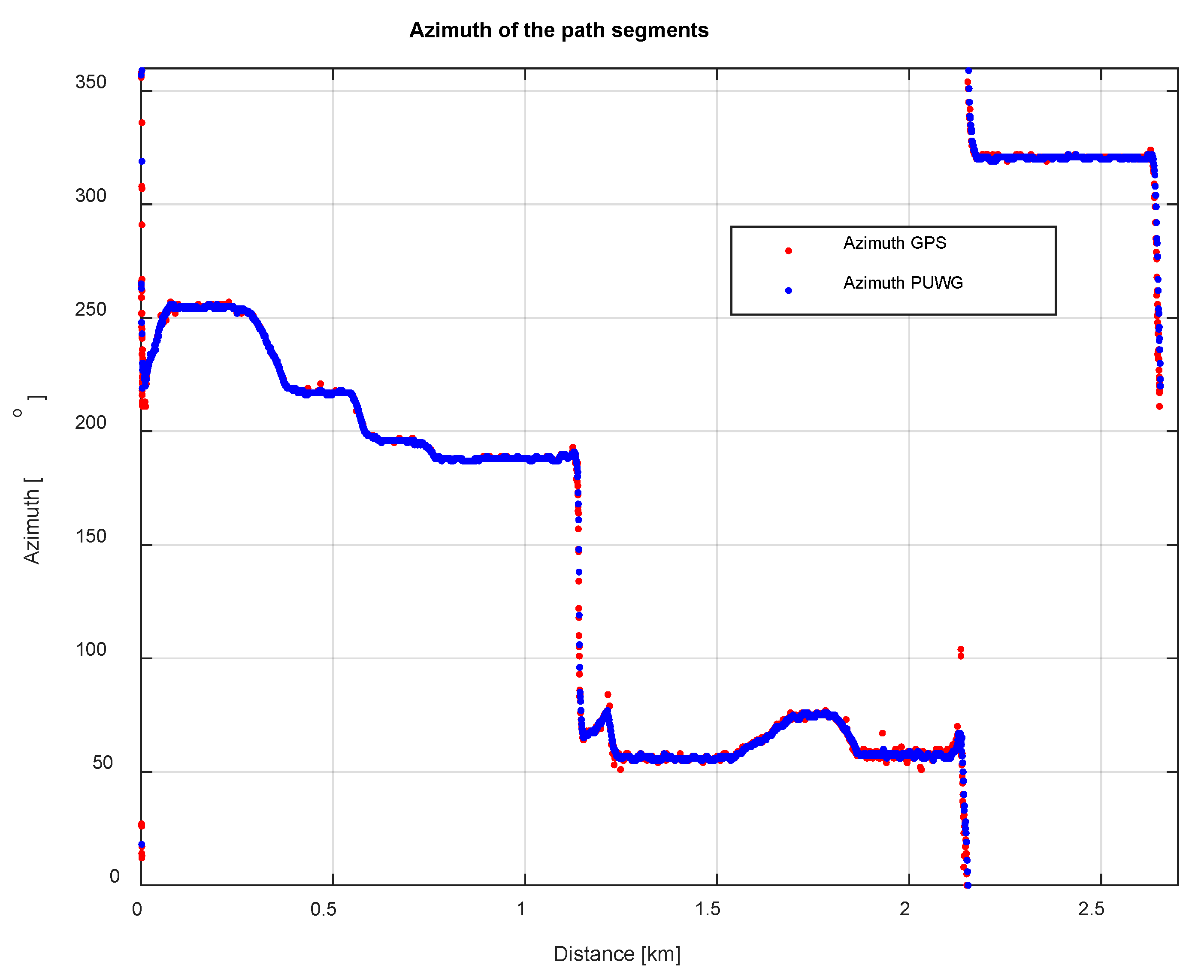
Wind speed and direction have an important impact on aerodynamic drag [23]. It is important to know about the azimuth that changes over time in the direction of movement. Figure 21 shows the results of calculating the azimuth of individual sections of the averaged path as a function of the distance traveled, which is obtained from GPS coordinates and from rectangular coordinates. In this case, there were also slight fluctuations in the function, which were eliminated using the usual operation of truncating the values to full angles.
4. Conclusions
From the user’s point of view, the bicycle computer is a “black box”, as the methods of processing the measurement signals are not precisely known and are not disclosed by the manufacturer. In this part of the article, only the quality of the recorded data from the GPS module and the barometric altimeter was assessed. However, these are very important data when trying to reconstruct the movement of the bicycle and energy demand.
The first conclusion that can be made is that the data logging frequency every one second is at the limit of the usefulness of the data for further processing. Much better results could be obtained if this frequency was at least 5 Hz, which is standard for a typical GPS module. Especially in the case of many low-cost devices such as a GPS tracking unit (GPS data logger), localizations are stored in the tracking unit or transmitted with a frequency of 5–10 Hz. A higher recording frequency would allow the use of our own methods of filtering GPS data and perhaps a more accurate mapping of the trajectory of the bicycle’s movement. The research was conducted on one model of a bicycle computer, but to the authors’ knowledge, competing bicycle computers have identical data recording parameters.
Dynamic Time Warping (DTW) and the hierarchical averaging method are very effective for determining the average trajectory. After transforming the averaged trajectory from GPS coordinates to rectangular coordinates of the map, further analyses can be performed, including the determination of a more precise route elevation based on geodetic data.
Altitude measurements with a barometric altimeter are quite precise given the nature of the changes. However, studies have shown that the bicycle computer has a problem calibrating the reference altitude. The slopes of the route determined by the bicycle computer are characterized by large fluctuations in values and generally with great noise effect. Therefore, these data seem of little use for studying the energy efficiency of bicycles. The proposed method of averaging the results from several runs allows obtaining more accurate slope characteristics of the route. However, if greater accuracy is needed, it is best to use geodetic data regarding the height of the terrain.
Thanks to the developed methods for averaging the route and additional information from the DTM, it was possible to quite precisely identify the parameters of the selected test route, which can be used in the energy balance models of bicycles.
In the tests carried out, all data available for the bicycle computer were recorded. Data related to speed, cadence, and power will be discussed in the next part of the article.
Author Contributions
Conceptualization, A.K., T.M. and Z.S.; methodology, A.K., T.M. and Z.S.; software, A.K., T.M. and Z.S.; validation, A.K., T.M. and Z.S.; formal analysis, A.K., T.M. and Z.S.; investigation, A.K., T.M. and Z.S.; resources, A.K., T.M. and Z.S.; data curation, A.K., T.M. and Z.S.; writing—original draft preparation, A.K., T.M. and Z.S.; writing—review and editing, A.K., T.M. and Z.S.; visualization, A.K., T.M. and Z.S.; supervision, A.K., T.M. and Z.S.; project administration, A.K., T.M. and Z.S.; funding acquisition, A.K., T.M. and Z.S. All authors have read and agreed to the published version of the manuscript.
Funding
This research received no external funding.
Institutional Review Board Statement
Not applicable.
Informed Consent Statement
Not applicable.
Data Availability Statement
The data presented in this study are available on request from the authors.
Conflicts of Interest
The author declares no conflict of interest.
References
- Charvátová, H.; Procházka, A.; Vyšata, O. Motion Assessment for Accelerometric and Heart Rate Cycling Data Analysis. Sensors 2020, 20, 1523. [Google Scholar] [CrossRef] [PubMed] [Green Version]
- Karetnikov, A.D. Application of Data-Driven Analytics on Sport Data from A Professional Bicycle Racing Team. Master’s Thesis, Eindhoven University of Technology, Eindhoven, The Netherlands, 2019. [Google Scholar]
- Chen, F.; Turoń, K.; Kłos, M.; Czech, P.; Pamuła, W.; Sierpiński, G. Fifth-generation bikesharing systems: Examples from Poland and China. Sci. J. Sil. Univ. Technol. Ser. Transp. 2018, 99, 05–13. [Google Scholar]
- Hurwitz, D.; Horne, D.; Jashami, H.; Abadi, M. Bicycling Simulator Calibration: Speed and Steering Latency; Pacific Northwest Transportation Consortium: Seattle, WA, USA, 2019; Volume 12, pp. 1–21. [Google Scholar]
- Favero Electronisc SLR. Influence of Angular Velocity of Pedaling on the Accuracy of the Measurement of Cyclist Power. Research article. Available online: https://cycling.favero.com/ (accessed on 18 January 2022).
- Desai, E.; Wang, P.; Suway, J.; Engleman, K. Bicycle GPS Positional Accuracy; SAE Technical Paper; SAE: Warrendale, PA, USA, 2021; Volume 1, pp. 1–7. [Google Scholar]
- Lißner, S.; Huber, S. Facing the needs for clean bicycle data—A bicycle-specific approach of GPS data processing. Eur. Transport. Res. Rev. 2021, 13, 1–14. [Google Scholar] [CrossRef]
- Welch, G.; Bishop, G. An Introduction to the Kalman. Filter. In Computer Graphics; Addison-Wesley: Boston, MA, USA; ACM Press: Los Angeles, CA, USA, 2001. [Google Scholar]
- Deep, A.; Mittal, M.; Mittal, V. Application of Kalman Filter in GPS Position Estimation. In Proceedings of the IEEE 8th Power India International Conference (Piicon), Jaipur, India, 13–15 December 2018. [Google Scholar]
- Gabaglio, V.; Ladetto, Q.; Merminod, B. Kalman Filter Approach for Augmented GPS Pedestrian Navigation; GNSS: Sevilla, Spain, 2001; pp. 1–5. [Google Scholar]
- Beato, M.; Bartolini, D.; Ghia, G.; Zamparo, P. Accuracy of a 10 Hz GPS Unit in Measuring Shuttle Velocity Performed at Different Speeds and Distances (5–20 M). J. Hum. Kinetics 2016, 54, 15–22. [Google Scholar] [CrossRef] [PubMed] [Green Version]
- Ranacher, P.; Brunauer, R.; van der Spek, S.; Reich, S. What is an Appropriate Temporal Sampling Rate to Record Floating Car Data with a GPS? ISPRS Int. J. Geo-Inf. 2016, 5, 1. [Google Scholar] [CrossRef] [Green Version]
- Jiménez-Meza, A.; Arámburo-Lizárraga, J.; de la Fuente, E. Framework for Estimating Travel Time, Di-stance, Speed, and Street Segment Level Of Service (LOS), based on GPS Data. Procedia Technol. 2013, 7, 61–70. [Google Scholar] [CrossRef] [Green Version]
- Vaughan, N.; Gabrys, B. Comparing and combining time series trajectories using Dynamic Time Warping. Procedia Comput. Sci. 2016, 96, 465–474. [Google Scholar] [CrossRef] [Green Version]
- Yang, J.; Mariescu-Istodor, R.; Fränti, P. Three Rapid Methods for Averaging GPS Segments. Appl. Sci. 2019, 9, 4899. [Google Scholar] [CrossRef] [Green Version]
- Marteau, P.-F. Estimating Road Segments Using Kernelized Averaging of GPS Trajectories. Appl. Sci. 2019, 9, 2736. [Google Scholar] [CrossRef] [Green Version]
- Karney, C. Algorithms for geodesics. J. Geod. 2013, 87, 43–55. [Google Scholar] [CrossRef] [Green Version]
- Moritz, H. Geodetic Reference System 1980. J. Geod. 2000, 74, 128–133. [Google Scholar] [CrossRef]
- Szymanski, Z.; Jankowski, S.; Szczyrek, J. Reconstruction of environment model by using radar vector field histograms. In Photonics Applications in Astronomy, Communications, Industry, and High-Energy Physics Experiments; International Society for Optics and Photonics: Bellingham, WA, USA, 2012; Volume 8454, pp. 1–8. [Google Scholar]
- Geoportal. Available online: https://mapy.geoportal.gov.pl (accessed on 5 December 2021).
- Zaliva, V.; Franchetti, F. Barometric and GPS altitude sensor fusion. In Proceedings of the IEEE International Conference on Acoustics, Speech and Signal Processing (ICASSP), Florence, Italy, 4–9 May 2014; pp. 7525–7529. [Google Scholar]
- Wahoo Product FAQ. Available online: https://eu.wahoofitness.com/ (accessed on 18 January 2022).
- Osman, I. Wind speed, wind yaw and the aerodynamic drag acting on a bicycle and rider. J. Sci. Cycl. 2015, 4, 42–50. [Google Scholar]
Figure 1.
The bikes used for the tests.

Figure 2.
Cycling computer used for testing.

Figure 3.
Test route (Google Maps).

Figure 4.
An example of determining the averaged track.
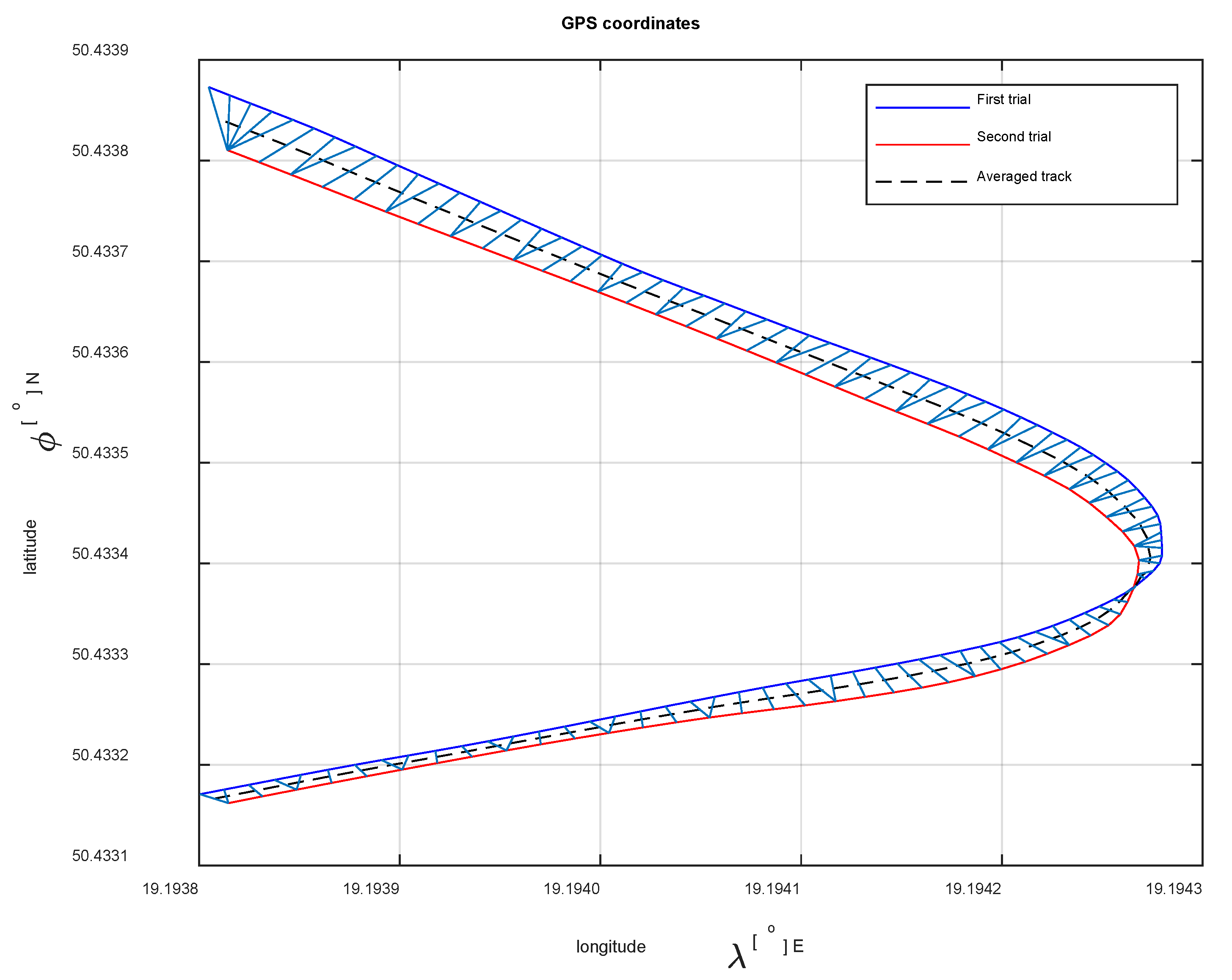
Figure 5.
Diagram of the hierarchical method of averaging multiple trajectories.
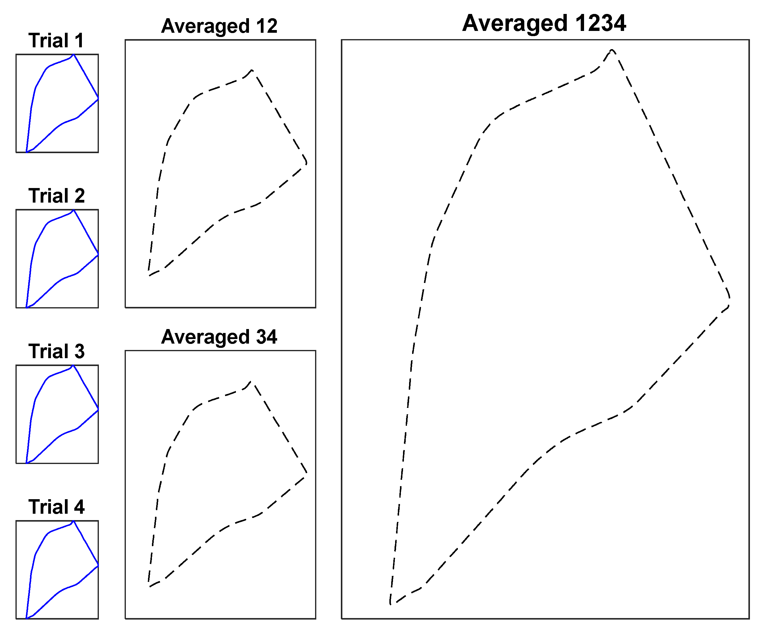
Figure 6.
Results of distance calculations with different methods compared.
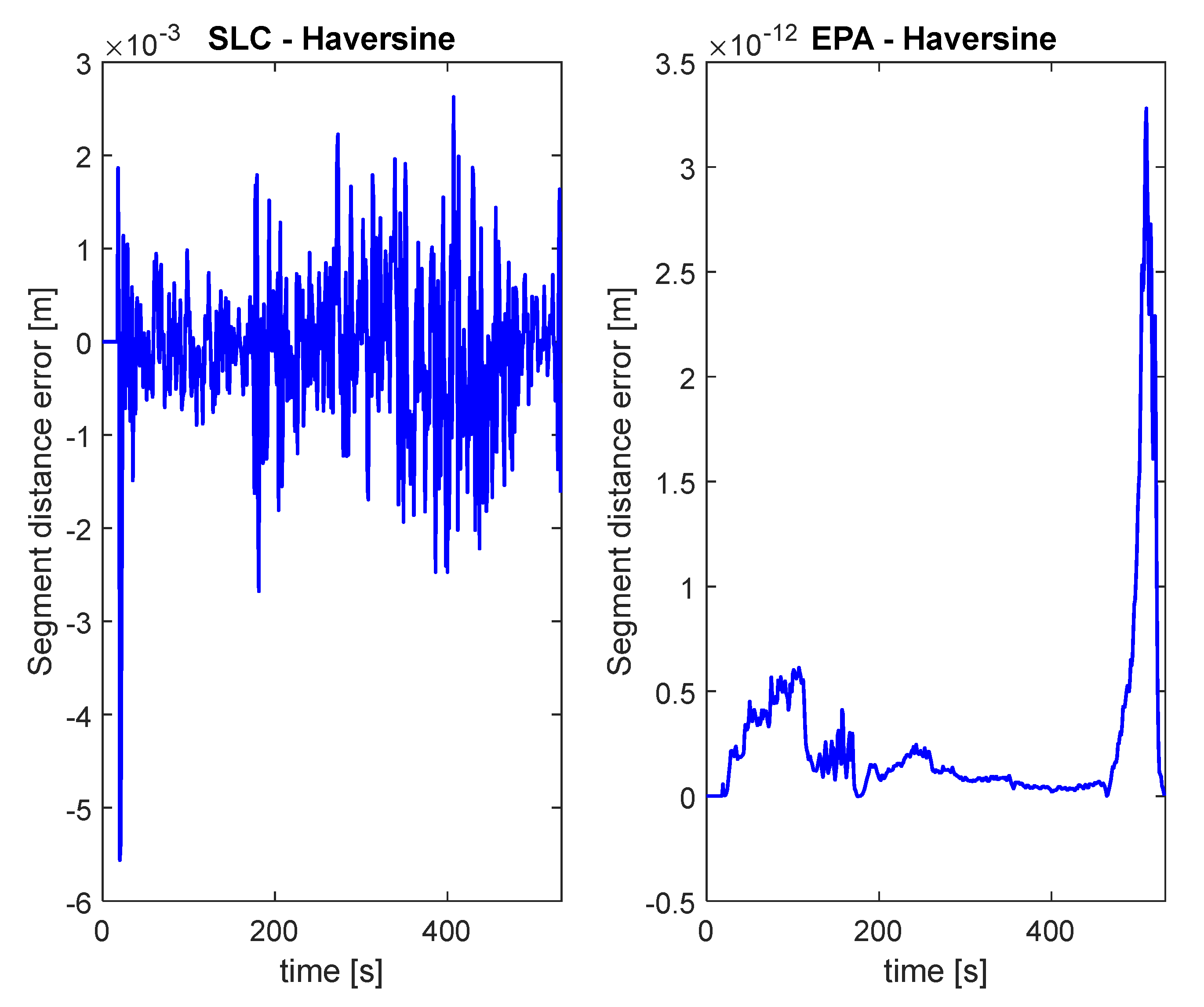
Figure 7.
An exemplary trajectory against the background of an orthophoto map.
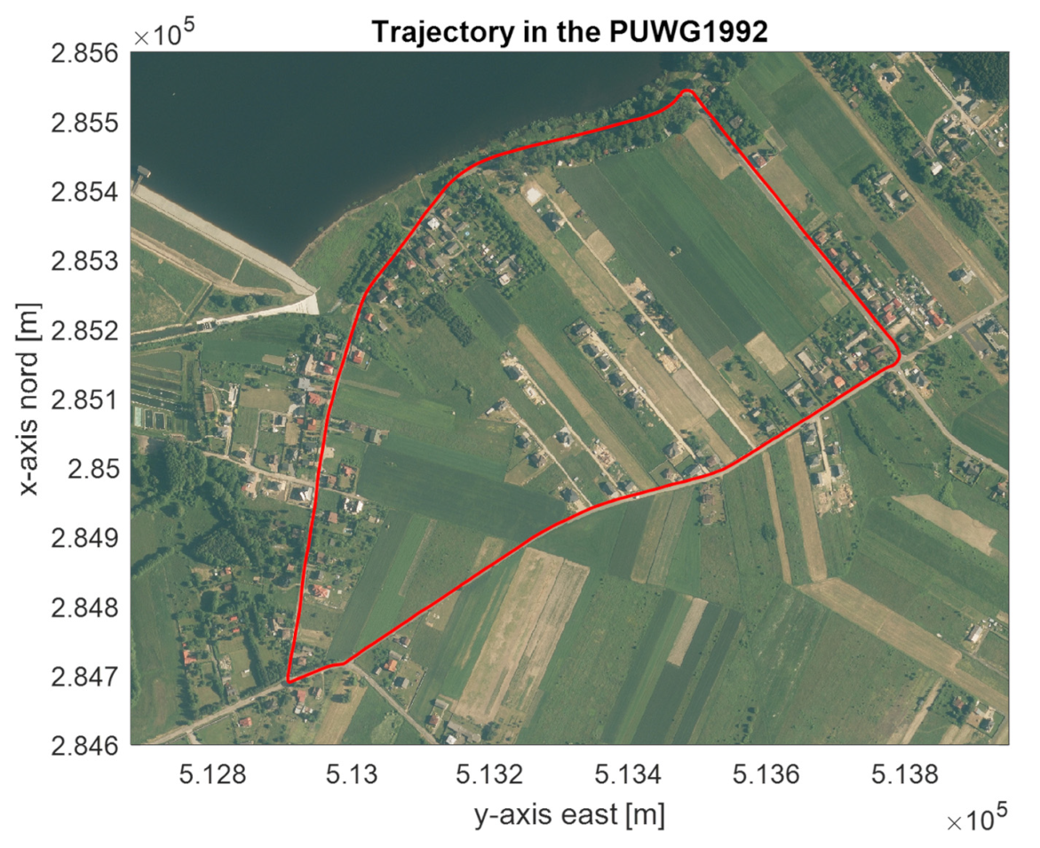
Figure 8.
DTM altitude map.

Figure 9.
Altitude raw and smoothed data (10 × 10 m section).

Figure 10.
Lagrange interpolation.
Figure 11.
Azimuth definition.
Figure 12.
Averaged trajectory from eight trials.
Figure 13.
Comparison of the trajectory length.
Figure 14.
Averaged path on the height map background.

Figure 15.
Comparison of registered altitudes and altitude determined from the DTM.

Figure 16.
The slope calculation results with different methods.

Figure 17.
Slope averaging using median filter.
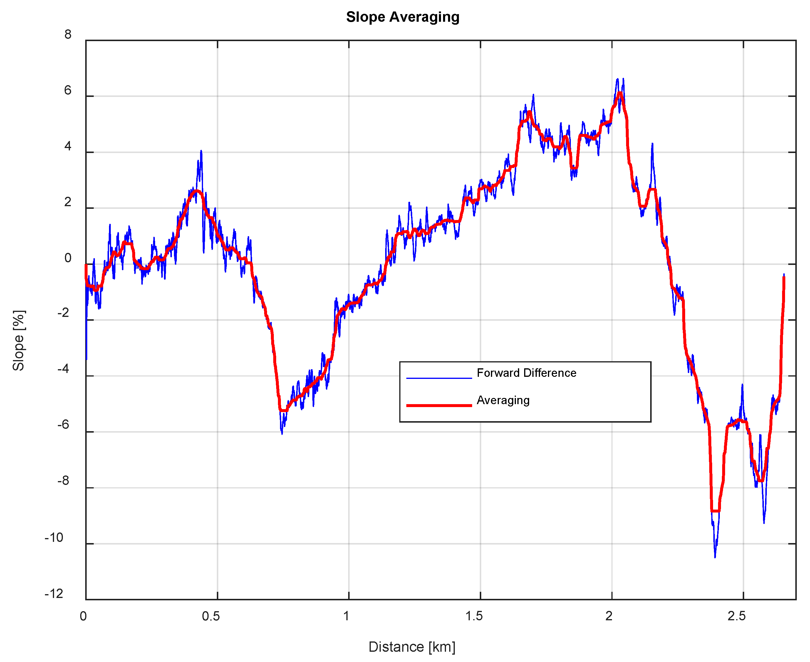
Figure 18.
Slopes recorded by the computer.

Figure 19.
(a) Calculated slopes based on height without smoothing. (b) Calculated slopes based on height without smoothing.
Figure 19.
(a) Calculated slopes based on height without smoothing. (b) Calculated slopes based on height without smoothing.
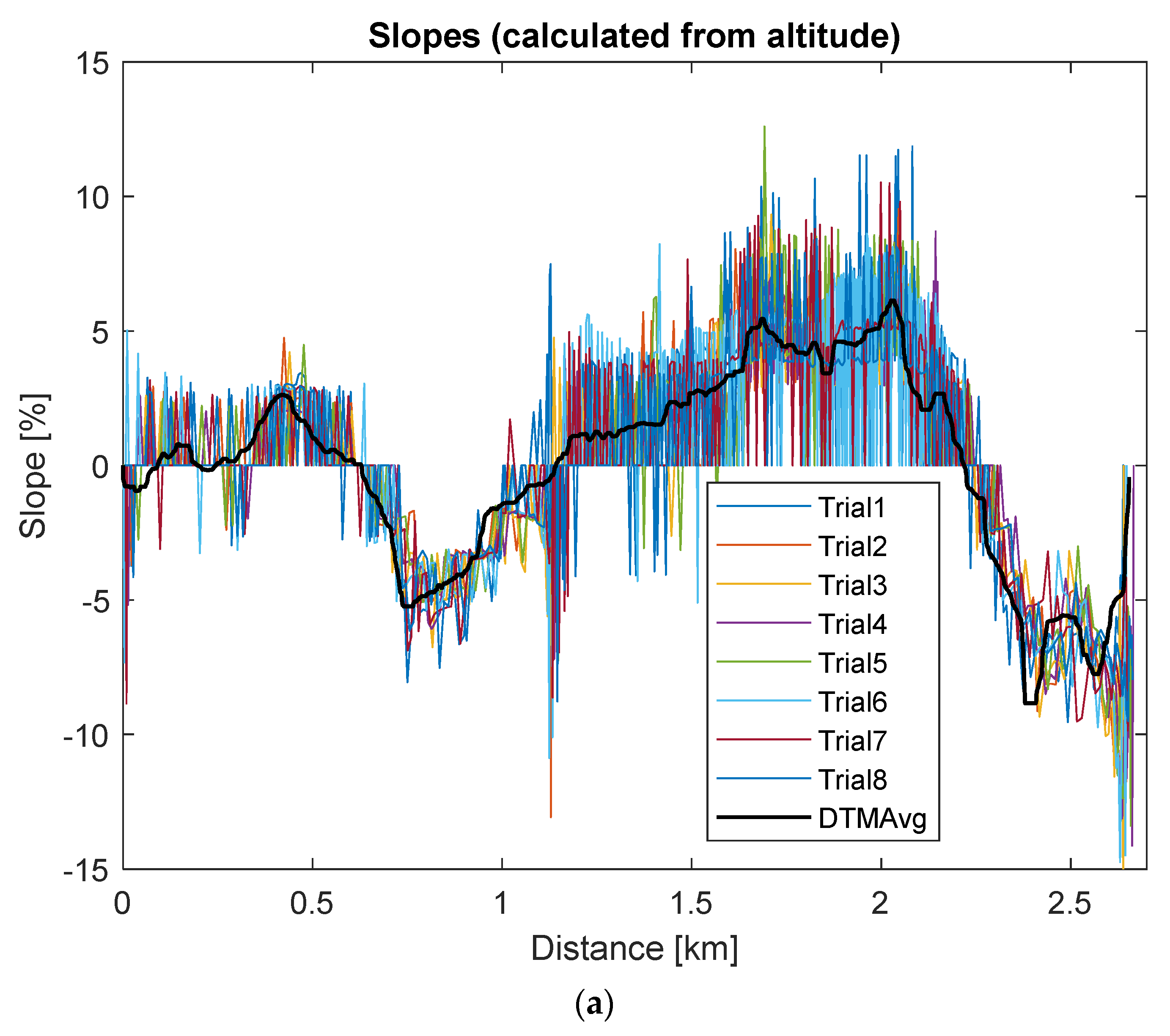
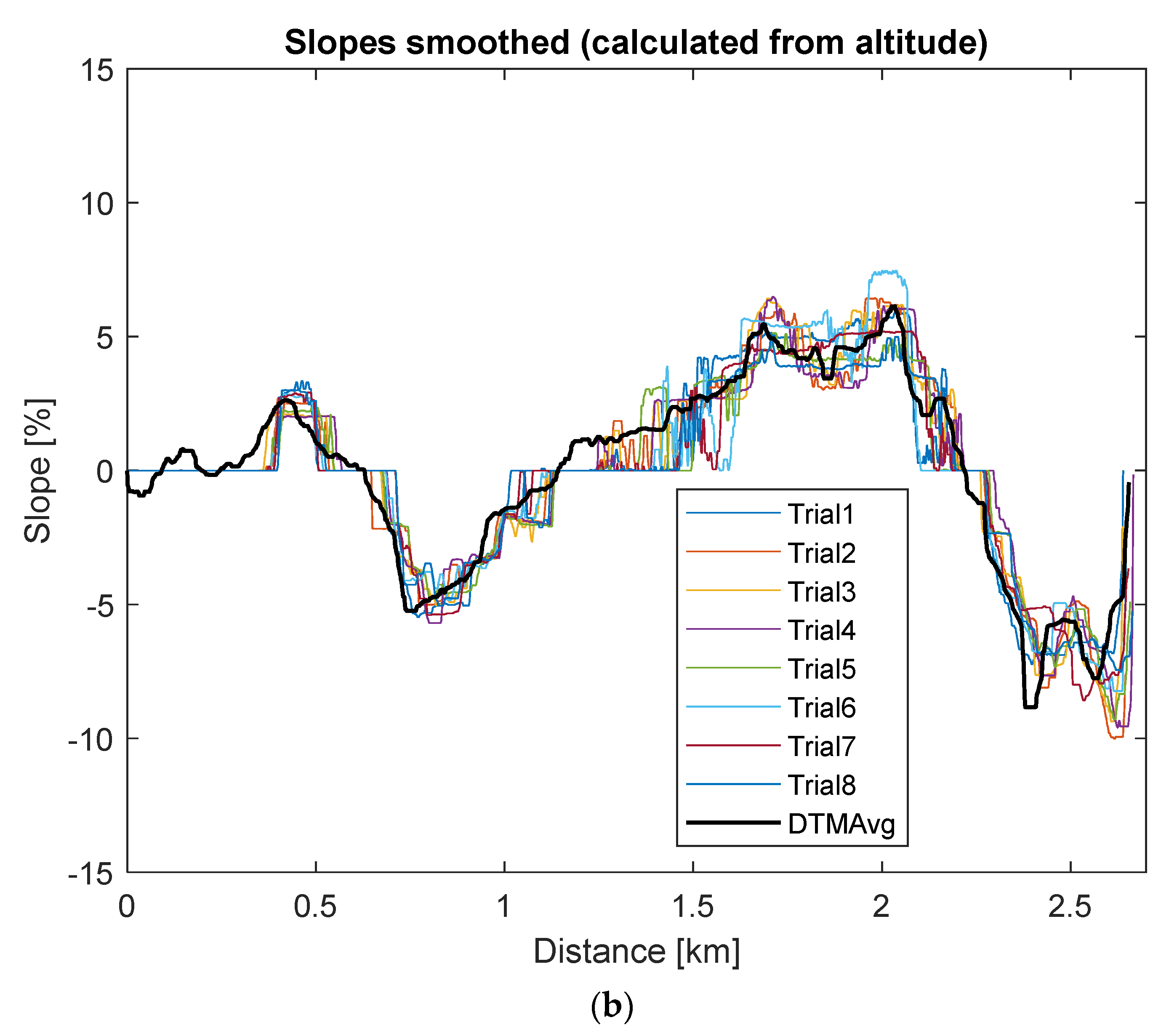
Figure 20.
Smoothed slopes from trials and from geodetic data.

Figure 21.
Azimuth calculations.

Table 1.
Selected trials.
| Trial | 1 | 2 | 3 | 4 | 5 | 6 | 7 | 8 |
|---|---|---|---|---|---|---|---|---|
| Time [s] | 469 | 353 | 342 | 344 | 394 | 532 | 440 | 398 |
Publisher’s Note: MDPI stays neutral with regard to jurisdictional claims in published maps and institutional affiliations. |
© 2022 by the authors. Licensee MDPI, Basel, Switzerland. This article is an open access article distributed under the terms and conditions of the Creative Commons Attribution (CC BY) license (https://creativecommons.org/licenses/by/4.0/).
Share and Cite
MDPI and ACS Style
Matyja, T.; Kubik, A.; Stanik, Z. Possibility to Use Professional Bicycle Computers for the Scientific Evaluation of Electric Bikes: Trajectory, Distance, and Slope Data. Energies 2022, 15, 758. https://doi.org/10.3390/en15030758
AMA Style
Matyja T, Kubik A, Stanik Z. Possibility to Use Professional Bicycle Computers for the Scientific Evaluation of Electric Bikes: Trajectory, Distance, and Slope Data. Energies. 2022; 15(3):758. https://doi.org/10.3390/en15030758
Chicago/Turabian StyleMatyja, Tomasz, Andrzej Kubik, and Zbigniew Stanik. 2022. "Possibility to Use Professional Bicycle Computers for the Scientific Evaluation of Electric Bikes: Trajectory, Distance, and Slope Data" Energies 15, no. 3: 758. https://doi.org/10.3390/en15030758
Note that from the first issue of 2016, this journal uses article numbers instead of page numbers. See further details here.