
Realistic Load Modeling for Efficient Consumption Management Using Real-Time Simulation and Power Hardware-in-the-Loop


GECAD—Research Group on Intelligent Engineering and Computing for Advanced Innovation and Development, LASI—Intelligent Systems Associate Laboratory, Polytechnic of Porto, 4200-072 Porto, Portugal
*
Author to whom correspondence should be addressed.
Energies 2023, 16(1), 338; https://doi.org/10.3390/en16010338
Submission received: 28 September 2022
/
Revised: 7 December 2022
/
Accepted: 20 December 2022
/
Published: 28 December 2022
(This article belongs to the Special Issue Smart Energy Systems: Control and Optimization)
Abstract
:By empowering consumers and enabling them as active players in the power and energy sector, demand flexibility requires more precise and sophisticated load modeling. In this paper, a laboratory testbed was designed and implemented for surveying the behavior of laboratory loads in different network conditions by using real-time simulation. Power hardware-in-the-loop was used to validate the load models by testing various technical network conditions. Then, in the emulation phase, the real-time simulator controlled a power amplifier and different laboratory equipment to provide a realistic testbed for validating the load models under different voltage and frequency conditions. In the case study, the power amplifier was utilized to supply a resistive load to emulate several consumer load modeling. Through the obtained results, the errors for each load level and the set of all load levels were calculated and compared. Furthermore, a fixed consumption level was considered. The frequency was changed to survey the behavior of the load during the grid’s instabilities. In the end, a set of mathematical equations were proposed to calculate power consumption with respect to the actual voltage and frequency variations.
1. Introduction
1.1. Context and Motivation
The increasing use of Distributed Energy Resources (DERs) in electricity networks is moving to a decentralized power system [1]. Smart grids are electrical power infrastructures that make intelligent decisions about the conditions of the electrical power system to maintain the stability of the network [2]. In fact, smart grid technologies open up new opportunities for consumers to actively participate in power system operation through Demand Response (DR) programs [3]. In a cooperative way, consumers can be part of energy communities to improve their benefits resulting from flexibility through DR programs [4,5]. Energy storage means are another way for the flexible management of energy resources enabled by the smart grid [6]. Moreover, aggregators enable small- and medium-scale consumers and producers to actively participate in the power system and contribute to electricity markets [7].
DR is a series of activities that respond to peak demand or electricity prices by regulating or restricting the operation of consumer equipment, resulting in benefits for all parties involved [8]. Further advancements in DR and the massive implementation of DR programs require extensive research, namely regarding load modeling. Laboratory emulation and experimental validation play a key role in the realistic testing and validation of the theoretical hypothesis [9] and are crucial if DR schemes rollout are to be envisaged. Simulation methods and infrastructures are a must-have for any business model before mass production, as they avoid possible financial losses and ensure the safety of the system [10]. In this context, real-time simulation and hardware-in-the-loop are good means by which to validate the envisaged business models, as they integrate and compare the results of real and simulated environments [11].
The motivation of the authors of the present paper is to find a way to accurately model actual load consumption in the presence of a range of voltage and frequency deviations. This is important in the context of energy resource management; namely in DR programs. One should know the consumption of the same load/device at different points of the network. Accordingly, this paper aims to design and implement a laboratory testbed by which to examine the behavior of consumers facing fluctuations in voltage and frequency. To do so, a set of laboratory loads emulates actual consumers that are associated with an aggregator. The testbed proposed in this paper (Figure 1) is part of a decision support platform, which considers different perspectives and players, ranging from Distribution System Operators (DSOs) and aggregators to single consumers to improve the efficiency of the entire power system, while ensuring that individual players’ goals and interests are considered.
1.2. Related Literature
There have been several similar works reported in the literature that focus on this topic. In [12], the authors proposed a flexible and embedded real-time simulator platform to provide optimized power flow solutions. Their simulation results demonstrated the accuracy and timeliness of the proposed real-time simulation based on the IEEE 37 bus test feeder emulation. The authors in [13] used PHIL-based test setups to study the microgrid dynamics. They demonstrated the use of a commercial high-bandwidth voltage amplifier as a dynamic three-phase power converter emulator. In [14], the authors reported the implementation of a real-time simulation platform for a curtailment service provider as an aggregator entity connected to a larger distribution network. The platform was able to integrate optimization methods for energy resource scheduling and efficient operation of the aggregator. In the work described in [15], the authors used a real-time simulation model to technically validate the implementation of the ramp period and the requested demand reduction during a DR event. In [16], the authors compared two different setups for the evaluation of components and systems focused on undisturbed operational conditions. The first setup was a conventional PHIL setup and the second was a simplified setup based on a quasi-dynamic PHIL approach, which involves fast and continuously steady-state load flow calculations. With a focus on distribution networks with a high penetration of renewable energy sources, the work in [17] used real-time digital simulation and hardware-in-the-loop methods for the validation of prototype controllers. The work in [18] used PHIL to validate a voltage regulation scheme for distribution networks with renewables. The amplifier controls the voltage applied, as decided by the voltage regulation model. Focusing on distribution grid stability, in [19], an innovative bench focusing on dynamic behavior simulation was presented. An extensive study was provided on the inaccuracies between the real devices and the virtual model. The review in [20] summarized the state-of-the-art in real-time simulation and hardware-in-the-loop models related to one of the major simulator manufacturers. The focus was on power electronics modeling and testing.
From the perspective of load modeling, in [21], synthetic electricity load profiles were generated. Such profiles were obtained by deterministic and stochastic methods. In [22], profiles were generated for EV charging in buildings with a various number of chargers. The potential impact of DR was evaluated by comparing charging profiles and adjusting the maximum power of chargers. PHIL or real-time simulation features were not used in these studies, despite them focusing on load modeling.
1.3. Contribution
Using PHIL is necessary in order to dynamically control the voltage and frequency of the source to the load under study using software. While an amplifier changes the source characteristics, the real-time simulation target provides accurate variations in the source characteristics as desired. A campaign of different voltage and frequency variations being manually made would take time and potentiate systematic errors.
Therefore, the objective of the present work is to automatically run a set of source conditions and obtain accurate parameters for the load models in Simulink, while other works in the literature have focused on the control approaches for voltage and frequency stability, with load study being disregarded. This is the reason why the present work is so important compared to the aforementioned instances in the literature.
Taking into account the current state-of-the-art and previous advancements, the main contributions of this paper are centered on:
- Developing an innovative approach to model the consumption of electrical loads in the function of frequency and voltage variations;
- Implementing a testbed by which to survey the behavior of consumers facing source parameter variation; namely, voltage drop;
- Comparing the theoretical and experimental behaviors of laboratory load models under actual conditions;
- Obtaining accurate parameters for the MATLAB™/Simulink (Matlab version 7.13 (R2011b), Simulink version 7.8 (R2011b)) load model, according to the real loads in a laboratory;
- Controlling the PHIL device from OP5600 and collecting the results from the loop, in real time;
- Providing a set of equations to model the active power consumption of a load in the function of the source voltage and frequency. For a specific load, and a given frequency, the active power is obtained with the input of voltage. Regression tools are used to obtain such equations.
The innovative scientific contribution of this paper is given to the application of PHIL and real-time simulations to propose a load model using a set of laboratory devices. A simplified equation set, obtained with linear regression, is provided as the input parameters to the Simulink load models. Although there is a considerable number of research works in the literature focused on real-time simulation concepts, the use of PHIL and real-time simulation for estimating the behind-the-meter load profiles represents a gap in the literature. Therefore, this lack of research has encouraged the authors to focus on such topics.
The rest of the paper is organized as follows: After this introductory section, a detailed explanation of the developed methodology is described in Section 2. Section 3 describes a case study to illustrate the test and validation of the system’s performance; there are some instabilities in the network. The case study results are presented in Section 4, regarding data analysis and other interesting results. Finally, in Section 5, the main conclusions of the work are described.
2. Developed Methodology
This section presents the developed method for simulation and emulation.
2.1. Architecture
The model presented in this paper is part of a decision support platform for DR programs. Figure 1 illustrates the architecture of the decision support platform. This platform considers different perspectives and players, ranging from DSOs and aggregators to single consumers. This proposed platform provides the tools required for several decision-making approaches regarding DR. The following proposed features apply:
- Implement DR and aggregator aspects using a diversity of load models and existing resources. This platform integrates network simulation models to analyze the consumers’ behavior in the implementation of DR. Moreover, it can control various actual appliances through various communication protocols, such as Ethernet (MODBUS TCP/IP);
- Combination of the OP5600 and PHIL devices provide an integration of real and simulation environments. Therefore, actual results adapted from real resources are used in a simulation environment (i.e., MATLAB™/Simulink) in real time;
- Various actual case studies implementation: where resource aggregation and scheduling, distributed control approaches, and real-time simulation are the main features;
- Capability of information exchange between different network nodes in real time. For example, while the aggregator intends to apply a DR event, it should be aware of real-time consumption;
- Receiving a notification from the aggregator regarding a DR event, and managing the related appliances based on the user preferences;
- Technical and practical features of DR are verified, and the use of adequate approaches to address the potential of customers for the DR program becomes feasible;
- Estimation of the amount of consumption of a specific device for the DR events.
This paper’s focus is given to load modeling, as seen in the top-right corner of Figure 1. This feature is more applicable in DR programs, such as DLC, where the aggregator requires the real-time consumption of a specific load. The developed load modeling is based on a set of experimental and laboratory tests for studying the behavior of a load using the real-time simulator (OP5600) and a power amplifier. Its use in this model emulates a local power supply separate from the utility grid, in order to modify the electricity supply parameters (i.e., voltage, frequency, and phase angle) and survey the reaction of the electricity consumer or producer. The outputs of the OP5600 are set to the voltage and frequency that the power amplifier needs to emulate.
Therefore, through the load modelling approach proposed in this paper, the aggregator can calculate a specific load consumption, applying the following steps:
- defining the power parameters in the real-time simulator’s network model. The effective parameters in this context include voltage amplitude, phase angle, and frequency;
- the network parameters are set, and the real-time simulator specifies the consumption for the loads. The defined rates in this level are dependent on the capabilities of the consumer devices;
- through the combination of consumption levels and electricity supply parameters, several tests are performed;
- when all data and results have been gained from the model, it is necessary to synchronize the amplifier and measurement data, as these may have some duplicate data in the gained outcomes;
- the acquired information must be analyzed to validate the model’s performance;
- mathematical equations to be used as a load model are obtained. These mathematical equations show the relation between the voltage variation and the power consumption of the load;
- The accuracy and errors of the model are computed. The average, maximum, and minimum errors are analyzed for a specific range of data.
Figure 2 illustrates the required phases for studying the load behavior. It starts with the definition of the parameter’s variation range, followed by the identification of the loads consumption (as seen on right side of Figure 2, several loads can be considered). In the third step, all of the tests and measurements are conducted. After data processing, which includes the removal of duplicates and the synchronization of data, the load model is obtained.
2.2. Implemented Laboratory Setup
The OP5600 is a powerful machine for rapid control prototyping through the HIL approach. In fact, the OP5600 is based on MATLAB™/Simulink, which is accommodated by the main software of the OP5600 (RT-LAB). The OP5600 controls HIL devices by several digital and analog I/O slots, which receive controlling commands from the Simulink model. More information regarding the performance of the OP5600 is available in [15,23]. The laboratory setup and configurations of the developed model are presented in Figure 3.
The second component of the system is a three-phase power amplifier with a rated power of 3 kW (PA-3 × 1000—www.puissanceplus.com, accessed on 10 September 2022). To control this amplifier, OP5600 converts the associated power parameters to a range between 0 V to 10 V and sends it to the amplifier through an analog output slot. In other words, the amplifier receives 0 V to 10 V Direct Current (DC) as inputs. It gives an output of 0 V to 250 V Alternating Current (AC) according to the pre-defined setting configuration.
As Figure 3 shows, the amplifier’s output power is connected to a laboratory resistive load with a nominal capacity of 8 kW. It is equipped with several relays and automatic switches connected to the digital output slot of the OP5600.
The time interval in the real-time simulation between the acquired data plays a key role. Whenever the time interval between the data is closer and near to zero, the model will have more accurate results, in near to real time. This is limited by the characteristics and capacities of the system’s computational infrastructures.
As shown in Figure 3, there are three time windows for data transmission between all infrastructure and devices. The first time window is when the OP5600 sends and receives data to/from the amplifier for configuring the power parameters. In the second time window, the OP5600 transmits a reference consumption to the related resistive load. Finally, in the last time window, the energy meter conveys the real-time information to the OP5600. Furthermore, the time interval between the acquired data is different in each time window according to the devices’ capabilities. The time interval for data transmission between the OP5600, the power amplifier, and the resistive load is set to 50 µs (as shown in Figure 3). In this specific model, 50 µs time intervals are small enough for the OP5600 to process the data and provide acceptable outcomes. The energy meter measures active power, voltage, current, and frequency with 1 s intervals.
In summary, in order to obtain the results presented in this paper, it is necessary to:
3. Case Study
The case study employs the laboratory devices presented in Section 2.1 to implement different realistic scenarios. In this case study, the OP5600 is configured to control the amplifier concerning the power parameters adapted from the network simulation. Furthermore, it manages the consumption of the resistive load according to the simulation requirements.
The case study’s focus is given to varying the voltage and frequency of each phase, as shown in Table 1. The voltage amplitude is changed from 184 V to 250 V with a step size of 2.6% of the setpoint value (around 6 V in each step size).
In fact, 184 V are five steps below the setpoint value, and 250 V is five steps over the setpoint. In this way, it is possible to have 11 different and separate voltages in each phase. The same approach is followed for the frequency, where five different possibilities are been used; from 49 Hz to 51 Hz with a step size of 1% of the setpoint value (50 Hz). The phase angle is kept unchanged during the case study. In the first phase, it is considered to be zero, and, in the second and third phase, it is set to 2π/3 and −2π/3, respectively.
Therefore, by combining all of these possibilities, a total number of 6655 scenarios are created and implemented in this case study. Among these 6655 scenarios, 3355 of them have been obtained to restrict the sum of the amplitudes, so that all three phases should be less than or equal to 690 V, which is the maximum value allowed by the amplifier to supply an external load. According to the amplifier’s technical limitations, it is not possible to supply the 8 kW resistive load in its full capacity. Therefore, five various load steps are considered in this case study. The considered load steps are: 0.40 kW, 0.85 kW, 1.30 kW, 1.70 kW, and 2.20 kW. These values have been selected according to the technical features of the resistive loads.
All of the parameters demonstrated in Table 1 are performed for each single load step. Additionally, as the system works in real time, a reference signal, including consumption, amplitude, frequency, and phase angle, is automatically transmitted ever 5 s from the OP5600 to the amplifier and resistive load. Then, the energy meter transmits back the real-time information to the OP5600 in 1 s time intervals. The amplifier can receive these values from other data providers, such as a wave generator.
This case study’s procedure is automatically configured by the OP5600, and it autonomously operates and executes all scenarios. For each load level, a huge amount of data regarding voltage, current, and active power are measured by the energy meter. Some parameters remained unchanged for 5 s during the emulation, and only afterward are new values sent. Therefore, it is necessary to perform data cleaning at the end of the emulation, where the repeated values are eliminated.
4. Results
This section presents the acquired results from the case study.
4.1. Single Step Results
A single scenario has been selected to highlight the data related to each scenario. In the selected scenario, the load is 2.2 kW and the voltage in the three-phases vary from 184 V to 260 V. In this test, the voltage of phase 1 is set at 184 V; phase 2 is set at 230 V; and phase three is set at 260 V. The frequency in all three phases is constant and set to 50 Hz. Figure 4 shows the first 3 s of the reference voltage signal for the amplifier. It would be interesting to have the behavior signals of the transistors in the amplifier. However, using this equipment, one must provide sine wave signals, which are then automatically converted to the respective signals of the transistors.
As Figure 4 illustrates, in the first moments of emulation, the sinuous wave of the voltage in each phase is trying to reach the desire frequency level (i.e., 50 Hz). This is due to the frequency ramp that has been configured in the Simulink model. After a while, all signals have reached 50 Hz.
Figure 5 illustrates the output results for 0.1 s (2000 periods of 50 µs). Figure 5 shows that the amplifier’s voltage has reached the desired level. Furthermore, phase 1 has a lower voltage compared to the other phases. Therefore, the resistive load is supplied with a lower active power in phase 1, as the current cannot reach the nominal value. On the other hand, phase 3, with a higher voltage, compensates for the voltage drop of phase 1. The amplifier’s technical limitations do not allow it to go further than 250 V. Therefore, as shown in Figure 5A, the peak of the sinuous wave in phase 3 is cut and limited to 250 V.
It can be concluded that the consumption of the load is lower than the desired level (i.e., 2.2 kW in this test). On the other hand, it is possible to calculate the delivered power from the amplifier to the resistive load.
4.2. Data Measurements and Cleaning
First, the data have to be organized in order to analyze them, as the obtained results may vary from the real results. Table 2 shows the information related to the quantity of acquired data during the emulations. The parameter settings transmitted from the OP5600 to the power amplifier have been automatically changed every 5 s, and the energy meter transmits the information every 1 s. This means that, every 5 s, the information for each parameter is obtained five times. The amount of expected data registered in Table 2 is calculated by multiplying the number of scenarios with A1 + A2 + A3 ≤ 690 V, from Table 1, by five times. Therefore, the expected amount of data for the case study is 16,775.
In Table 2, obtained data are the actual data recorded from the energy meter, and the data after cleaning are sifted information without the repeated values. There is a difference between the expected data and the actual obtained values. This is due to device failures and package loss in communication lines during the emulations. In fact, these differences are one of the key features of real-time simulations and laboratory validations. The need for technical verifications and emulation tools, as well as prototyping, is always essential for avoiding failures in any model’s future and implementation level. Therefore, all of the results shown in this paper are based on the actual obtained data after the cleaning process.
4.3. Data Analysis and Load Modeling
After measuring and cleaning the data, linear regression is applied. As the measured data includes the source voltage and frequency and the output active power, a linear equation is obtained to represent the changes in the active power as a function of the source voltage and frequency. Table 3 summarizes the linear relations between the total power consumption of the load (PSUM) and total voltage (VSUM) for various levels of frequency and load consumption rates.
As is clear in Table 3, there are two regression approaches for each load level. In regression approach (A), there is one regression equation for each frequency level in the specified load level. However, in regression approach (B), there is only one regression equation for all frequency levels. In other words, the regressions in approach (A) are calculated based on the data in each specific frequency; the regressions in approach (B) are calculated with respect to all frequency levels. Therefore, using the equations shown in Table 3 shows that it is possible to forecast the load’s real-time consumption using total real-time voltage and frequency.
To make the results of Table 3 clearer, suppose that an aggregator can control and manage a common device (e.g., a fan heater or water heater) of a customers in different geographical locations of the network. The information shown in Table 3 is for the device that the aggregator has information on. Furthermore, all customers are equipped with a smart meter, which means the network operator is aware of each customer’s total consumption, voltage, and frequency. However, the aggregator is not aware of the real-time consumption of each specific device. Therefore, it can anticipate the device’s consumption according to the regressions shown in Table 3, using the common voltage and frequency level.
In Table 3, PSUM varies depending on VSUM and the frequency for each load level. The PSUM has been obtained by reading the power consumption in the energy meter during the case study. VSUM has been calculated by adding the voltage of three phases measured by the same energy meter.
Regression approach (B), as shown in Figure 6, is based on the trendline of all frequency levels. All of the results shown in Table 3 are for a specific resistive load (shown in Figure 3). The results for other devices are different according to their technical features and practical characteristics. Moreover, charts A to E in Figure 6 represent the total power consumption results with 2,20 kW, 1.70 kW, 1.30 kW, 0.85 kW, and 0–40 W load levels, respectively. Furthermore, in each chart of Figure 6, a trendline equation has been calculated for the power consumption, so that it is possible to calculate the consumption for any desired voltage.
As Figure 6 illustrates, the power consumption for every frequency and voltage evolves in the same way. While the total voltage increases, the total power consumption also increases. However, there are values where the power consumption is not the same, which could be due to some simulation disparities. In charts B, C, and E of Figure 6, the values are more dispersed, unlike the charts A and D, in which the values are closer together.
As mentioned in Section 3, there is a limitation of voltage (up to 690 V) in the amplifier, which is the maximum allowable range for the amplifier to supply the loads.
Through these linear regression equations, the average, maximum, and minimum errors have been obtained for each load level’s linear power regressions and the linear power regression with the set of all load levels.
The regression calculation results in the trendline equation presented in Figure 6, where a linear regression is applied. For a more detailed analysis of the obtained regressions, regression parameters are listed in Table 4. Furthermore, error analysis is outlined in Figure 7 and Figure 8. This study is very important to verify the validity of the proposed simulation and emulation model.
The slope (“m”) can be positive, negative, or zero, and is obtained as shown in (1). The intercept (“c”) measures the length where the line cuts the y-axis from the origin, as represented in (2). The coefficient of determination (“r2”) is the proportion of variation in the dependent variable that is predictable from the independent variable(s), as in (3). In these equations:
y is the mean of the observed data;
yi is any value of the observed data;
y1 is the correspondence to x1;
y2 is the correspondence to x2;
fi is any fitted value.
Looking at the slope parameter (m), one can see that the active power has stronger dependence on the voltage for higher rated consumption (2.2 kW). The c parameter is in line with m. Moreover, regarding r2, one can see that it has no monotony with the variation in rated consumption. The higher r2 is for the highest rated consumption (2.2 kW), while the lower r2 is for the average rated consumption (1.3 kW). This means the variability in the consumption is explained by the variability in the voltage, with more strength relation for 2.2 kW and weaker relation for 1.3 kW.
Regarding the reliability of these results, it is important to mention that there is no human error interfering with the measurements, readings, and calculations, as the process is completely automated. In this way, if the process is repeated, it would be expected to obtain the same results; therefore, the results are reliable.
Figure 7 shows the error comparisons between each load level’s regression and the regression of all load levels, while the frequency is considered a fixed parameter in each step. The errors shown in this section are a comparison between the actual power consumption obtained from the energy meter during the case study and the calculated power consumption using the regression in each load and frequency level. In Figure 7A, the calculated average errors are compared, and it illustrates that the average error for each load level is approximately equal to zero. Furthermore, the average error calculated for the regression of all load levels is mostly higher than the calculated error for each load level’s singular regression. The same approach is also followed in Figure 7B to show and compare the maximum and minimum calculation errors. Figure 7B indicates that for both singular load level regression and all load level regression, maximum and minimum errors are almost identical.
In this context, it is interesting also to calculate the error using frequency variation. The same procedure shown in Figure 7 has been followed. However, in this part, frequency is varied from 49 to 51 Hz considering a fixed load level.
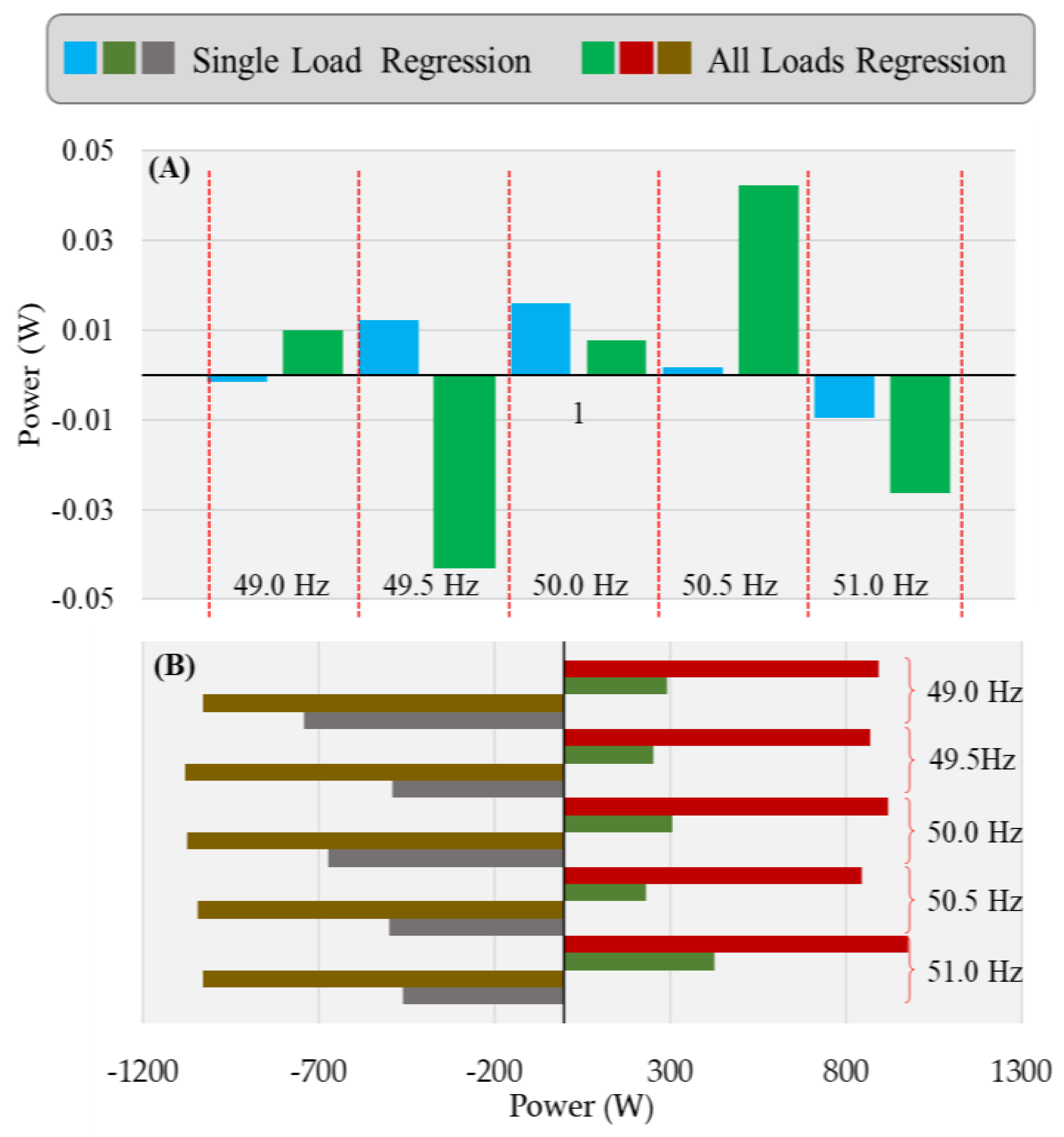
Figure 8 shows the error computations using frequency levels that compares outcome errors of the linear power regression equations for each frequency level and the linear power regression with the set of all frequency levels. In each frequency step shown in Figure 8, a fixed load level has been considered.
As is obvious in Figure 8A, the average error of singular frequency in 49.0 Hz is less than for other approaches. However, in Figure 8B, all frequency level regression’s maximum and minimum error are always greater than the regression of each singular frequency level. This is the most crucial point that can be concluded from the error results. The user must indicate which kinds of errors are more important for the model. If the average accuracy is the most important parameter, singular frequency regression at 49.0 Hz (Figure 8A) can be selected. However, if the maximum and minimum errors are vital for the model, other regression equations should be selected.
5. Conclusions
The main purpose of this study was to produce load modeling based on the laboratory experiments’ experimental data. A vast number of scenarios and possibilities were required to produce reliable results. In the first stage of the study, the related power parameters, namely voltage amplitude, the phase angle, and frequency, were defined in the real-time simulator. Then, they were transmitted to the three-phase power amplifier. The output power of the amplifier was connected to a laboratory resistive load, and its real-time power consumption was measured through an energy meter transmitted to the real-time simulator. After all data and results were gained from the model, data cleaning and organization were performed. The last and most crucial step was to analyze and validate the acquired information for producing mathematical equations.
In the case study, the voltage amplitude was changed from 184 V to 250 V with a step size of 2.6% of the setpoint value, obtaining 11 different values. The frequency created five values, between 49 Hz and 51 Hz, with step sizes of 1% of the setpoint value. The values of the phase angle were fixed, and the angle of the first phase was set on zero, the angle of the second and third phase was set on 2π/3 and −2π/3, respectively. Through a combination of all of these possibilities, and with some restrictions, 3355 scenarios were obtained. Due to the amplifier’s technical limitations, five load steps for the resistive load were considered: 0.40 kW, 0.85 kW, 1.30 kW, 1.70 kW, and 2.20 kW. For each single load step, a period of 68 min was considered for each possibility of the study, where the parameter variations were being carried out.
Through the obtained and cleaned results, two regression approaches were performed. The first was with one regression equation for each frequency level in the specified load level. Then, in the second approach, only one regression equation for all frequency levels was performed. A set of mathematical equations were proposed through the model results by which to calculate power consumption concerning the actual voltage and frequency variations. These equations are more applicable to calculate the behind-the-meter loads on the consumer’s side, where there is only a standard voltage and frequency for all internal loads. Therefore, by using these equations, energy efficiency in the power system was improved. It is possible to forecast the associated load’s real-time consumption using a standard frequency and voltage level.
Author Contributions
Conceptualization, P.F. and Z.V.; methodology Z.V.; software, P.F.; validation, Z.V.; formal analysis, P.F.; investigation, P.F.; writing—original draft preparation, P.F.; writing—review and editing, P.F. and Z.V.; visualization, P.F.; supervision, Z.V.; project administration, Z.V.; funding acquisition, P.F. and Z.V. All authors have read and agreed to the published version of the manuscript.
Funding
This work has received funding from FEDER Funds through COMPETE program and from National Funds through (FCT) under the project UIDP/00760/2020. The authors acknowledge the work facilities and equipment provided by GECAD research center (UIDB/00760/2020) to the project team.
Data Availability Statement
Data will be made available upon request.
Acknowledgments
The authors would like to acknowledge the support given by Omid Abrishambaf and Jorge Lobão to this work.
Conflicts of Interest
The authors declare no conflict of interest.
References
- Khorasany, M.; Azuatalam, D.; Glasgow, R.; Liebman, A.; Razzaghi, R. Transactive energy market for energy management in microgrids: The Monash microgrid case study. Energies 2020, 13, 2010. [Google Scholar] [CrossRef] [Green Version]
- Siano, P. Demand response and smart grids—A survey. Renew. Sustain. Energy Rev. 2014, 30, 461–478. [Google Scholar] [CrossRef]
- Silva, C.; Faria, P.; Vale, Z.; Corchado, J.M. Demand response performance and uncertainty: A systematic literature review. Energy Strategy Rev. 2022, 41, 100857. [Google Scholar] [CrossRef]
- de São José, D.; Faria, P.; Vale, Z. Smart energy community: A systematic review with metanalysis. Energy Strategy Rev. 2021, 36, 100678. [Google Scholar] [CrossRef]
- Gjorgievski, V.Z.; Cundeva, S.; Georghiou, G.E. Social arrangements, technical designs and impacts of energy communities: A review. Renew. Energy 2021, 169, 1138–1156. [Google Scholar] [CrossRef]
- Fu, Q.; Hamidi, A.; Nasiri, A.; Bhavaraju, V.; Krstic, S.B.; Theisen, P. The Role of Energy Storage in a Microgrid Concept: Examining the opportunities and promise of microgrids. IEEE Electrif. Mag. 2013, 1, 21–29. [Google Scholar] [CrossRef]
- Luttenberger Marić, L.; Keko, H.; Delimar, M. The Role of Local Aggregator in Delivering Energy Savings to Household Consumers. Energies 2022, 15, 2793. [Google Scholar] [CrossRef]
- Stanelyte, D.; Radziukyniene, N.; Radziukynas, V. Overview of Demand-Response Services: A Review. Energies 2022, 15, 1659. [Google Scholar] [CrossRef]
- Abrishambaf, O.; Gomes, L.; Faria, P.; Afonso, J.L.; Vale, Z. Real-time simulation of renewable energy transactions in microgrid context using real hardware resources. In Proceedings of the 2016 IEEE/PES Transmission and Distribution Conference and Exposition (T&D), Dallas, TX, USA, 3–5 May 2016; pp. 1–5. [Google Scholar]
- Huo, Y.; Gruosso, G. Hardware-in-the-Loop Framework for Validation of Ancillary Service in Microgrids: Feasibility, Problems and Improvement. IEEE Access 2019, 7, 58104–58112. [Google Scholar] [CrossRef]
- Palahalli, H.; Ragaini, E.; Gruosso, G. Smart Grid Simulation Including Communication Network: A Hardware in the Loop Approach. IEEE Access 2019, 7, 90171–90179. [Google Scholar] [CrossRef]
- Hernandez, M.E.; Ramos, G.A.; Lwin, M.; Siratarnsophon, P.; Santoso, S. Embedded Real-Time Simulation Platform for Power Distribution Systems. IEEE Access 2018, 6, 6243–6256. [Google Scholar] [CrossRef]
- Messo, T.; Luhtala, R.; Roinila, T.; De Jong, E.; Scharrenberg, R.; Caldognetto, T.; Mattavelli, P.; Sun, Y.; Fabian, A. Using high-bandwidth voltage amplifier to emulate grid-following inverter for AC microgrid dynamics studies. Energies 2019, 12, 379. [Google Scholar] [CrossRef] [Green Version]
- Abrishambaf, O.; Faria, P.; Vale, Z. Application of an optimization-based curtailment service provider in real-time simulation. Energy Inform. 2018, 1, 3. [Google Scholar] [CrossRef] [Green Version]
- Abrishambaf, O.; Faria, P.; Vale, Z.; Corchado, J.M. Real-Time Simulation of a Curtailment Service Provider for Demand Response Participation. In Proceedings of the 2018 IEEE/PES Transmission and Distribution Conference and Exposition (T&D), Denver, CO, USA, 16–19 April 2018; pp. 1–9. [Google Scholar]
- Ebe, F.; Idlbi, B.; Stakic, D.E.; Chen, S.; Kondzialka, C.; Casel, M.; Heilscher, G.; Seitl, C.; Bründlinger, R.; Strasser, T.I. Comparison of power hardware-in-the-loop approaches for the testing of smart grid controls. Energies 2018, 11, 3381. [Google Scholar] [CrossRef] [Green Version]
- Kelm, P.; Wasiak, I.; Mieński, R.; Wędzik, A.; Szypowski, M.; Pawełek, R.; Szaniawski, K. Hardware-in-the-Loop Validation of an Energy Management System for LV Distribution Networks with Renewable Energy Sources. Energies 2022, 15, 2561. [Google Scholar] [CrossRef]
- Summers, A.; Johnson, J.; Darbali-Zamora, R.; Hansen, C.; Anandan, J.; Showalter, C. A Comparison of DER Voltage Regulation Technologies Using Real-Time Simulations. Energies 2020, 13, 3562. [Google Scholar] [CrossRef]
- Muhammad, M.; Behrends, H.; Geißendörfer, S.; Maydell, K.V.; Agert, C. Power Hardware-in-the-Loop: Response of Power Components in Real-Time Grid Simulation Environment. Energies 2021, 14, 593. [Google Scholar] [CrossRef]
- Sidwall, K.; Forsyth, P. A Review of Recent Best Practices in the Development of Real-Time Power System Simulators from a Simulator Manufacturer’s Perspective. Energies 2022, 15, 1111. [Google Scholar] [CrossRef]
- Sandhaas, A.; Kim, H.; Hartmann, N. Methodology for Generating Synthetic Load Profiles for Different Industry Types. Energies 2022, 15, 3683. [Google Scholar] [CrossRef]
- Uimonen, S.; Lehtonen, M. Simulation of Electric Vehicle Charging Stations Load Profiles in Office Buildings Based on Occupancy Data. Energies 2020, 13, 5700. [Google Scholar] [CrossRef]
- Abrishambaf, O.; Faria, P.; Gomes, L.; Spínola, J.; Vale, Z.; Corchado, J. Implementation of a Real-Time Microgrid Simulation Platform Based on Centralized and Distributed Management. Energies 2017, 10, 806. [Google Scholar] [CrossRef]
Figure 1.
Overall view of the decision support tools.

Figure 2.
Procedure diagram of the proposed model.

Figure 3.
Laboratory configurations and data transmission timeline.
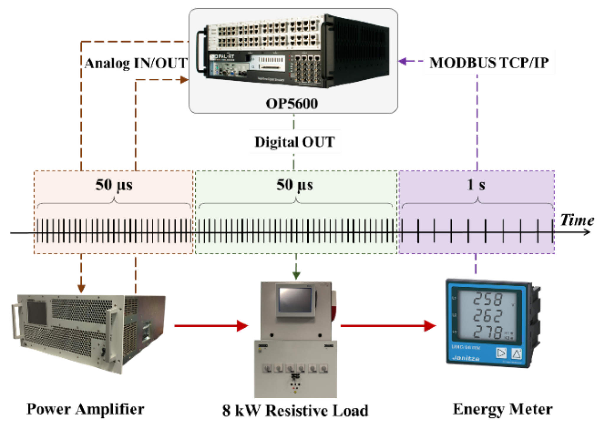
Figure 4.
Voltage reference signal transmitted from the OP5600 to the amplifier as input.

Figure 5.
Experimental results for scenario with a 2.2 kW consumption rate: (A) voltage; (B) current.
Figure 5.
Experimental results for scenario with a 2.2 kW consumption rate: (A) voltage; (B) current.

Figure 6.
Results of regression calculation considering each load level and various frequencies.

Figure 7.
Error using regression of voltage: (A) average; (B) maximum and minimum.

Figure 8.
Error using regression of frequency: (A) average; (B) maximum and minimum.

Table 1.
Values parameters sent to the amplifier for each load level.
| ID | Parameters | Step Size | Parameter Variation | Number of Steps | ||
|---|---|---|---|---|---|---|
| Min | Setpoint | Max | ||||
| A1 | Voltage Amplitude 1 (V) | 2.6% | 184 | 230 | 250 | 11 |
| A2 | Voltage Amplitude 2 (V) | 2.6% | 184 | 230 | 250 | 11 |
| A3 | Voltage Amplitude 3 (V) | 2.6% | 184 | 230 | 250 | 11 |
| F1 | Frequency phase 1 (Hz) | 49 | 50 | 51 | 5 | |
| F2 | Frequency phase 2 (Hz) | 1% | ||||
| F3 | Frequency phase 3 (Hz) | |||||
| PA1 | Phase Angle 1 (rad) | 0% | - | 0 | - | 1 |
| PA2 | Phase Angle 2 (rad) | 0% | - | 2π/3 | - | 1 |
| PA3 | Phase Angle 3 (rad) | 0% | - | −2π/3 | - | 1 |
| Total Number of Scenarios | 6655 | |||||
| Number of Scenarios with A1 + A2 + A3 ≤ 690 V | 3355 | |||||
Table 2.
Quantity of obtained data in the case study for each load level.
| Load Value | Number of | ||
|---|---|---|---|
| Expected Data | Actual Obtained Data | ||
| Before Cleaning | After Cleaning | ||
| 2.20 kW | 16,775 | 15,302 | 11,533 |
| 1.70 kW | 16,775 | 14,239 | 9657 |
| 1.30 kW | 16,775 | 14,495 | 8889 |
| 0.85 W | 16,775 | 14,445 | 8621 |
| 0.40 W | 16,775 | 14,516 | 8415 |
Table 3.
The regression equation for each load and frequency level based on the obtained results.
| Load Rate (kW) | Frequency Rate (Hz) | Regression Approach (A) | Regression Approach (B) |
|---|---|---|---|
| 2.2 | 49.0 | PSUM = 5.834 VSUM − 1832.2 | PSUM = 5.8326 VSUM − 1833.9 |
| 49.5 | PSUM = 5.8481 VSUM − 1845.1 | ||
| 50.0 | PSUM = 5.8396 VSUM − 1838 | ||
| 50.5 | PSUM = 5.796 VSUM − 1811.5 | ||
| 51.0 | PSUM = 5.8357 VSUM − 1836.4 | ||
| 1.7 | 49.0 | PSUM = 4.6088 VSUM − 1420.2 | PSUM = 4.6815 VSUM − 1467.2 |
| 49.5 | PSUM = 4.6727 VSUM − 1463.2 | ||
| 50.0 | PSUM = 4.7302 VSUM − 1499.1 | ||
| 50.5 | PSUM = 4.6973 VSUM − 1477.3 | ||
| 51.0 | PSUM = 4.6975 VSUM − 1475.9 | ||
| 1.3 | 49.0 | PSUM = 3.352 VSUM − 1010.9 | PSUM = 3.4497 VSUM − 1074.4 |
| 49.5 | PSUM = 3.4511 VSUM − 1076.4 | ||
| 50.0 | PSUM = 3.5123 VSUM − 1114.3 | ||
| 50.5 | PSUM = 3.4652 VSUM − 1084.4 | ||
| 51.0 | PSUM = 3.4772 VSUM − 1092.2 | ||
| 0.85 | 49.0 | PSUM = 2.2676 VSUM − 699.77 | PSUM = 2.3134 VSUM − 729.2 |
| 49.5 | PSUM = 2.3227 VSUM − 735.76 | ||
| 50.0 | PSUM = 2.3342 VSUM − 742.5 | ||
| 50.5 | PSUM = 2.3189 VSUM − 733.66 | ||
| 51.0 | PSUM = 2.3261 VSUM − 738.53 | ||
| 0.40 | 49.0 | PSUM = 1.1281 VSUM − 348.87 | PSUM = 1.1443 VSUM − 359.24 |
| 49.5 | PSUM = 1.1473 VSUM − 360.92 | ||
| 50.0 | PSUM = 1.1494 VSUM − 362.94 | ||
| 50.5 | PSUM = 1.1405 VSUM − 356.68 | ||
| 51.0 | PSUM = 1.1569 VSUM − 367.41 |
Table 4.
Regression measures.
| Chart in Figure 6 | m | c | r2 |
|---|---|---|---|
| (A) | 5.8326 | −1833.9 | 0.9576 |
| (B) | 4.6815 | −1467.2 | 0.9475 |
| (C) | 3.4497 | −1074.4 | 0.9419 |
| (D) | 2.3134 | −729.2 | 0.9495 |
| (E) | 1.1443 | −359.2 | 0.9449 |
Disclaimer/Publisher’s Note: The statements, opinions and data contained in all publications are solely those of the individual author(s) and contributor(s) and not of MDPI and/or the editor(s). MDPI and/or the editor(s) disclaim responsibility for any injury to people or property resulting from any ideas, methods, instructions or products referred to in the content. |
© 2022 by the authors. Licensee MDPI, Basel, Switzerland. This article is an open access article distributed under the terms and conditions of the Creative Commons Attribution (CC BY) license (https://creativecommons.org/licenses/by/4.0/).
Share and Cite
MDPI and ACS Style
Faria, P.; Vale, Z. Realistic Load Modeling for Efficient Consumption Management Using Real-Time Simulation and Power Hardware-in-the-Loop. Energies 2023, 16, 338. https://doi.org/10.3390/en16010338
AMA Style
Faria P, Vale Z. Realistic Load Modeling for Efficient Consumption Management Using Real-Time Simulation and Power Hardware-in-the-Loop. Energies. 2023; 16(1):338. https://doi.org/10.3390/en16010338
Chicago/Turabian StyleFaria, Pedro, and Zita Vale. 2023. "Realistic Load Modeling for Efficient Consumption Management Using Real-Time Simulation and Power Hardware-in-the-Loop" Energies 16, no. 1: 338. https://doi.org/10.3390/en16010338
Note that from the first issue of 2016, this journal uses article numbers instead of page numbers. See further details here.