


Stochastic Programming Model Integrating Pyrolysis Byproducts in the Design of Bioenergy Supply Chains

Mechanical Engineering Department and Texas Sustainable Energy Research Institute, The University of Texas at San Antonio, One UTSA Circle, San Antonio, TX 78249, USA
*
Author to whom correspondence should be addressed.
Energies 2023, 16(10), 4070; https://doi.org/10.3390/en16104070
Submission received: 29 March 2023
/
Revised: 4 May 2023
/
Accepted: 9 May 2023
/
Published: 13 May 2023
(This article belongs to the Special Issue Bio-Waste to Energy and Added Value Products – Challenges and Opportunities)
Abstract
:Biomass is an abundant resource for energy production and it has gained attention as a mainstream option to meet increasing energy demands. Pyrolysis has been one of the most prevalent thermochemical processes for biomass conversion. In the pyrolysis process, the biomass decomposes into three byproducts: bio-oil (60–75%), biochar (15–25%), and syngas (10–20%), depending on the feedstock and its composition. The energy required to convert the biomass varies depending on the levels of cellulose, hemicellulose, and lignin. This work proposes a novel two-stage stochastic model that designs an efficient biomass supply chain mindful of the trade-offs between pyrolysis byproducts (bioethanol and biochar). Remarkably, the model integrates biomass quality-related costs associated with moisture and ash content such as the energy consumption of preprocessing equipment and boiler maintenance due to excess ash. Biomass quality directly affects the production yield as well as the total cost of production and distribution. The results from our case study indicate a shortage of biomass from the suppliers to fulfill the demand for biochar from the power plants and bioethanol from the cities. Furthermore, the bioethanol price has the most impact on the total supply chain according to our sensitivity analysis.
1. Introduction
Due to its high economic feasibility, attributed to its high energy density and transportability, petroleum dominates the transportation energy market [1]. However, many factors, including increasing population, have given rise to the demand for a sustainable alternative [2]. Greenhouse gas emissions from the burning of fossil fuels negatively affect the quality of living due to factors such as climate effects [2,3,4]. In light of this, fuels derived from biomass (e.g., bioethanol) offer a promising alternative. In 2019, according to the Energy Information Administration, only 12% of the total energy production was derived from renewable resources [5]. However, The Renewable Fuel Standard (RFS) was enacted under the Energy Independence and Security Act, which mandates a minimum volume of renewable fuels [6]. Its revision, the RFS2, aims for 36 billion gallons per year (BGY) of biofuels to be produced for the consumption of domestic (US) transportation fuel by 2022. In addition to bioethanol, there are other energy products that can be derived from processing biomass (biochar and biodiesel, among others). The utilization of multiple energy products is a crucial step in achieving cost-competitive biomass supply chain (SC) networks. Among biofuels, a distinction can be made between them based on their sources. First-generation biofuels are derived from crops such as corn and sugarcane and second-generation biofuels are made from non-edible crop residues such as corn stover, wheat straw, energy crops, and municipal waste. While the former currently dominates the biofuel market, it is not without its drawbacks. The sourcing of first-generation biofuels directly competes with the food supply. Second-generation fuels do not exhibit this issue but are plagued with their own unique challenges, namely low energy density resulting in high transportation costs. With this in mind, a second-generation biofuel SC should incorporate preprocessing facilities in addition to tactically activated suppliers and placed biorefineries in order to strive to be cost-competitive with petroleum. Simply contracting suppliers in close proximity to biorefineries is not sufficient for the bioethanol supply to meet the market demand. More remote suppliers should be incorporated and transportation hubs, along with cheap travel options such as railroads, should be introduced to address the transportation costs. In the production of biofuels, some important physical and chemical characteristics must be accounted for. Specifically, the moisture content of the biomass increases its weight resulting in higher transportation costs. Additionally, conversion technologies are affected by the moisture and ash content of the biomass. For example, in the thermochemical conversion process, high levels of moisture content can significantly impact the process. Higher levels of moisture require more heat to remove them from the biomass; therefore, more energy is required in the conversion process [7]. Additionally, another key characteristic of biomass is the ash content in high concentrations. The ash accumulates in the boiler at a faster rate [7], which negatively affects the efficiency of the process [8]. The natural variability in these two quantities, moisture, and ash content are key considerations in developing a resilient biomass SC. Biomass densification and preprocessing are commonly employed methods to reduce this variability. Densification involves drying the biomass, generally at a depot, which results in smoother conversion, due to less moisture variability, as well as lowered transportation costs from the depot to the biorefinery. The proposed model utilizes this concept to lower transportation costs and also reflects the natural variability found in biomass moisture and ash content. As for the conversion technology, the proposed model utilizes pyrolysis. Pyrolysis is the process of heating organic material, such as biomass, at high temperatures in the absence of oxygen [9]. Due to the lack of oxygen, the organic material does not combust. Instead, the process decomposes into combustible gases and charcoal. In addition to the utilization of depots to facilitate cost-competitive biofuel production, the present work makes use of three biomass pyrolysis byproducts (bioethanol, biochar, and biodiesel) in order to raise the unit value of raw biomass to encourage additional fuel production.
1.1. Literature Review
Linear programming models are often utilized in the modeling of biomass supply chains. Ref. [10] present a model that makes use of a Geographic Information System (GIS) approach to determine the optimal location of biomass suppliers in relation to torrefaction plants and gasification facilities. Inter-facility resource competition and variable biomass pricing were the main model considerations. The model’s objection function sought to minimize the marginal costs related to the supply of torrefied wood to the gasification plants to determine the plants’ locations. Dijkstra’s algorithm is used to find the shortest route between forest sites and torrefaction plants to determine the allocation of existing biomass supply. This paper differs from this approach in that it determines the optimal location of biorefineries and depots rather than focusing on biomass supply. Other implementations of linear programming in relation to biomass supply chains seek to implement the uncertainty in regard to transportation when designing depots [11]. In Cundiff, Dias, and Sherali [11], supply uncertainty is explained by four growing season and harvest month weather scenarios. The scenarios are then used in a multi-stage LP model to determine the cost and optimal size of monthly inter-facility biomass shipments. This concept of using weather to influence supply chain uncertainty is of vital importance when dealing with cost optimization as it pertains to biomass. The variable growing conditions directly affect the characteristics of the supply and should not be overlooked when seeking to formulate optimization models for biomass supply chains. The complex interactions between biomass logistics and supply chain design and the desire to simultaneously optimize facility locations and biomass supply flow have motivated many authors to utilize mixed integer linear programming [12,13,14,15,16]. Bowling and El-Halwagi [17] structure their biomass supply chain as a network with nodes containing locations such as suppliers, pretreatment sites, and conversion facilities and the arcs are the transportation between them. Within the MILP, binary variables are utilized to determine whether or not facilities are constructed at a particular location and continuous decision variables are used to describe the biomass flow. The model was optimized based on economic, environmental, and energetic objectives and considered constraints that included things such as capacities, demands, and mass balances. Our proposed model structure is very much in line with the aforementioned model, specifically the network design. Recently, major logistics improvements within targeted strategic areas within biomass supply chains have been proposed and have the potential to increase the economic feasibility of consumer utilization of biofuels. Namely, the moisture and ash content of biomass and their effect on supply chain logistics. To incorporate these quantities into supply chain decisions, researchers often turn to two-stage stochastic programming models. Castillo et al., 2017 [18], make use of trust region cuts and multi-cuts to solve a two-stage stochastic model to determine the optimal or near-optimal location of biorefineries and their associated conversion technologies under the uncertainty that accompanies biomass moisture content. Another innovation in biomass supply chain networks has been the introduction of depots to preprocess and condense biomass prior to transportation to biorefineries. The key advantages of this approach are twofold. First, the preprocessing of biomass offers a level of physical and chemical consistency that in turn reduces the variability associated with the conversion of raw biomass into biofuels. Second, the densification and drying that takes place in depots and their proximity to suppliers and mass transportation railways has the potential to reduce total SC transportation costs. Aboytes-Ojeda et al., 2018 [19] introduce a two-stage stochastic model that uses a hub-and-spoke network, including depots that preprocess biomass. In addition to moisture variability, the model also considers the natural variability in biomass ash content when determining the depots’ locations, biorefineries locations, selection of conversion technologies, and the biomass required for bioethanol production. The impact of moisture and ash variability on supply chain decisions was demonstrated by performing a case study in Texas. Moreover, closely related to the present work is that the aforementioned model made use of the L-shaped (LS) method to obtain a near-optimal solution with reasonable computation time. Numerous examples of using the LS method, among others, to solve large-scale optimization problems can be found in the literature. For example, Marufuzzaman et al. [20] introduce a two-stage stage stochastic model to design and manage a biodiesel supply chain. The solution approach was implemented to solve a case study in the state of Mississippi utilizing a hybrid method between Lagrangian relaxation and the L-shaped method. The present work distinguishes itself from the above by utilizing the LS method for a byproduct (biochar and bioethanol) biomass supply chain to explore more complex interactions. The conversion technology for biomass in the present work is fast pyrolysis. Fast pyrolysis takes raw biomass and converts it to bio-oil, biochar, and syngas. Supply chains incorporating this conversion technology should seek to make use of more than one of these byproducts rather than focusing on just bio-oil. Casler and Boe, 2003 [21] demonstrate that pyrolysis was a more effective means of conversion than co-firing for meeting the electricity demands of Taiwan. Additionally, the authors made use of bio-oil to meet electricity demands and biochar was used as a soil additive to increase crop yields in Taiwanese farms. In contrast, the present work seeks to use biochar to meet coal plant demands rather than as a soil additive. The categorization of the reviewed previous works is summarized below in Table 1.
1.2. Contributions
The present work proposes a model that fills a gap in the literature and advances the field of bioenergy supply chain network design by considering the random nature of the biomass quality-related properties, the investment and operational costs, and the trade-off between bioethanol and biochar alongside the utilization of biodiesel to design a supply chain network that minimizes the overall cost of fulfilling the bioethanol demand for cities and the biochar demand from power plants. The contributions of this work can be categorized as modeling and application. Regarding modeling, in the proposed two-stage stochastic formulation, the variability of moisture and ash content are taken into account when considering the total cost of producing biofuels and how they affect the design of the SC based on [19]. The unique feature is that the model utilizes three distinct pyrolysis byproducts where two (bioethanol and biochar) are used to meet realistic demands and biodiesel is fed back into the SC in order to reduce the cost of producing the former. The model aims to minimize investment, transportation, and quality-related costs given a selection of the conversion technologies, the number of facilities (depots, biorefineries, power plants, and cities), and their locations. From the application standpoint, a realistic comprehensive case study in Texas, the native home of the Alamo cultivar of switchgrass, is utilized to test the model and obtain managerial insights into the management and planning of the biomass supply chain (SC).
2. Mathematical Model
A hub-and-spoke network model consisting of five sets of nodes was used for the formulation of this problem. The first set of nodes represents the counties, the second set represents the potential locations for depots/hubs where consolidation and densification of the biomass occurs, the third set represents the potential locations for biorefineries, the fourth and fifth sets represent the cities and power plants to which the pyrolysis byproducts supply, respectively. A hub-and-spoke model with 4 suppliers, 3 depot facilities, 2 biorefineries, 1 city, and 1 power plant is illustrated in Figure 1 The network consists of the current links between counties and depots while it also considers the possible connections between depots and biorefineries. By setting the densification process in the depots instead of counties, the resulting effect is that no connections are established between counties and biorefineries. Before every shipment of biomass is shipped to the corresponding biorefinery, it must first stop at a depot for the densification process.
The dynamics of this model consist of trucks delivering biomass from counties to depots, while unit trains deliver from depots to biorefineries. The transportation costs of utilizing trucks are associated directly with the distance between the origin and destination points. On the contrary, rail transportation is priced according to the distance between depots and biorefineries along with the cost of loading and unloading the unit train. The work of Roni [22] introduces a unit train as a set of cars that usually transports one type of product from one location to the destination without any further stops for additional loading/unloading. This method of transportation offers a cost-efficient solution for the delivery of high-volume products directly to the customer. Trucks are used to transport the pyrolysis byproducts to the cities (biofuel) and the power plants (biochar) from the biorefineries.
The model includes the following assumptions. Firstly, pyrolysis will yield three byproducts (bioethanol, biodiesel, and biochar). Secondly, although biochar can have multiple uses, such as being a soil additive that greatly increases the health of the soil, its production will be used solely to fulfill the demand of 17 coal power plants around Texas for the production of electricity. Thirdly, the pyrolysis bioethanol will be used to supply the bioethanol demand of Houston, Dallas, San Antonio, Austin, Plano, Fort Worth, El Paso, Arlington, Corpus Christi, and Laredo. Lastly, biodiesel will be used to reduce the transportation cost of products leaving the refinery.
The description and formulation of the hub-and-spoke model are presented next:
Sets:
- : Nodes of distribution network , for all .
- : Arcs of distribution network , for all .
- : Set of counties(suppliers) for all .
- : Set of potential locations for depots, for all .
- : Set of potential locations for biorefineries, .
- : Set of power plants (coal), .
- : Set of cities, .
- : Set of arcs from to , .
- : Set of arcs from to , .
- : Set of arcs from to , .
- : Set of arcs from to , .
- : Set of technologies for conversion, .
- : Set of scenarios, .
Parameters:
- : Investment cost to open a depot at node .
- : Investment cost to open a biorefinery at location utilizing technology .
- : Fixed cost of loading/unloading a unit train along arc every week for a period of one year (52 weeks).
- : Unit transportation and procurement cost charged per metric ton shipped along arc .
- : Total unit cost charged per metric ton shipped along arc .
- : Fixed unit cost charged per metric ton shipped along arc .
- : Fixed unit cost charged per metric ton shipped along arc .
- : Variable unit cost charged per metric ton per kilometer along arc .
- : Variable unit cost charged per liter per kilometer along .
- : Distance of arc (kilometers) .
- : Distance of arc (kilometers) .
- : Represents the penalty cost for demand shortage of coal.
- : Represents the penalty cost for demand shortage of bioethanol.
- : Represents the monetary value per liter of biodiesel.
- : Conversion factor for biomass/biochar supplied to power plant applying pyrolysis.
- : Conversion factor for biomass pyrolysis oil to bioethanol.
- : Conversion factor for biomass pyrolysis oil to biodiesel.
- : Maximum capacity of a unit train along arc .
- : Represents the preprocessing capacity of depot facility .
- : Production capacity of biorefinery including technology .
- : Distance from biorefinery to power plant.
- : Distance from biorefinery to city.
- : Total demand of biochar.
- : Total demand of bioethanol.
- : Byproduct share of biochar.
- : Byproduct share of bio-oil.
- : Total unit cost charged per metric ton shipped along arc under scenario .
- : Available supply in county for scenario .
- : Probability of scenario .
Quality-related Parameters:
- : Target moisture content of conversion technology.
- : Target ash content of conversion technology.
- : Boiler maintenance cost.
- : Densification cost at .
- : Cooling cost at .
- : Electricity cost at .
- : Grinding loss in stage 1 at .
- : Grinder feed rate at .
- : Moisture-related cost under scenario for a given .
- : Grinding cost under scenario .
- : Energy consumption due to the grinder at by processing biomass delivered from farm .
- : Moisture content of biomass coming from farm for scenario .
- : Energy consumption due to the rotary shear at .
- : Moisture content of biomass after grinder at .
- : Biomass screen size after grinder at under scenario .
- : Ash removal and disposal cost under scenario for a given .
- : Ash content of biomass coming from county for scenario .
Variables:
- : A binary variable, which takes the value 1 if a depot is connected with a biorefinery , and 0 otherwise.
- : A binary variable which takes the value 1 if if the potential location is used as a biorefinery utilizing technology , and 0 otherwise.
- : A binary variable which takes the value 1 if potential location is used as depot, and 0 otherwise.
- : Flow along arc under scenario .
- : Flow along arc under scenario .
- : Flow along arc under scenario .
- : Flow along arc under scenario .
- : Variable cost incurred by product shipped along arc after diesel related cost reduction under scenario .
- : Variable cost incurred by product shipped along arc after diesel related cost reduction under scenario .
- : Quantity of biodiesel allocated to shipping cost reduction along arc under scenario .
- : Quantity of biodiesel allocated to shipping cost reduction along arc under scenario .
- : Third party coal supply under scenario .
- : Third party bioethanol supply under scenario .
Now, we proceed with the mathematical formulation. Note that depot and biorefinery location selection, as well as unit train contracting (, , ), are known as first-stage decisions. Meaning that they are made prior to the realization of a stochastic event (supply and moisture/ash content). However, once the stochasticity is imposed through representative scenarios, the second-stage decisions such as biomass allocation (, ), byproduct allocation (, ), and diesel allocation (, , , ), as well as demand shortages (, ), can be made.
The objective function is the minimization of the total cost as shown in (1), which consists of infrastructure investment, logistics operations, and biomass purchase. The first two terms in (1) denote the investment costs for opening depots and biorefineries, while the third term contains the costs of unit train contraction. The remaining terms contain information on biomass transportation, procurement and conversion costs, and demand shortage penalty costs. These terms are manifested as the weighted sum over a set of scenarios aimed at capturing the uncertainty in supply and moisture/ash content. The model is restricted by the following constraints.
Constraints (2)–(5) are capacity constraints. With (2) ensuring the total amount of biomass acquired from a county cannot exceed the available supply. This denotes the first manifestation of uncertainty as the supply varies over the different scenarios. Equations (3) and (4) ensure deport and biorefinery capacities are not exceeded in the event that a facility is opened and prevent commodity flow into unopened facilities. Equation (5) ensures unit train capacity is not exceeded.
Constraints (6)–(8) are mass conservation constraints. Equation (6) ensures that the amount of raw biomass minus its moisture content entering each depot is exactly equal to the amount of densified dry biomass exiting the facility. Stochasticity is again at play here due to the varying moisture content . Equations (7) and (8) ensure the fuel byproducts leaving a refinery are the same as biomass flowing into a refinery times a conversion coefficient.
Constraints (9) and (10) enforce demand satisfaction by allowing and to compensate for the failure of byproducts and to meet demands and .
Constraints (11) and (13) pertain to the utilization of biodiesel to reduce transportation costs in the network. Equation (11) ensures the amount of diesel utilized does not exceed the amount produced. Equations (12) and (13) utilize new decisions and to denote the variable shipping cost not offset by biodiesel allocation for trucks leaving biorefineries.
Constraints (14)–(26) are domain constraints that ensure non-negativity in mass flows and resource allocation as well as enforce the binary nature of stage one decisions.
Costs along Arc
Costs incurred along arc include the transportation per unit and the biomass procurement costs, as well as the depot preprocessing costs, which include moisture and ash penalty terms. The total cost is given in the following equation:
Random levels of moisture and ash content directly affect the quality-related costs denoted by and , respectively. For example, if the biomass contains high levels of moisture and ash, then additional operations will be required to meet the desired composition for conversion. In this work, the densification process consists of four operations: grinding stage 1, grinding stage 2, densification, and cooling. The energy required to grind biomass with high levels of moisture is larger and therefore more costly. Additionally, boiler maintenance is affected by the ash content in the biomass. Since it is necessary to remove the ash residue adhered to the boiler after conversion, higher levels of ash lead to higher maintenance costs. The energy requirements of the grinder (grinding stage 1) and the rotary shear (grinding stage 2) are estimated using expressions (30) and (31), respectively. The energy and overall moisture-related costs are calculated using expressions (29) and (28), respectively [18].
3. Case Study
Located in the southern region of the United States, Texas has the potential infrastructure and locations to build an SC capable of producing and distributing bioethanol (derived from bio-oil) along with other byproducts. Features such as railroad connectivity and biorefinery locations provide the necessary tools for a potential supply chain in Texas. Furthermore, one of the primary feedstocks proposed by the Idaho National Laboratory to produce bioethanol is switchgrass [23] and Texas has the potential to produce this type of feedstock. The next sub-sections present the data collection methods.
3.1. Biomass Supply
This case study utilizes all 254 counties in the state of Texas [24] as the biomass suppliers. Every county in this case study considers the following characteristics:
- The available biomass.
- The biomass moisture content.
- The biomass ash content.
- The weather condition scenario.
The supply of dry biomass for every county in Texas for 2021 was collected utilizing the Billion-Ton Report [25]. The scenarios for the stochastic programming model consider the characteristics described before. The steps to generate the scenarios are introduced in the next section.
3.2. Scenario Generation
The scenario generation utilizes the following procedure:
- Gather historical data of the daily precipitation level of every county.
- Use the historical data to estimate the weighted average yearly precipitation for every county.
- Depending on the levels of daily precipitation, a county is classified as humid or dry. If the value is above average, the county is considered humid and vice-versa.
- Calculate the frequency of a county’s humid conditions for harvesting.
- Set the number of scenarios.
- Generate n random numbers to classify a county as humid or dry. A random number above the probability assigns a county as dry and a lower number assigns a county as humid.
- The moisture content of a humid county is sampled from the right-hand side of the triangular distribution and vice-versa.
- The triangular distribution is used to generate a random ash content.
The concentration levels of moisture and ash in the biomass are used to calculate the processing costs. This work utilizes the daily precipitation data from 1991 to 2011 according to the CDC Wonder [26]. Furthermore, the weighted average is determined according to the number of observations recorded by a county throughout the year. Following the work of Aboytes et al. [19], the moisture and ash content for each county under each scenario are derived from triangular distributions centered at 17.5% and 10%, respectively, with minimum values of 14.5% and 5% as well as maximum values of 26.50% and 15%.
3.3. Depots
This work considers train stations as the candidates to set up depot facilities; therefore, the potential depot locations were obtained from a shape file from Oak Ridge National Laboratory [28]. The following heuristic defined the set of potential candidates for depot locations; the supply provided by the county was used to determine its sort order and then associated with the closest train station. Figure 2 shows the thirty-three train stations considered in the set of potential locations. The depot attributes consist of two parameters: the preprocessing capacity for the depot and the investment cost to open a depot facility. To open a depot facility, the total capital investment (TCI) required is $21,758,808 USD [29] with an equivalent annual cost (EAC) of $3,476,219 USD utilizing an interest rate (r) of 15% and an estimated lifetime of the project (t) of 20 years. For conventional pelleting process depots, the preprocessing capacity is 300,000 Mg/year [29]. However, to match the large-scale model proposed in this thesis, the capacity was scaled up utilizing linear estimation.
3.4. Biorefineries
The potential locations for biorefineries were obtained from the Bioenergy Atlas site [30]. Once a suitability analysis was conducted, it was determined that there are 167 potential biorefinery locations (Figure 2). The TCI to open a biorefinery with biomass pyrolysis technology is $819,702,000 USD [31] with EAC of $130,956,797 USD (r = 15%, t = 20 years for both technologies). The production capacity is 804,825 Mg/year [31]. In pyrolysis, the biomass decomposes into three byproducts, which include bio-oil (58%), biochar (20%), and syngas (17%) depending on the feedstock [32]. In addition, the bio-oil is further processed to produce bioethanol and biodiesel with conversion factors 236 liters/Mg oil and 258 liters/Mg oil, respectively [31]. On top of the investment cost, the biorefineries are also assigned a mix of operational costs and processing costs shown in Table 2. The fixed costs are added to the EAC in the model and the variable costs are included in that parameter , which is multiplied by the quantity of densified biomass entering the refinery.
3.5. Transportation and Other Costs
The Open Source Routing Machine was used to generate the distance for every arc , arc , and [33]. For arc , the distance was generated with a local application in R software environment [34]. The cutoff point in the arcs that connect the set of counties with the depots is 170 km. It is not recommended to ship biomass using trucks for long distances; therefore, a greater distance than 170 km between the origin-destination is not included in set [35]. The transportation costs come in the form of linear regression results and thus are split into a fixed cost (Table 3) and a variable cost (Table 4) where the latter is multiplied by the distance traveled. All costs are per unit product shipped and thus fluctuate based on how much product is routed along each arc.
It is worth reiterating here that the biodiesel produced in the SC offsets the variable transportation costs along arcs and with a monetary value of $0.68 per liter. Also of note is that the fixed transportation cost for arc is very low. This is due in part to utilizing unit trains in lieu of trucks but also because the fixed cost for loading and unloading the unit trains appears elsewhere in the model. This practice is in agreement with the work conducted by Roni [22].
3.6. Power Plants
The demand for biochar was derived from ten percent of the total energy produced by 17 coal plants in Texas [30]. Utilizing the fuel heat content of coal (BTU) and the tons of coal required to produce one MhW of power the demand is expected to be 5.41 million tons. Additionally, according to the EIA, the average coal price per metric ton was 33.72 [38]. This is the penalty cost for failing to meet the in-state coal demand with biocoal. The locations are shown in Figure 3.
3.7. Cities
The expected biofuel demand for Texas is approximately 5.6 billion liters of bioethanol [39]. However, this model only considers the top eight most populous cities in Texas, which represents about 30% of the total population [40]. As a result, the model considers 1.7 billion gallons of bioethanol as the demand. A penalty cost of $2.80 USD per liter of bioethanol is used to force the required level of in-state bioethanol production. In this work, the same penalty cost is considered and the realization probability for every scenario is equally distributed (i.e., all the scenarios have the same probability). The locations are shown in Figure 3.
4. Results
In this section, a numerical representation analysis of the Texas case study is presented. It should be noted that only one technology (pyrolysis) is considered. The case study was conducted on a computer with a processor Intel(R) Core(TM) i9-7980XE CPU @ 2.60 GHz and 32 GB of RAM. Additionally, the IBM ILOG CPLEX 12.8.0 with built-in Benders Decomposition was used to find the optimal solution for our model within a gap of 2.5%.
4.1. Numerical Results
The total cost associated with the hub-and-spoke network is $4,835,050,875 USD with the investment and operational cost (I&OP) being $2,932,084,423 USD. The largest cost is the initial investment of opening the biorefinery at 70% of the I&OP cost. Transportation and handling cost for biomass and byproducts is 27% and the cost of opening depots is 3% of the I&OP cost. The optimal SC selected 33 out of the 33 potential depot locations and 10 out of the 167 potential biorefinery locations. There are 20 different scenarios that consider varying quality for our optimal solution. The primary reason why 20 scenarios is an appropriate number is that we want to have enough scenarios to capture the natural variability of the biomass; however, we also want to minimize the computational effort and time in attaining an optimal solution. Running too many scenarios will significantly increase the solution time. Based on the results obtained, the SC’s inability to fulfill the coal demand for the power plants and bioethanol demand from the cities results in $1,902,966,452 USD in third party costs, and this accounts for 39% of the overall costs as shown in Figure 4.
4.2. Sensitivity Analysis
A sensitivity analysis was performed on the third-party pricing of biochar and bioethanol, where each penalty cost was varied from the case study value while the other was fixed at that value. This was performed to better understand which commodities have the largest impact on BSC design. The results are shown in Figure 5.
We observe that no change in production is observed when the biochar price is altered. Further analysis indicates that even a 300% increase and 50% decrease in biochar price do not affect the biomass processed. However, a 1.5% decrease in ethanol penalty costs is enough to lower the amount of biomass processed, and a 7% decrease results in a scenario where production is not desirable. In addition, a 40% increase does not cause the model to process more biomass than was processed in the case study. From this sensitivity analysis, it can be concluded that for the third-party pricing in the case study, the model is running at maximum feasible capacity, which is corroborated by the observed 8,050,000 MG biomass processed being exactly the sum of the 33 depot capacities. Additionally, ethanol pricing has the largest impact on production levels.
As for the minimum required third-party pricing for bioethanol to force production, Figure 6 shows the breakdown of how much of each aspect of the SC contributes to the cost.
The costs shown assume that the depot, unit train, and bio-refinery that this liter passed through are running at full capacity. If they are not, then the costs shown will increase. In addition, variable shipping costs, as well as quality penalty costs, are not included and combined bridge the gap between the price shown in Figure 6 and the value present in the model.
In conclusion, the model is more sensitive to bioethanol pricing than it is to biochar pricing. In addition, the high bioethanol price can be mostly explained by the investment and operational costs of the pyrolysis biorefineries selected for the SC.
5. Conclusions and Future Work
In this research, we developed a stochastic programming model integrating pyrolysis byproducts in the design of biomass supply chains. The model considered the multi-modal transportation of biomass. A unit train was considered as a method to transport high-volume batches between depots and biorefineries, while a truck was utilized to transport biomass from suppliers to depots and from biorefineries to the customer. The model included quality-related costs associated with the feedstock properties such as moisture and ash content. This is important to consider given that these properties directly affect the logistic operation of the biomass SC, the production yield, and the total cost of production and distribution. The model’s objective was to minimize the cost of facility location, transportation, and distribution of biomass and pyrolysis byproducts. It is important to note that the results from our case study indicate that depot capacity leads to an inability for the SC to fulfill the demand for biochar from the power plants and bioethanol from the cities. However, it is important to consider that biochar was utilized as a substitute for all the electricity generated from coal in Texas. As a result, there will be an insufficient supply of biomass to completely substitute the generation of electricity from coal if 58% of the biomass supply yields bioethanol given the pyrolysis conversion process. Hence, the model is driven by the bioethanol price according to our sensitivity analysis. In addition, the biodiesel was able to offset all of the variable shipping costs and was effective in reducing the price of bioethanol required to stimulate production. Future lines of research include an extension of the use of biodiesel as well as the incorporation of multiple biomass types and conversion technologies in order to produce a model that is not dominated by a single byproduct.
Author Contributions
Conceptualization, K.K.C.-V.; Methodology, K.K. and K.K.C.-V.; Investigation, K.K.; Data curation, K.K.; Writing—original draft, K.K.; Writing—review & editing, K.K.C.-V.; Supervision, K.K.C.-V.; Project administration, K.K.C.-V.; Funding acquisition, K.K.C.-V. All authors have read and agreed to the published version of the manuscript.
Funding
This material is based upon work that is supported by the National Institute of Food and Agriculture (NIFA), U.S. Department of Agriculture (USDA), under the Hispanic Serving Institutions Education Grants Program, award no. 2020-38422-32258.
Data Availability Statement
Data is available upon request.
Acknowledgments
We would like to thank Mario Aboytes-Ojeda and Luvin De Leon for their insightful discussions, which help to frame this research.
Conflicts of Interest
The authors declare no conflict of interest.
References
- EIA. Crude Oil Made into Different Fuels; EIA: Washington, DC, USA, 2019.
- Roni, M.S.; Eksioglu, S.D.; Cafferty, K.G. A Multi-Objective, Hub-and-Spoke Supply Chain Design Model for Densified Biomass. In Proceedings of the IIE Annual Conference, Montreal, QC, Canada, 31 May–3 June 2014; Institute of Industrial and Systems Engineers (IISE): Norcross, GA, USA, 2014; p. 643. [Google Scholar]
- Environmental Defense Fund. The True Cost of Carbon Solution; Environmental Defense Fund: New York, NY, USA, 2023. [Google Scholar]
- Environmental Protection Agency. Greenhouse Gases; Environmental Protection Agency: Washington, DC, USA, 2020.
- U.S. Energy Information Administration. 2020. Available online: https://www.eia.gov/energyexplained/us-energy-facts/data-and-statistics.php (accessed on 7 May 2020).
- Independence, E.; Act, S. Energy Independence and Security Act of 2007; US Government Printing Office: Washington, DC, USA, 2007.
- Brownsort, P.A. Biomass Pyrolysis Processes: Review of Scope, Control and Variability; UK Biochar Research Center: Edinburgh, UK, 2009; p. 38. [Google Scholar]
- Miles, T.R.; Miles, T., Jr.; Baxter, L.; Bryers, R.; Jenkins, B.; Oden, L. Alkali Deposits Found in Biomass Power Plants: A Preliminary Investigation of Their Extent and Nature; Technical Report; National Renewable Energy Lab.: Golden, CO, USA; Miles (Thomas R.): Portland, OR, USA; Sandia National Labs.: Livermore, CA, USA; Foster Wheeler Development Corp.: Livingston, NJ, USA; California Univ.: Davis, CA, USA; Bureau of Mines: Albany, OR, USA; Albany Research Center: Albany, OR, USA, 1995; Volume 1. [Google Scholar]
- Zhao, P.; Shen, Y.; Ge, S.; Chen, Z.; Yoshikawa, K. Clean solid biofuel production from high moisture content waste biomass employing hydrothermal treatment. Appl. Energy 2014, 131, 345–367. [Google Scholar] [CrossRef]
- Panichelli, L.; Gnansounou, E. GIS-based approach for defining bioenergy facilities location: A case study in Northern Spain based on marginal delivery costs and resources competition between facilities. Biomass Bioenergy 2008, 32, 289–300. [Google Scholar] [CrossRef]
- Cundiff, J.S.; Dias, N.; Sherali, H.D. A linear programming approach for designing a herbaceous biomass delivery system. Bioresour. Technol. 1997, 59, 47–55. [Google Scholar] [CrossRef]
- Akgul, O.; Shah, N.; Papageorgiou, L. An MILP Model for the Strategic Design of the UK Bioethanol Supply Chain. Comput. Aided Chem. Eng. 2011, 29, 1799–1803. [Google Scholar]
- Leduc, S.; Schwab, D.; Dotzauer, E.; Schmid, E.; Obersteiner, M. Optimal location of wood gasification plants for methanol production with heat recovery. Int. J. Energy Res. 2008, 32, 1080–1091. [Google Scholar] [CrossRef]
- Larkin, S.; Ramage, J.; Scurloc, J. Bioenergy. In Renewable Energy-Power for a Sustainable Future; Oxford University Press: Oxford, UK, 2004; pp. 106–146. [Google Scholar]
- Awudu, I.; Zhang, J. Uncertainties and sustainability concepts in biofuel supply chain management: A review. Renew. Sustain. Energy Rev. 2012, 16, 1359–1368. [Google Scholar] [CrossRef]
- Andersen, F.; Iturmendi, F.; Espinosa, S.; Diaz, M. Optimal design and planning of biodiesel supply chain with land competition. Chem. Eng. 2012, 47, 170–182. [Google Scholar] [CrossRef]
- Bowling, I.M.; Ponce-Ortega, J.M.; El-Halwagi, M.M. Facility Location and Supply Chain Optimization for a Biorefinery. Am. Chem. Soc. 2011, 50, 6276–6286. [Google Scholar] [CrossRef]
- Castillo-Villar, K.K.; Eksioglu, S.; Taherkhorsandi, M. Integrating biomass quality variability in stochastic supply chain modeling and optimization for large-scale biofuel production. J. Clean. Prod. 2017, 149, 904–918. [Google Scholar] [CrossRef]
- Aboytes-Ojeda, M.; Castillo-Villar, K.K.; Eksioglu, S.D. Modeling and optimization of biomass quality variability for decision support systems in biomass supply chains. Ann. Oper. Res. 2022, 314, 319–346. [Google Scholar] [CrossRef]
- Marufuzzaman, M.; Eksioglu, S.D.; Huang, Y.E. Two-stage stochastic programming supply chain model for biodiesel production via wastewater treatment. Comput. Oper. Res. 2014, 49, 1–17. [Google Scholar] [CrossRef]
- Casler, M.; Boe, A. Cultivar × environment interactions in switchgrass. Crop Sci. 2003, 43, 2226–2233. [Google Scholar] [CrossRef]
- Roni, M.S. Analyzing the Impact of a Hub and Spoke Supply Chain Design for Long-Haul, High-Volume Transportation of Densified Biomass; Mississippi State University: Starkville, MS, USA, 2013. [Google Scholar]
- Roni, M.S.; Thompson, D.N.; Hartley, D.; Griffel, M.; Hu, H.; Nguyen, Q.; Cai, H. Herbaceous Feedstock 2018 State of Technology Report; Technical Report; Idaho National Laboratory: Idaho Falls, ID, USA, 2018. [Google Scholar]
- U.S. Census Bureau. U.S. Gazetteer: 2010, 2000, and 1990; U.S. Census Bureau: Suitland, MD, USA, 2012.
- Langholtz, M.H.; Stokes, B.J.; Eaton, L.M.; Brandt, C.C.; Davis, M.R.; Theiss, T.J.; Turhollow, A.F., Jr.; Webb, E.; Coleman, A.; Wigmosta, M.; et al. 2016 Billion-Ton Report: Advancing Domestic Resources for a Thriving Bioeconomy, Volume 1: Economic Availability of Feedstocks; Technical Report; Oak Ridge National Lab. (ORNL): Oak Ridge, TN, USA, 2016. [Google Scholar]
- Centers for Disease Control and Prevention. NLDAS Daily Precipitation; Centers for Disease Control and Prevention: Atlanta, GA, USA, 2016.
- U.S. Department of Energy. 2017. Available online: https://bioenergykdf.net/billionton2016/overview (accessed on 10 May 2020).
- Center of Transportation Analysis. Railroad Network 2017. Available online: http://cta.ornl.gov/transnet/RailRoads.html (accessed on 2 May 2017).
- Lamers, P.; Roni, M.S.; Tumuluru, J.S.; Jacobson, J.J.; Cafferty, K.G.; Hansen, J.K.; Kenney, K.; Teymouri, F.; Bals, B. Techno-economic analysis of decentralized biomass processing depots. Bioresour. Technol. 2015, 194, 205–213. [Google Scholar] [CrossRef] [PubMed]
- National Renewable Energy Laboratory. 2017. Available online: https://maps.nrel.gov/bioenergyatlas (accessed on 3 March 2017).
- Jones, S.B.; Meyer, P.A.; Snowden-Swan, L.J.; Padmaperuma, A.B.; Tan, E.; Dutta, A.; Jacobson, J.; Cafferty, K. Process Design and Economics for the Conversion of Lignocellulosic Biomass to Hydrocarbon Fuels: Fast Pyrolysis and Hydrotreating Bio-Oil Pathway; Technical Report; Pacific Northwest National Laboratory (PNNL): Richland, WA, USA, 2013. [Google Scholar]
- Boateng, A.A.; Daugaard, D.E.; Goldberg, N.M.; Hicks, K.B. Bench-scale fluidized-bed pyrolysis of switchgrass for bio-oil production. Ind. Eng. Chem. Res. 2007, 46, 1891–1897. [Google Scholar] [CrossRef]
- Project-OSRM. Project-OSRM/osrm-backend. 2017. Available online: https://github.com/Project-OSRM/osrm-backend (accessed on 14 March 2017).
- R Core Team. The R Project for Statistical Computing; R Core Team: Vienna, Austria, 2017. [Google Scholar]
- Huang, Y.; Chen, C.W.; Fan, Y. Multistage optimization of the supply chains of biofuels. Transp. Res. Part E Logist. Transp. Rev. 2010, 46, 820–830. [Google Scholar] [CrossRef]
- Abbas, D.; Handler, R.; Dykstra, D.; Hartsough, B.; Lautala, P. Cost Analysis of Forest Biomass Supply Chain Logistics. J. For. 2013, 111, 271–281. [Google Scholar] [CrossRef]
- Searcy, E.; Flynn, P.; Ghafoori, E.; Kumar, A. The relative cost of biomass energy transport. Appl. Biochem. Biotechnol. 2007, 137, 639–652. [Google Scholar] [PubMed]
- EIA. Coal Prices and Outlook. In U.S. Energy Information Administration—EIA—Independent Statistics and Analysis; EIA: Washington, DC, USA, 2019. [Google Scholar]
- EIA. Texas State Energy Profile. 2019. Available online: www.eia.gov/state/print.php?sid=TX (accessed on 14 March 2018).
- Sawe, B.E. Biggest Cities in Texas. WorldAtlas 2016. Available online: https://www.worldatlas.com/cities/10-largest-cities-in-texas.html (accessed on 3 March 2017).
Figure 1.
Hub -and-spoke network.
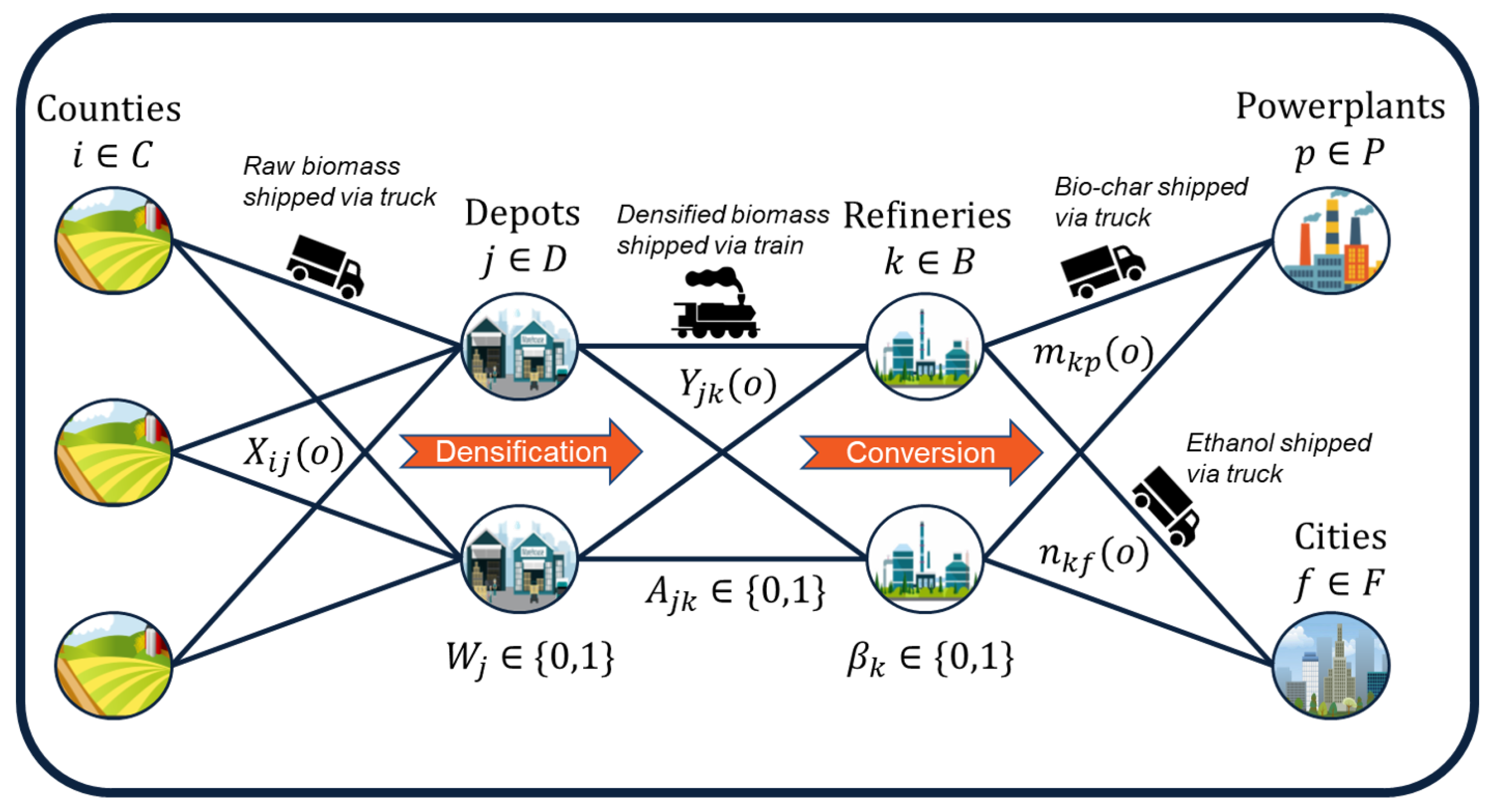
Figure 2.
Potentiallocation for biorefineries and depots in Texas.
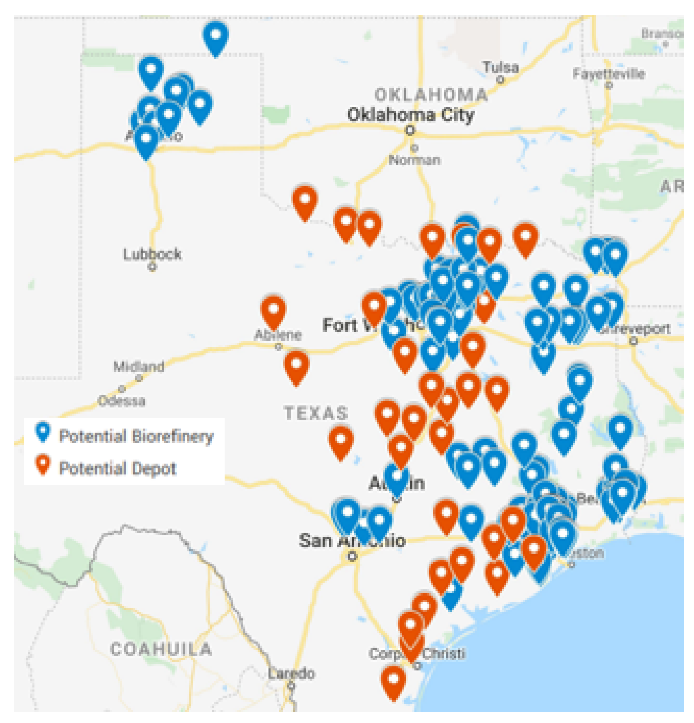
Figure 3.
Power plants and city locations.

Figure 4.
Biomass Supply Chain Breakdown of Costs.
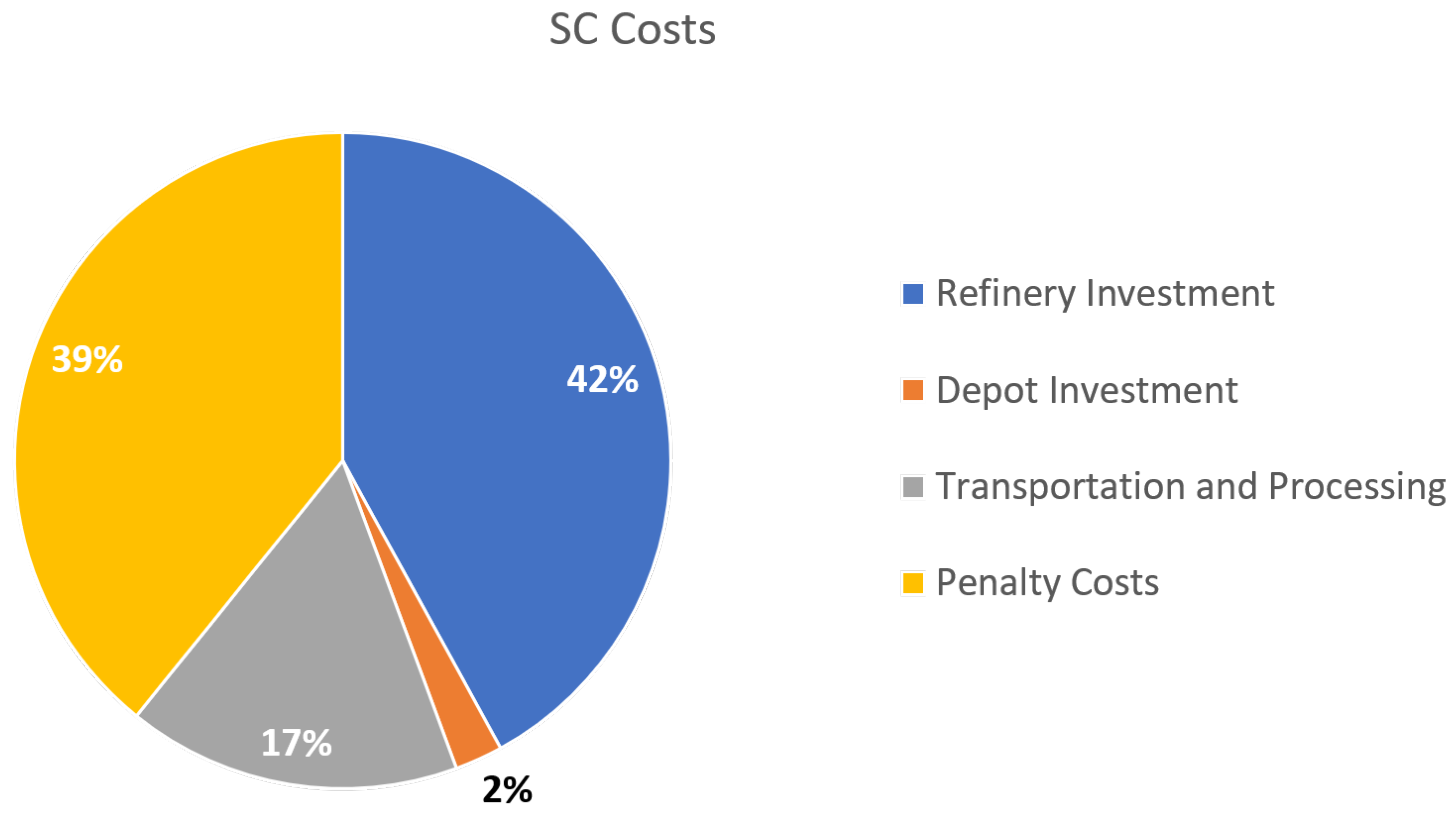
Figure 5.
Sensitivity to third party penalty costs.
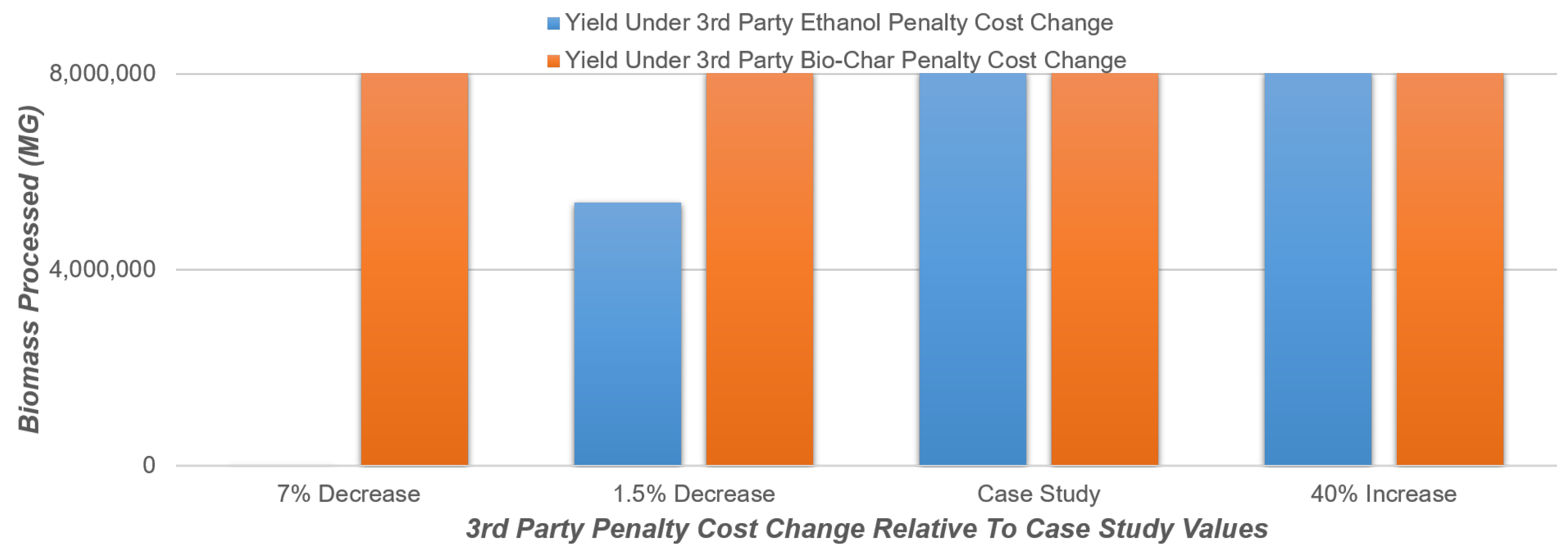
Figure 6.
Biomass Supply Chain Breakdown of Bioethanol Costs.


Table 1.
Present Model Contributions.
| Authors | Bowling, and El-Halwagi 2011 [17] | Castillo-Villar, Eksioglu, Taherkhorsandi, 2017 [18] | Aboytes-Ojeda, Castillo-Villar Eksioglu, 2018 [19] | This Work |
|---|---|---|---|---|
| Hub-and-spoke network | X | X | X | X |
| Considers variability in moisture and ash content | X | X | X | |
| Utilizes depots to reduce transportation costs and processing variability | X | X | ||
| Uses L-shape Method | X | X | X | |
| Considers multiple biomass byproducts | X |
Table 2.
Biorefinery Operational Costs.
| Cost | Type | Value | Units |
|---|---|---|---|
| Natural Gas | Variable | 10.37 | $/Mg Dry Biomass |
| Chemicals | Variable | 33.17 | $/Mg Dry Biomass |
| Waste | Variable | 1.04 | $/Mg Dry Biomass |
| Electricity | Variable | 9.32 | $/Mg Dry Biomass |
| Fixed Costs | Fixed | 39,312,000 | $/Year |
| Depreciation | Fixed | 25,974,000 | $/Year |
| Taxes | Fixed | 7,722,000 | $/Year |
Disclaimer/Publisher’s Note: The statements, opinions and data contained in all publications are solely those of the individual author(s) and contributor(s) and not of MDPI and/or the editor(s). MDPI and/or the editor(s) disclaim responsibility for any injury to people or property resulting from any ideas, methods, instructions or products referred to in the content. |
© 2023 by the authors. Licensee MDPI, Basel, Switzerland. This article is an open access article distributed under the terms and conditions of the Creative Commons Attribution (CC BY) license (https://creativecommons.org/licenses/by/4.0/).
Share and Cite
MDPI and ACS Style
Keith, K.; Castillo-Villar, K.K. Stochastic Programming Model Integrating Pyrolysis Byproducts in the Design of Bioenergy Supply Chains. Energies 2023, 16, 4070. https://doi.org/10.3390/en16104070
AMA Style
Keith K, Castillo-Villar KK. Stochastic Programming Model Integrating Pyrolysis Byproducts in the Design of Bioenergy Supply Chains. Energies. 2023; 16(10):4070. https://doi.org/10.3390/en16104070
Chicago/Turabian StyleKeith, Kolton, and Krystel K. Castillo-Villar. 2023. "Stochastic Programming Model Integrating Pyrolysis Byproducts in the Design of Bioenergy Supply Chains" Energies 16, no. 10: 4070. https://doi.org/10.3390/en16104070
Note that from the first issue of 2016, this journal uses article numbers instead of page numbers. See further details here.