
An Ensemble Approach for Intra-Hour Forecasting of Solar Resource

Faculty of Physics, West University of Timisoara, V. Parvan 4, 300223 Timisoara, Romania
*
Author to whom correspondence should be addressed.
Energies 2023, 16(18), 6608; https://doi.org/10.3390/en16186608
Submission received: 24 August 2023
/
Revised: 8 September 2023
/
Accepted: 11 September 2023
/
Published: 14 September 2023
(This article belongs to the Special Issue Volume Ⅱ: Advances in Wind and Solar Farm Forecasting)
Abstract
:Solar resource forecasting is an essential step towards smart management of power grids. This study aims to increase the performance of intra-hour forecasts. For this, a novel ensemble model, combining statistical extrapolation of time-series measurements with models based on machine learning and all-sky imagery, is proposed. This study is conducted with high-quality data and high-resolution sky images recorded on the Solar Platform of the West University of Timisoara, Romania. Atmospheric factors that contribute to improving or reducing the quality of forecasts are discussed. Generally, the statistical models gain a small skill score across all forecast horizons (5 to 30 min). The machine-learning-based methods perform best at smaller forecast horizons (less than 15 min), while the all-sky-imagery-based model performs best at larger forecast horizons. Overall, for forecast horizons between 10 and 30 min, the weighted forecast ensemble with frozen coefficients achieves a skill score between 15 and 20%.
1. Introduction
With many countries having pledged to reduce carbon emissions, renewable energy sources are being largely adopted across the globe. Specifically, solar energy was adopted as a source of electricity from small domestic applications, like net-zero energy buildings [1] to large power plants feeding the grid. While not producing carbon emissions during operation, solar energy experiences other drawbacks coming from the variability of the weather [2]. At the ground level, solar irradiance is constantly changing in time and space. This variation is the result of the blending of two components: a deterministic one, generated by the Earth’s movements, and a random one, generated by cloud fields [2]. The changes in solar irradiance at ground level are further transferred to changes in the output power of photovoltaic (PV) plants. The random component can cause large fluctuations of PV power in very short time periods [3].
A key challenge for the power grid operators is to match permanently the electricity production with the consumption. The grid balance is continually changing with the fluctuation of the demand, but it becomes further vulnerable due to the increasing penetration of PV power. Thus, the growing share of PV systems (and, similarly, wind) in an electricity grid generates difficulties in controlling the stability of that grid. Accurate forecasts have the role to empower the computers to take measures for balancing the grid [4]. Smart grid management demands intra-hour forecasts of PV power [5]. The forecast horizon is only conditioned by the start-up times of the conventional balancing plants. Currently, it is unanimously accepted that accurately forecasting the PV power can contribute to the intelligent control of electrical grids (see, e.g., the discussion from [6,7]). Because the quality of PV power forecasts closely follows the accuracy in nowcasting solar irradiance, this study is focused on intra-hour solar irradiance forecasting.
There is an abundance of studies dedicated to improving solar irradiance forecasts. We refer the reader to paper [8], where the solar irradiance forecasting models are classified according to several criteria (e.g., forecast horizon, nature of the model) and analyzed in detail. In principle, in compliance with their nature, the forecasting models can be divided into five large classes: classical statistics, machine learning, cloud-motion tracking, numerical weather prediction, and hybrid models. Classical statistical models [9], machine learning [10], and cloud-motion tracking models [11] were applied with success for intra-hour forecasts. Accordingly, this study deals with models from these three classes. It is worth noting that on intra-hour timescales, the variability in solar irradiance predominantly occurs due to passing clouds in proximity to or in front of the Sun.
The performance of statistical models is intrinsically limited by persistence, i.e., the tendency to extrapolate the current state in the future. Many approaches for reducing the persistence in solar irradiance forecasting were developed worldwide (e.g., [9]). The insertion into the forecasting procedures of physical information resulting from the straightforward sky observation appears as a natural way to reduce persistence. Sky observations using an all-sky imager can provide the required information for intra-hour forecast horizons [12]. The sky images can be recorded with enough temporal resolution to capture fast variation in solar irradiance. For instance, tests of different all-sky imager-based forecasting methods for global solar irradiance, performed during 28 days with all-sky conditions, demonstrate a high quality of the forecasts (normalized root mean square errors ranging from 6.9% to 18.1%) [13].
In the last years, ensemble forecast models have become frequently used tools in solar energy, both in research and applications. Basically, instead of issuing a single forecast, different methods are used to issue a set (or ensemble) of forecasts, which are finally combined to obtain a crisp prediction. Ref. [14] reports a well-documented review on ensemble forecasting of solar irradiance. The models are divided into two classes: competitive and cooperative. Aggregation of the forecasts provided by different models defines the competitive class, while the pre- and post-processing are the main attributes of the cooperative class. Regarding the accuracy, for instance, an ensemble learning-based multi-modal model for intra-hour solar irradiance forecasting improves the performance by 11.6% compared to the traditional approaches [15].
This study aims to improve the accuracy of intra-hour solar irradiance forecasts by proposing a novel competitive ensemble approach that integrates statistical extrapolation, machine learning models, and all-sky imagery. Specifically, the ensemble consists of five models: two classical statistics time series models (autoregressive integrated moving average and exponential smoothing), two machine learning models (gradient boosted trees and long short-term memory), and an all-sky-imager-based model. The successful implementation of the ensemble approach, as presented in Section 4, highlights its potential for enhancing the accuracy of short-term solar irradiance forecasts. Such improvements are pivotal for optimizing power grid operations and integrating solar energy efficiently.
The rest of this paper is organized as follows. Section 2 introduces the forecasting models included in the proposed ensemble. The relevant data and the processing procedures are described in Section 3. The results are presented and discussed in Section 4. The main conclusions are gathered in Section 5. The statistical indicators used to compare the accuracy of different models are defined in Appendix A.
2. Forecasting Models
The proposed ensemble forecast model is based on five different models for solar irradiance forecasting: two purely statistical models, two machine-learning-based models, and an innovative sky-imagery-based model. In addition, persistence has been considered as a reference. All the models are briefly introduced next. The equations are written in terms of solar irradiance: and denote the measured and forecasted values at time t, respectively. All models were implemented using popular open-source libraries in Python, such as pandas and OpenCV for data and image processing, scikit-learn for the regression models, Tensorflow for the ANN method, and xgboost for the GBT method. The hyperparameters that lead to the best results are provided to facilitate the replication of the machine learning models.
2.1. Persistence (PE)
PE assumes that the current state of a system is preserved until a new measurement is performed. PE forecasts that solar irradiance at time t + 1 equals the solar irradiance measured at time t:
In this study, PE is used as a reference in evaluating the accuracy of the other models in terms of skill score (see Appendix A for a definition).
2.2. Exponential Smoothing (ES)
ES forecasts the further value in a data series based on the previously measured and forecasted values:
where the discount factor λ handles the error from the last forecast. Choosing the right value for λ is the critical step in running ES.
2.3. Autoregressive Integrated Moving Average Model (ARIMA)
ARIMA defines a class of time-series models frequently applied in practice. An ARIMA(p,d,q) model contains three distinct elements: (1) , the autoregressive term of order p; (2) , the moving-average term of order q; and (3) , the non-seasonal differencing of order d. The equation of an ARIMA(p,d,q) model is provided by the classical Box–Jenkins theory [16]:
where B represents the backshift operator , denotes the estimated shock at time t, and c is a constant. The procedure of selecting an ARIMA model is based on the parsimony principle, i.e., the number of coefficients is to be as small as possible. Although Equation (3) looks quite complicated, it defines a simple linear relationship. For instance, the ARIMA model picked for this study (namely, ARIMA(1,1,1)), reads:
The coefficients and are obtained by using the maximum likelihood method [16].
2.4. Gradient Boosted Decision Trees (GBT)
GBT is an easy-to-train model that requires few preprocessing steps, with very short training time. GBT is itself an ensemble of decision tree regression models. Each base model from the GBT ensemble aims to optimize the objective function where the previous base models failed [17]. Therefore, it can achieve better performances than any single decision tree regression model. Previous studies have shown that GBT performs well in solar resource and PV power forecasting [18], being employed in both deterministic and probabilistic forecasts [19].
In this study, for all time horizons, the GBT model was implemented with the following parameters: 100 estimators, a maximum tree depth of 6, and a gamma value of 0.8.
2.5. Long Short-Term Memory (LSTM)
LSTM networks constitute a subset of deep recurrent neural networks [20]. These networks are renowned for their advanced capacity in addressing predictive models and are widely utilized in various domains, such as image recognition, automatic speech recognition, and natural language processing [21,22]. LSTMs are regarded as effective in overcoming the inherent limitation of standard data-driven models. Specifically, LSTMs can capture both short-term and long-term dependencies between the intended outcome (for instance, future solar irradiance) and corresponding historical variables. LSTMs’ ability to eliminate extraneous information to mitigate common issues makes them well suited for assimilating and learning data across various time scales. Recent studies have shown good results, with LSTMs outperforming most other classical or machine learning models when applied to solar resource forecasts. However, these networks can suffer long training times, needing more computational power compared to other methods [23].
In this study, the following architecture was considered: three LSTM layers of sizes equal to the lead time and three dropout layers (with a dropout value of 0.2) for faster converging. The final layer consists of a single neuron with linear activation. We chose to optimize the mean squared error with the ADAM optimizer. The number of epochs was 100, and the batch size of 64 performed best.
2.6. Sky Imagery (SI)
Various methods of solar forecasting have been proposed based on sky images taken from the ground. Some methods used in computer vision, such as optical flow, and, more recently, deep-learning-based methods, have been applied successfully in solar irradiance forecasting [23].
In this study, of particular interest is a machine learning method that does not utilize deep learning. As described in Ref. [24], in the preprocessing stage, the images are transformed into a unidimensional vector. Then, appropriate dimensionality reduction methods are applied to this vector. Finally, the forecast is made employing either k-nearest neighbor regression or random forest [24].
2.7. Ensemble Models (ENm and ENw)
As already stated, the five forecasting models, introduced above, were used to build the ensemble model. A characteristic of the ensemble model is the diversity of the components: ARIMA and ES belong to the classical statistical extrapolation class, GBT and LSTM are popular machine learning models used in time series analysis, and SI blends data from sky imagery with decision tree regression ensembles. Therefore, the errors of the models are not correlated, and an ensemble approach is worth studying. The ensemble was developed by using the forecasts of each model as input. Then, these independent forecasts were aggregated. Based on our previous findings, it is expected that: (1) ARIMA and ES increase the performance at a short forecast horizon, (2) SI reduces persistence and increases accuracy at longer forecast horizons, and (3) GBT and LSTM carry on exogenous information (meteorological parameters). Therefore, two new ensemble models are proposed. The first ensemble, denoted as ENm, forecasts the solar irradiance as a simple arithmetical mean of the forecasts issued by the five independent models (ES, ARIMA, GBT, LSTM, and SI). The second ensemble forecasts the solar irradiance as a weighted mean of the individual forecasts. The weights are obtained through ridge linear regression, with the forecasted values of each model as input. A regularization value of 5 was found to perform best. The ensemble models, along with the data used for their construction and testing, are described in detail in Section 3.
3. Data
This study was conducted with data recorded on the Solar Platform [27] of the West University of Timisoara, Romania. Data from May 2023, measured after a technical maintenance, were processed. The radiometric (global and diffuse horizontal solar irradiance) and meteorological (atmospheric pressure, relative humidity, air temperature, and wind speed) data were recorded simultaneously every four seconds. Time series of data measured every 5, 10, 15, and 30 min were subtracted for the training and validation of the models.
Due to the cyclicity of the solar irradiance with respect to time, the clearness index time series was directly modeled. The clearness index kt is defined as the ratio between the measured solar irradiance G and the corresponding deterministic quantity computed at the top of the atmosphere (Gext) [28]:
This strategy ensures the time series stationarity.
The machine learning methods can handle multiple variables as input. In this study, the models were built considering the following quantities measured or computed at the previous time step: wind speed, air temperature, global horizontal irradiance, diffuse irradiance, extraterrestrial horizontal irradiance, solar elevation angle, the clearness index, and the sunshine number.
The sunshine number SSN is defined as a binary variable showing whether the Sun is shining or not [29]:
Series of SSN values have been derived from radiometric measurements using the World Meteorological Organization sunshine criterion [30]: the Sun is shining at time t if the direct-normal solar irradiance at time t exceeds 120 W/m2.
Sky images were taken with an all-sky imager ASI-16 from EKO Instruments installed also on the Solar Platform of the West University of Timisoara, Romania. ASI-16 takes images with a fish-eye camera every minute daily. As a pre-processing step, each image was resized from the original 1080 × 1080 pixels to 128 × 128 pixels. This step ensures faster training of the model. Next, each pixel value was normalized between 0 and 1 by use of the min–max scaling function from the OpenCV library. For each forecast instant, a set of two consecutive images was considered: the current image, corresponding to the moment when the forecast is issued, and the previous image. For example, for the 15-min forecast horizon dataset, each instant contains two images: the current one and the image taken 15 min before. The forecast model that we propose is an adaptation from [24]. This model changes the dimensions of the image arrays, turning them into unidimensional vectors that can be used as input in various decision tree ensemble methods, such as random forests or GBT. The process runs as follows. First, we turn the image array into a unidimensional vector, with each image array having the dimensions of n × 128 × 128 × 3, where n corresponds to the number of images used for each instant (in this case, n = 2), 128 × 128 represents the image size, and 3 represents each RGB channel of the imager. This conversion produces a large number of parameters (of an order of 100,000) as input for the prediction model. Therefore, a reduction in dimensionality is necessary. We use the widely popular principal component analysis algorithm [19] to reduce the dimensionality of the input vectors to 50. The new, transformed set of vectors, corresponding to each training instant, is then transferred as input to the forecasting model. After testing different ensembles of decision tree models, the extremely randomized trees model, or ExtraTrees model [26], was selected. The hyperparameters that gave the best results are a number of 1000 estimators, with no limits on the maximum number of features or the maximum depth of each decision tree.
4. Results and Discussion
The models were tested against data recorded on six days of May 2023 with different variability in the state of the sky: 21–23 and 25–27.
Figure 1 compares the estimates of the five models on a typical day, on 27 May 2023. For this day, the statistical models present a small lag, as expected from their intrinsic nature. The machine learning models, which are based on optimizing the mean squared error, do not follow the trend of the measured data as closely as the statistical methods. GBT and LSTM methods seem to attenuate the variations. The models overestimate the solar irradiance and do not anticipate sudden drops in solar radiation. The models underestimate in the case of a sudden increases of solar irradiance. The SI model follows the behavior of the machine learning methods. However, the forecasts differ due to using images of the sky as input parameters, rather than measured radiometric and meteorological variables. The different patterns of the global solar irradiance series forecasted by the five models, as Figure 1 illustrates, consistently motivate the construction of the proposed forecast ensemble.
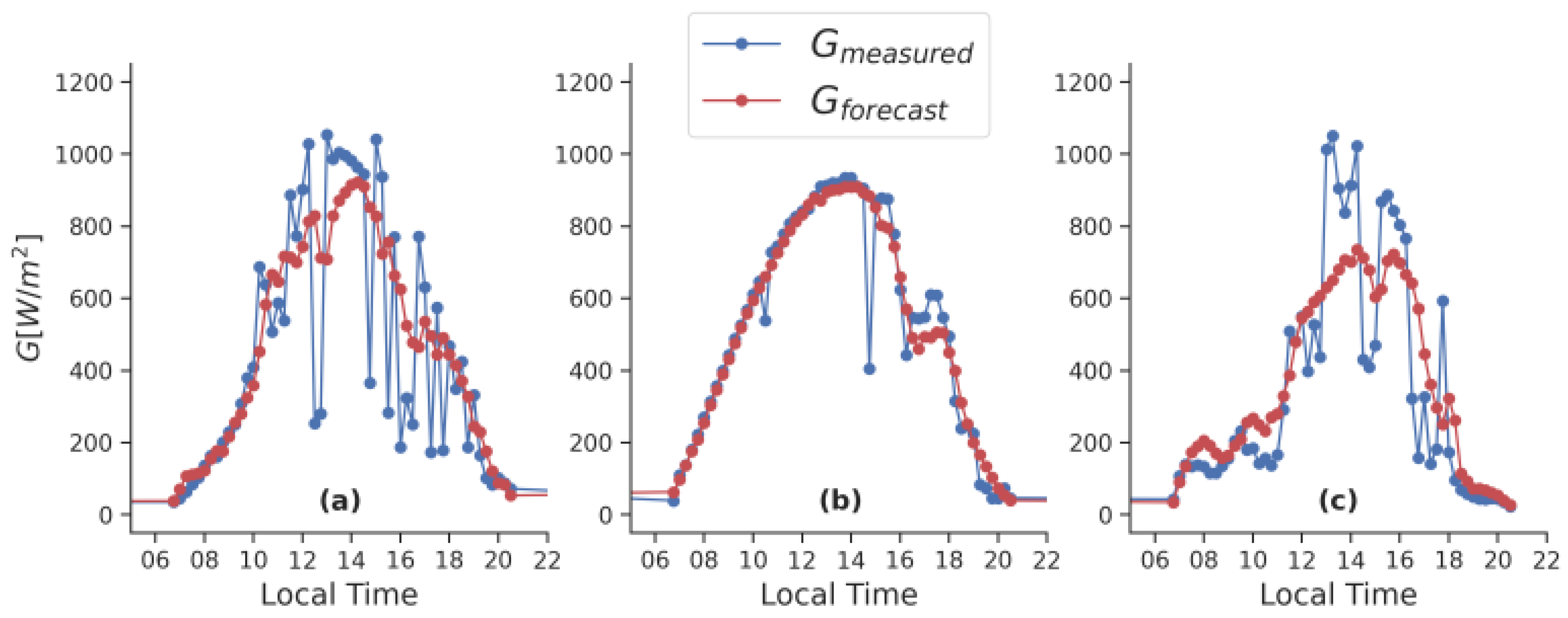
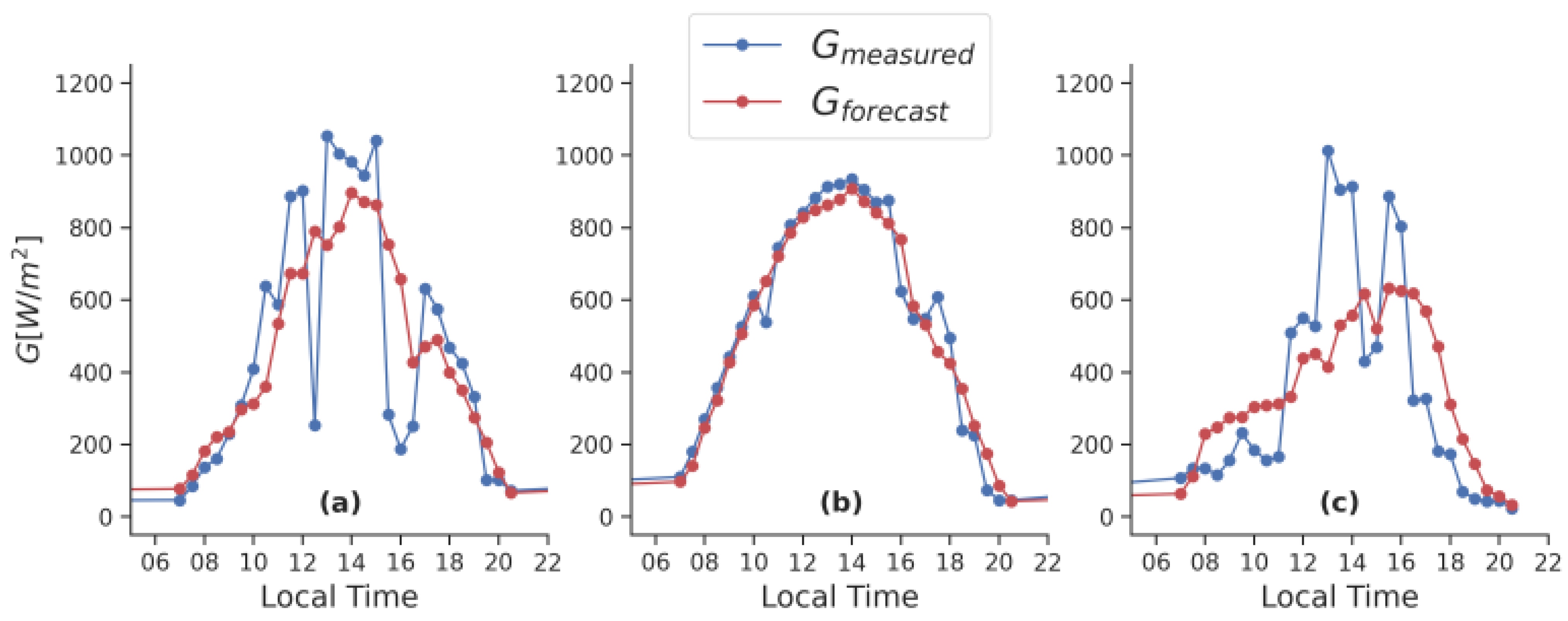
Figure 2, Figure 3 and Figure 4 compare the forecasts of the weighted ensemble ENw with measured data at various forecast horizons: 5 min (Figure 2), 15 min (Figure 3), and 30 min (Figure 4). For mostly clear sky periods, as showcased in Figure 2b, Figure 3b and Figure 4b, the ensemble performs very accurately. The forecasts almost perfectly overlap the measurements. During the same periods, ENw fails to forecast the magnitude of the sudden drops in measured solar irradiance caused by transient clouds. For the other days showcased, days with moderate to high variability in the state of the sky, ENw performs better at the shorter than the larger forecast horizons. Considering the 5-min forecast horizon, the curve given by the ensemble forecast follows the measurements with reasonable accuracy. ENw presents a low ability in capturing cloud enhancement phenomena in the high variable sky. At a 30 min forecast horizon (Figure 4), an adjustment of ENw to better capture the ramp in data is clearly necessary.
Table 1, Table 2, Table 3 and Table 4 present the performances of each individual model, as well as the ENm and ENw ensembles, compared to the baseline given by persistence. All models show an improvement in terms of skill score and nRMSE. There is only a small improvement in terms of MAPE. The statistical models (ARIMA and ES) achieve similar skill scores for all forecast horizons, with values between 3.8% and 5.8%. They do not introduce significant bias, with values of the nMBE close to zero.
The GBT model shows a significant improvement over the statistical models, with negligible differences in terms of bias or MAPE. GBT also shows consistent performance across all forecast horizons, with skill scores ranging from 8.5% to 13.9%, depending on the time horizon. The LSTM model outperforms each individual model by skill score for the shorter time horizons of 5 and 10 min; however, at larger time horizons, such as 30 min, it performs the worst out of all models. In our implementation, we have used higher granularity with data measured each minute one step ahead as input to the machine learning models. Future studies could research the impact of granularity on the performance of LSTM models for longer time horizons. LSTM models seem to introduce some positive bias, as showcased in Figure 1, as well.
The SI model performs remarkably well for forecast horizons longer than 10 min, especially for the 15-min forecast horizon, where a 17.2% skill score is achieved. However, for short forecast horizons, such as 5 min, its performance is lower than the performance of the statistical models. Because few changes in the state of the sky occur at such short time horizons, a larger lead time of 10 min was considered, only in this situation. For example, the inputs for the forecast given at moment t for the moment t + 1 are the sky images taken at moments t − 2, t − 1, and t. This applies only to the short time horizon of 5 min. The results presented in Table 1, Table 2, Table 3 and Table 4 show that, on this implementation, SI performs best at forecast horizons between 10 and 30 min. This confirms previous results with different implementations for the sky-imagery-based model.
Despite the contribution brought by the dynamics of the clouds in the sky, sometimes SI issues forecasts of poor quality. Figure 5 compares a good forecast (Figure 5a) with a poor one (Figure 5b). Forecasts are made at a 15-min forecast horizon based on two previous sky images taken 15 min apart. Both forecasts start from the same initial state of the sky, which is almost perfectly clear. On 26 May 2023 at 10:45 (Figure 5a), SI forecasts global solar irradiance of 755 W/m2, which is very close to the measured value of 745 W/m2. Differently, on 23 May 2023 at 12:45 (Figure 5b), SI forecasts global solar irradiance of 876 W/m2, while the measured value, 239 W/m2, is almost four times smaller. Visual inspection of Figure 5 shows that in both cases, the two sky photos, on which the forecasts are based, look very similar. The enormous difference between the accuracy of the forecasts is given by the local formation of clouds. The local formation and morphology of clouds is difficult to model even using information from the sky imager. Probably, in such a situation, an increase in data granularity may reduce the SI forecasts’ uncertainty.
Overall, when comparing the two proposed ensemble models (Table 1, Table 2, Table 3 and Table 4), a tradeoff is observed. Both show significantly increased performance in terms of nRMSE and skill score, with ENw being the best model. However, the tradeoff is observed in terms of nMBE and MAPE: the ENm ensemble performs better when considering these statistical indicators, at the cost of slightly lower skill scores.
5. Conclusions
The aim of this study was to increase the accuracy of intra-hour solar irradiance forecasts. A new ensemble approach, combining statistical extrapolation of time-series measurements with models based on machine learning and all-sky imagery, was proposed. The ensemble comprises five models: two classical statistics time series models (autoregressive integrated moving average (ARIMA) and exponential smoothing (ES)) two machine learning models (gradient boosted trees (GBT) and long short-term memory (LSTM)) and an all-sky imager-based method (SI).
The proposed ensemble approach demonstrated its effectiveness in intra-hour solar irradiance forecasting. The weighted average ensemble (ENw) exhibited the highest performance, yielding a skill score ranging from 15 to 20% for forecast horizons of 10 to 30 min. While the ensemble approach shows promising results, there is room for further enhancement. Future research will focus on increasing data granularity, particularly for LSTM and SI models, with the expectation of improved accuracy.
In conclusion, this study introduces a novel ensemble approach for intra-hour solar resource forecasting. The integration of statistical extrapolation, machine learning models, and all-sky imagery has demonstrated its potential in achieving accurate forecasts, with the ensemble ENw model showing the best performance.
Author Contributions
Conceptualization, S.-M.H., N.S. and M.P.; methodology, S.-M.H. and M.P.; software, S.-M.H.; formal analysis, S.-M.H., N.S. and M.P.; data curation, S.-M.H.; writing—original draft preparation, S.-M.H., N.S. and M.P.; writing—review and editing, N.S. All authors have read and agreed to the published version of the manuscript.
Funding
This work was supported by a grant of the Romanian National Authority for Scientific Research and Innovation, UEFISCDI project number PN-III-P2-2.1-PED-2021-0544.
Data Availability Statement
Data can be made available upon request.
Conflicts of Interest
The authors declare no conflict of interest.
Abbreviations
| ANN | Artificial Neural Network |
| ARIMA | Autoregressive integrated moving average |
| ES | Exponential smoothing |
| GBT | Gradient boosted decision trees |
| LSTM | Long short-term memory |
| MSE | Mean squared error |
| MAE | Mean absolute error |
| PCA | Principal component analysis |
| ET | Extremely randomized trees |
| RF | Random forest |
| nRMSE | Normalized root mean squared error |
| nMBE | Normalized mean bias error |
| MAPE | Mean absolute percentage error |
| SS | Skill score |
| PE | Persistence |
| Kt | Clearness index |
| SSN | Sunshine number |
| SI | Sky imagery |
| ENm | Ensemble based on the average of all models |
| ENw | Ensemble based on the weighted mean of all models |
| h | Solar elevation angle |
Appendix A. Statistical Measures of Accuracy
Let us consider n forecasted values, denoted , of the measured quantity mi. The following two statistical indicators (RMSE—root mean squared error, MAE—mean absolute error, and MBE—mean bias error) are commonly used to measure the forecasts accuracy:
To assess the performance of forecasting models operating on data with various magnitudes, normalized statistical indicators are employed (nRMSE—normalized root mean-squared error, nMBE—normalized mean bias error, and MAPE—mean absolute percentage error):
where represents the average of the measured values and defines the relative error for individual forecasts.
The skill score measures the relative improvement of a given model over a benchmark:
and are calculated with Equation (A1) and denote RMSE achieved by the tested and reference model, respectively. SS is often expressed as a percentage. Persistence is recommended as a reference in solar energy forecasting.
References
- Musiał, M.; Lichołai, L.; Katunský, D. Modern Thermal Energy Storage Systems Dedicated to Autonomous Buildings. Energies 2023, 16, 4442. [Google Scholar] [CrossRef]
- Blaga, R.; Paulescu, M. Quantifiers for the solar irradiance variability: A new perspective. Sol. Energy 2018, 174, 606–616. [Google Scholar] [CrossRef]
- Mills, A.; Ahlstrom, M.; Brower, M.; Ellis, A.; George, R.; Hoff, T.; Kroposki, B.; Lenox, C.; Miller, N.; Milligan, M.; et al. Dark shadows. Understanding variability and uncertainty of photovoltaics for integration with the electric power system. IEEE Power Energy 2011, 9, 33–41. [Google Scholar] [CrossRef]
- Sobri, S.; Koohi-Kamali, S.; Rahim, N.A. Solar photovoltaic generation forecasting methods: A review. Energy Convers. Manag. 2018, 156, 459–497. [Google Scholar] [CrossRef]
- Dileep, G. A survey on smart grid technologies and applications. Renew. Energy 2020, 146, 2589–2625. [Google Scholar] [CrossRef]
- Wai, R.-J.; Lai, P.-X. Design of Intelligent Solar PV Power Generation Forecasting Mechanism Combined with Weather Information under Lack of Real-Time Power Generation Data. Energies 2022, 15, 3838. [Google Scholar] [CrossRef]
- Tsai, W.-C.; Tu, C.-S.; Hong, C.-M.; Lin, W.-M. A Review of State-of-the-Art and Short-Term Forecasting Models for Solar PV Power Generation. Energies 2023, 16, 5436. [Google Scholar] [CrossRef]
- Blaga, R.; Sabadus, A.; Stefu, N.; Dughir, C.; Paulescu, M.; Badescu, V. A current perspective on the accuracy of incoming solar energy forecasting. Prog. Energy Combust. Sci. 2019, 70, 119–144. [Google Scholar] [CrossRef]
- Paulescu, M.; Paulescu, E. Short-term forecasting of solar irradiance. Renew. Energy 2019, 143, 985–994. [Google Scholar] [CrossRef]
- Gbémou, S.; Eynard, J.; Thil, S.; Guillot, E.; Grieu, S. A Comparative Study of Machine Learning-Based Methods for Global Horizontal Irradiance Forecasting. Energies 2021, 14, 3192. [Google Scholar] [CrossRef]
- Sawant, M.; Shende, M.K.; Feijóo-Lorenzo, A.E.; Bokde, N.D. The State-of-the-Art Progress in Cloud Detection, Identification, and Tracking Approaches: A Systematic Review. Energies 2021, 14, 8119. [Google Scholar] [CrossRef]
- Logothetis, S.-A.; Salamalikis, V.; Nouri, B.; Remund, J.; Zarzalejo, L.F.; Xie, Y.; Wilbert, S.; Ntavelis, E.; Nou, J.; Hendrikx, N.; et al. Solar Irradiance Ramp Forecasting Based on All-Sky Imagers. Energies 2022, 15, 6191. [Google Scholar] [CrossRef]
- Logothetis, S.-A.; Salamalikis, V.; Wilbert, S.; Remund, J.; Zarzalejo, L.F.; Xie, Y.; Nouri, B.; Ntavelis, E.; Nou, J.; Hendrikx, N.; et al. Benchmarking of solar irradiance nowcast performance derived from all-sky imagers. Renew. Energy 2022, 199, 246–261. [Google Scholar] [CrossRef]
- Rahimi, N.; Park, S.; Choi, W.; Oh, B.; Kim, S.; Cho, Y.-H.; Ahn, S.; Chong, C.; Kim, D.; Jin, C.; et al. A Comprehensive Review on Ensemble Solar Power Forecasting Algorithms. J. Electr. Eng. Technol. 2023, 18, 719–733. [Google Scholar] [CrossRef]
- Shan, S.; Li, C.; Ding, Z.; Wang, Y.; Zhang, K.; Wei, H. Ensemble learning based multi-modal intra-hour irradiance forecasting. Energy Convers. Manag. 2022, 270, 116206. [Google Scholar] [CrossRef]
- Box, G.E.P.; Jenkins, G.M.; Reinsel, G.C.; Ljung, G.M. Time series analysis. In Forecasting and Control, 5th ed.; Wiley: Hoboken, NJ, USA, 2016. [Google Scholar]
- Chen, T.; Guestrin, C. XGBoost: A Scalable Tree Boosting System. In Proceedings of the 22nd ACM SIGKDD International Conference on Knowledge Discovery and Data Mining, San Francisco, CA, USA, 13—17 August 2016; pp. 785–794. [Google Scholar]
- Persson, C.; Bacher, P.; Shiga, T.; Madsen, H. Multi-Site Solar Power Forecasting Using Gradient Boosted Regression Trees. Sol. Energy 2017, 150, 423–436. [Google Scholar] [CrossRef]
- Li, X.; Ma, L.; Chen, P.; Xu, H.; Xing, Q.; Yan, J.; Lu, S.; Fan, H.; Yang, L.; Cheng, Y. Probabilistic Solar Irradiance Fore-casting Based on XGBoost. Energy Rep. 2022, 8, 1087–1095. [Google Scholar] [CrossRef]
- Hochreiter, S.; Schmidhuber, J. Long Short-Term Memory. Neural Comput. 1997, 9, 1735–1780. [Google Scholar] [CrossRef]
- Liu, W.; Wang, Z.; Liu, X.; Zeng, N.; Liu, Y.; Alsaadi, F.E. A Survey of Deep Neural Network Architectures and Their Applications. Neurocomputing 2017, 234, 11–26. [Google Scholar] [CrossRef]
- Zang, H.; Cheng, L.; Ding, T.; Cheung, K.W.; Liang, Z.; Wei, Z.; Sun, G. Hybrid Method for Short-Term Photovoltaic Power Forecasting Based on Deep Convolutional Neural Network. IET Gener. Transm. Distrib. 2018, 12, 4557–4567. [Google Scholar] [CrossRef]
- Chu, Y.; Li, M.; Coimbra, C.F.M.; Feng, D.; Wang, H. Intra-Hour Irradiance Forecasting Techniques for Solar Power Integration: A Review. iScience 2021, 24, 103136. [Google Scholar] [CrossRef] [PubMed]
- Al-lahham, A.; Theeb, O.; Elalem, K.; A. Alshawi, T.; A.Alshebeili, S. Sky Imager-Based Forecast of Solar Irradiance Using Machine Learning. Electronics 2020, 9, 1700. [Google Scholar] [CrossRef]
- Jolliffe, I.T.; Cadima, J. Principal Component Analysis: A Review and Recent Developments. Philos. Trans. R. Soc. A Math. Phys. Eng. Sci. 2016, 374, 20150202. [Google Scholar] [CrossRef] [PubMed]
- Geurts, P.; Ernst, D.; Wehenkel, L. Extremely randomized trees. Mach. Learn. 2006, 63, 3–42. [Google Scholar] [CrossRef]
- Solar Platform of the West University of Timisoara. Available online: http://solar.physics.uvt.ro/srms (accessed on 5 August 2023).
- Liu, B.Y.; Jordan, R.C. The interrelationship and characteristic distribution of direct, diffuse and total solar radiation. Sol. Energy 1960, 4, 1–19. [Google Scholar] [CrossRef]
- Badescu, V.; Paulescu, M. Statistical properties of the sunshine number illustrated with measurements from Timisoara (Romania). Atmos. Res. 2011, 101, 194–204. [Google Scholar] [CrossRef]
- World Meteorological Organization. Guide to Meteorological Instruments and Methods of Observation. 2021. Available online: https://library.wmo.int/index.php?id=12407&lvl=notice_display (accessed on 5 August 2023).
Figure 1.
Illustration of models’ forecasts on 27 May 2023. Measured global solar irradiance is depicted on the background in blue.
Figure 1.
Illustration of models’ forecasts on 27 May 2023. Measured global solar irradiance is depicted on the background in blue.

Figure 2.
Measured and forecasted with the weighted average ensemble (ENw) solar irradiance for a forecast horizon of 5 min in 3 days from the test period: (a) 05/25, (b) 05/26, and (c) 05/27.
Figure 2.
Measured and forecasted with the weighted average ensemble (ENw) solar irradiance for a forecast horizon of 5 min in 3 days from the test period: (a) 05/25, (b) 05/26, and (c) 05/27.

Figure 3.
Measured and forecasted with the weighted average ensemble (ENw) solar irradiance for a forecast horizon of 15 min in 3 days from the test period: (a) 05/25, (b) 05/26, and (c) 05/27.
Figure 3.
Measured and forecasted with the weighted average ensemble (ENw) solar irradiance for a forecast horizon of 15 min in 3 days from the test period: (a) 05/25, (b) 05/26, and (c) 05/27.

Figure 4.
Measured and forecasted with the weighted average ensemble (ENw) solar irradiance for a forecast horizon of 30 min in 3 days from the test period: (a) 05/25, (b) 05/26, and (c) 05/27.
Figure 4.
Measured and forecasted with the weighted average ensemble (ENw) solar irradiance for a forecast horizon of 30 min in 3 days from the test period: (a) 05/25, (b) 05/26, and (c) 05/27.

Figure 5.
Fisheye photos of the sky taken at 15 min lag on (a) 26 May 2023 and (b) 23 May 2023.


Table 1.
Statistical indicators of accuracy for all models at a forecast horizon of 5 min.
| Model | nMBE | nRMSE | MAPE [%] | SS [%] |
|---|---|---|---|---|
| PE | 0.000 | 0.29 | 18.5 | - |
| ES | 0.000 | 0.279 | 20.6 | 3.8 |
| ARIMA | 0.000 | 0.277 | 20.0 | 4.4 |
| GBT | 0.002 | 0.265 | 26.4 | 8.5 |
| LSTM | 0.027 | 0.257 | 24.3 | 11.4 |
| SI | 0.045 | 0.287 | 35.2 | 1.1 |
| ENm | 0.015 | 0.255 | 24.1 | 12.1 |
| ENw | 0.023 | 0.255 | 26.6 | 11.9 |
Table 2.
Statistical indicators of accuracy for all models at a forecast horizon of 10 min.
| Model | nMBE | nRMSE | MAPE [%] | SS [%] |
|---|---|---|---|---|
| PE | 0.000 | 0.35 | 26.2 | - |
| ES | 0.002 | 0.333 | 28.8 | 4.9 |
| ARIMA | 0.001 | 0.331 | 28.2 | 5.4 |
| GBT | −0.007 | 0.308 | 34.8 | 11.9 |
| LSTM | 0.032 | 0.297 | 33.1 | 15 |
| SI | 0.059 | 0.305 | 37.3 | 12.9 |
| ENm | 0.017 | 0.294 | 30.6 | 15.9 |
| ENw | 0.047 | 0.292 | 35.0 | 16.4 |
Table 3.
Statistical indicators of accuracy for all models at a forecast horizon of 15 min.
| Model | nMBE | nRMSE | MAPE [%] | SS [%] |
|---|---|---|---|---|
| PE | 0.001 | 0.371 | 31.8 | - |
| ES | 0.003 | 0.352 | 34.9 | 5.3 |
| ARIMA | 0.003 | 0.35 | 33.7 | 5.8 |
| GBT | −0.003 | 0.319 | 37.4 | 13.9 |
| LSTM | −0.015 | 0.317 | 35.0 | 14.5 |
| SI | 0.055 | 0.307 | 40.6 | 17.2 |
| ENm | 0.008 | 0.306 | 33.8 | 17.8 |
| ENw | 0.032 | 0.298 | 38.1 | 19.8 |
Table 4.
Statistical indicators of accuracy for all models at a forecast horizon of 30 min.
| Model | nMBE | nRMSE | MAPE [%] | SS [%] |
|---|---|---|---|---|
| PE | 0.003 | 0.389 | 37.5 | - |
| ES | 0.007 | 0.369 | 40.8 | 5.4 |
| ARIMA | 0.007 | 0.368 | 40.3 | 5.1 |
| GBT | −0.018 | 0.337 | 42.1 | 13.5 |
| LSTM | −0.067 | 0.387 | 40.9 | 0.6 |
| SI | 0.060 | 0.353 | 49.7 | 9.2 |
| ENm | −0.002 | 0.326 | 40.1 | 16.3 |
| ENw | 0.017 | 0.324 | 44.4 | 16.8 |
Disclaimer/Publisher’s Note: The statements, opinions and data contained in all publications are solely those of the individual author(s) and contributor(s) and not of MDPI and/or the editor(s). MDPI and/or the editor(s) disclaim responsibility for any injury to people or property resulting from any ideas, methods, instructions or products referred to in the content. |
© 2023 by the authors. Licensee MDPI, Basel, Switzerland. This article is an open access article distributed under the terms and conditions of the Creative Commons Attribution (CC BY) license (https://creativecommons.org/licenses/by/4.0/).
Share and Cite
MDPI and ACS Style
Hategan, S.-M.; Stefu, N.; Paulescu, M. An Ensemble Approach for Intra-Hour Forecasting of Solar Resource. Energies 2023, 16, 6608. https://doi.org/10.3390/en16186608
AMA Style
Hategan S-M, Stefu N, Paulescu M. An Ensemble Approach for Intra-Hour Forecasting of Solar Resource. Energies. 2023; 16(18):6608. https://doi.org/10.3390/en16186608
Chicago/Turabian StyleHategan, Sergiu-Mihai, Nicoleta Stefu, and Marius Paulescu. 2023. "An Ensemble Approach for Intra-Hour Forecasting of Solar Resource" Energies 16, no. 18: 6608. https://doi.org/10.3390/en16186608
Note that from the first issue of 2016, this journal uses article numbers instead of page numbers. See further details here.