

Optimizing Lifespan of Circular Products: A Generic Dynamic Programming Approach for Energy-Using Products

1
Bosch Thermotechnology GmbH, Junkersstraße 20, 73249 Wernau (Neckar), Germany
2
Institute of Environmental Engineering, ETH Zurich, 8093 Zurich, Switzerland
3
Department of Energy Engineering, Sharif University of Technology, Tehran 1458889694, Iran
*
Author to whom correspondence should be addressed.
†
Current address: Robert Bosch GmbH, Robert-Bosch-Campus 1, 71272 Renningen, Germany.
Energies 2023, 16(18), 6711; https://doi.org/10.3390/en16186711
Submission received: 30 May 2023
/
Revised: 12 August 2023
/
Accepted: 14 August 2023
/
Published: 19 September 2023
(This article belongs to the Special Issue Pathways toward a Decarbonized Future Energy System: Sustainable Solutions)
Abstract
:Slowing down replacement cycles to reduce resource depletion and prevent waste generation is a promising path toward a circular economy (CE). However, an obligation to longevity only sometimes makes sense. It could sometimes even backfire if one focuses exclusively on material resource efficiency measures of the production phase and neglects implications on the use phase. The (environmental) lifespan of circular products should, therefore, be optimized, not maximized, considering all life cycle phases. In this paper, a generic method for determining the optimal environmental lifespan (OEL) of energy-using products (EuPs) in a CE is developed, allowing the simultaneous inclusion of various replacement options and lifetime extension processes, like re-manufacturing, in the assessment. A dynamic programming approach is used to minimize the cumulative environmental impact or costs over a specific time horizon, which allows considering an unordered sequence of replacement decisions with various sets of products. The method further accounts for technology improvement as well as efficiency degradation due to usage and a dynamic energy supply over the use phase. To illustrate the application, the OEL of gas heating appliances in Germany is calculated considering newly evolved products and re-manufactured products as replacement options. The case-study results show that with an average heat demand of a dwelling in Germany, the OEL is just 7 years for climate change impacts and 11 years for the aggregated environmental indicator, . If efficiency degradation during use is considered, the OEL for both environmental impact assessment methods even lowers to 1 year. Products are frequently replaced with re-manufactured products to completely restore efficiency at low investment cost, resulting in higher savings potential. This not only implies that an early replacement before the product breaks down is recommended but also that it is essential to maintain the system and, thus, to prevent potential efficiency degradation. The results for cost optimization, as well as currently observed lifespans, vary considerably from this.
1. Introduction
The concept of circular economy (CE) is experiencing increased attention [1] and has been integrated into the EU strategy to ensure sustainable consumption [2]. At the center of CE is the principle to close material cycles. Slowing down replacement cycles in order to use fewer products for the same service is another key principle of CE [3,4,5].
Slow cycles reduce the need for raw materials and, therefore, intend to protect the “environment’s capacity to provide natural resources of a useful quality” [6] for future generations. The value of materials embodied in products is, thus, preserved for as long as possible. This is considered superior to recycling by the waste hierarchy [7], as every recycling process step may lead to a degradation in material quality and the loss of its original functionality [8]. An example of this is the contamination of aluminum by copper that occurs during recycling [9,10] and reduces material properties, such as corrosion resistance. To restore the quality, one is forced to dilute the contaminants, which may result in additional environmental impacts and entropy production (both thermodynamic or statistical entropy [11]). Long-lasting products are, therefore, an important element of resource efficiency strategies [12], and the resulting prevention of generated waste shall secure the progress toward sustainable consumption [13]; while this statement is generally valid for products that do not cause any or, at least, only a small environmental impact during the use phase, prolonging the useful lifetime might not always be environmentally beneficial, even if it reduces the direct resource-related environmental burden from production [12,14,15]. For energy-using products (EuPs), such as washing machines or heating systems, the question arises whether greater environmental benefits are achieved by extending the life of the product or, on the contrary, by replacing the product early with a new, more energy-efficient model before it is broken [16,17]. A holistic assessment is pivotal to avoiding negative side effects and contributing to sustainable consumption. Together with Desing et al. [4], Allwood et al. [12] and Cooper and Gutowski [15], we conclude that the aim of CE should be to optimize the lifespan and not necessarily to maximize it.
Optimal Environmental Lifespan
The optimal environmental lifespan (OEL) of a product is the replacement time where the potential impact savings resulting from using a (more energy-efficient) replacement product are equal or higher than the embodied impacts of that product such that cumulative impacts over a time horizon become minimal. As the efficiency of products generally decreases with wear (e.g., on moving parts with dependence on load cycles) or with age (e.g., calcification in heat exchangers or deterioration of insulating properties of foam), it is necessary to consider not only the initial efficiency of the product and efficiency improvements of a potential replacement product but also efficiency degradation of the product in use [18]. Both, continuous technology change and efficiency degradation, tend to shorten the OEL.
Improved replacement times of EuPs have been studied a lot for energy-intensive products [19,20,21], especially for household appliances such as washing machines [22,23] or refrigerators [16,24,25,26]. To review them, the existing literature on the topic of replacement was found through a reverse search based on references in the review of Cooper and Gutowski [15], Schaubroeck et al. [27], Jensen et al. [28] and van Loon et al. [29] and expanded through a literature search in ScienceDirect. In general, there are two broad objectives for determining the OEL in the literature, which are listed in Table 1: either (a) by minimizing the impact rate at break-even or (b) by minimizing the cumulative impact over a time horizon. Concerning the first objective (a), most studies do not consider efficiency degradation and continuous technology change simultaneously. For example, Dewulf and Duflou [18] take only one of these into account at the same time, making the mathematical problem linear and analytically solvable. The same applies to approaches determining the eco-payback period, as discussed by van Nes and Cramer [14]. The alternative objective (b) of minimizing the cumulative impacts over a time horizon can also be numerically solved with mathematical series when neglecting various dynamics in the use phase [30]. Ardente and Mathieux [22] simplify the “environmental assessment of durability” even further by comparing exclusively certain scenarios with discrete efficiency improvements or fixed replacement times. This may limit the solution space so that only the better of the considered variants can be found but not the best possible variant or not the optimal solution. In contrast to this, if several dynamical effects are considered simultaneously, the optimization problem becomes mathematically non-linear and requires an optimization algorithm for a solution. The complexity of such an assessment has been demonstrated by Kim et al. [31] with a dynamic programming approach for automobiles [31] and refrigerators [32] in the U.S. Kim et al. [31] calculated the optimal usage duration of a product that minimizes total environmental impact over several product lifetimes with multiple possible replacements at an irregular frequency. Various other authors have applied their approach to further case studies [27], such as de Kleine et al. [33] and Bakker et al. [34]. Dynamic programming has been applied to many other product life cycle problems such as resource allocation. However, only one replacement option at a time with a predefined replacement order is considered. For example, Liu et al. [35] optimized an ordered replacement policy for residential lighting with a defined trajectory of different lighting technologies. Hence, investigating the best pathway with further relevant replacement options in a CE, such as re-use or re-manufacturing, is not possible simultaneously. Secondhand usage of products is, in general, not considered in the OEL literature. Studies addressing these options instead focus on a specific scope, e.g., under which conditions functioning devices collected at waste treatment plants shall be reconditioned for re-use or the embodied materials recycled [26,36].
What is missing is an approach assessing an unordered sequence of replacement decisions with various sets of products (e.g., first replace a product with a re-manufactured one, then switch to a new one and, finally, replace with a re-manufactured product again, or any other sequence) [27]. Such an approach should be capable of determining the OEL of EuPs at an irregular replacement frequency, taking into account various dynamics induced by CE measures.
In this paper, we develop a generic method for determining the OEL of products in a CE, based on Kim et al. [31], to consider various replacement options with re-manufacturing or a technology switch, which also allows considering a sequence of multiple, unordered replacements (Section 2). To illustrate the application, the OEL of gas heating appliances in Germany is calculated in a simplified case study (Section 3). Heating systems have only recently been included in the scope of legislations like the Waste of Electrical and Electronic Equipment (WEEE) Directive [38], which is why this product category is not as well documented as other EuPs. This paper will, therefore, enhance the state of knowledge not only by studying the OEL but also by presenting the current lifespan profile of heating systems and, moreover, by showing further novel data with an efficiency progression of the gas boiler technology (Section 3.1). The OEL results for climate change impacts and are compared to a conducted cost optimization (Section 4). Finally, OEL results are further discussed in an extended scenario analysis with different gas mixes of biomethane and green power to hydrogen.
2. Generic Lifespan Optimization of Circular Products
The OEL of EuPs is affected by various dynamics of opposing forces. On the one hand, it becomes shorter with a steep technological efficiency progression or efficiency degradation due to usage. On the other hand, higher manufacturing-related impacts (e.g., due to increased material use, making a product more durable), as well as reduced impacts due to improved energy infrastructure or sufficient/reduced (behavioral) use (e.g., decreasing frequency of use), extend the OEL. A generic dynamic programming approach is developed here to account for those dynamics in a CE during OEL assessment. The method is based on a combinatorial optimization problem in which all different replacement options in a CE can be represented with their respective impacts in a decision tree (Section 2.1). The aim is to find the optimal decision path in that tree that determines the optimal replacement schedule of a product when cumulative impacts become minimal (Section 2.2). This allows for determining the OEL, considering multiple possible replacements over the optimization horizon whose order is not predetermined. The general procedure is shown as a flowchart in Figure 1.
2.1. Developing Decision Tree with a Varying Number of Replacement Options
To determine the OEL of an EuP, the decision has to be modeled on whether to keep the old product (O1), which is then subject to efficiency degradation and may also require maintenance and repair, or to replace it with another product (O2, …, OΩ) at a given time. In the latter case, environmental impact is caused due to the production of that product as well as waste treatment and recycling of the old product. In any case, impacts arise from the energy requirements of product use. Such a decision can then be made again after a certain time step, . Repeating this decision process creates a decision tree with a number of possible paths of , whereby is the number of different decision options considered and N is the number of time steps, i.e., stages, considered over the optimization period . This is illustrated in Figure 2 for three decision options () and three stages ().
Considering more than just two decision options () allows for a more generic approach, in which the simultaneous inclusion of new (more efficient) products and CE principles, such as re-manufacturing, or even the assessment of the best time for a technology switch is possible. Describing such a mathematical optimization problem generically as a function of thereby extends the approach by Kim et al. [31]. This, first of all, requires defining the order of decision options (O1, O2, …, OΩ). As in the example before, the first option at each decision point is here defined to further use the product (O1). For all other options, the product is replaced at this point. Their order of decision options must remain the same at each decision point. What might change for these replacement options are, for example, the impact intensities for production and end of life (EoL), as well as the use phase. In this paper, replacement comprises circular strategies (e.g., re-manufacturing) as well as replacement with new products and technologies. Replacement is considered to happen with an equivalent product, not the same. On the other hand, repair and maintenance is something that takes place on-site, which is not considered a replacement strategy in our paper and, therefore, not depicted as an additional decision option but already included in Equation (3).
Next, a state j variable, which is the index for each pathway at stage k (time steps elapsed), must be defined to determine the position in the decision tree. This depends on the number of possible decision options, , and an option counter, o, that is iteratively increased between 1 and :
Since the first decision option is defined to continue using the product, no replacement occurs for any paths for which , and thus, the condition in Equation (2) holds.
2.1.1. Modeling Impacts in the Decision Tree
Then, the impact per time step (), or, in other words, the impact between two nodes, in Figure 2 can be described. It is a function of impacts from production (), recycling () and maintenance and repair (), as well as direct impacts stemming from product use itself (Equation (3)). Due to age, technology or stage specifics, they may all vary with stage, k, and state, j, which is represented with the corresponding indices in the individual formulas. For better understanding, Tables S2–S5 in Supplementary Materials (SM) provide all indices used to describe the functions necessary for the exemplary case from Figure 2.
No impacts from production as well as waste treatment and recycling need to be considered if the replacement condition from Equation (2) holds (see Equation (4)).
Impacts resulting directly from product use form the first part of the term in Equation (3) and are determined by the energy demand per time step, ; the technology as well as stage-dependent specific impact function, (e.g., per kWh input); and the efficiency of the product in use. The latter is determined with the initial efficiency of the product in use by if a replacement took place and by if the old product is further used (Equation (5)). It is then further reduced with the technology and age-dependent efficiency degradation function, . The age of the product in use, , is determined for this using Equation (6).
All products must be replaced at their maximum considered lifetime, (e.g., when existing at their maximum technical lifetime). In the generic approach, the impact at the tree elements where must be set to infinity (see Equation (7)), which results in a forced replacement by any of the given alternative options () in the optimization and implicitly eliminates the whole tree structure further down that path.
2.1.2. Technology-Specific Functions
For the functions determining efficiency degradation, ; the specific impact, ; and impact from maintenance and repair, , the same applies with respect to the indices as described for the product’s efficiency, (see Equation (5)). The degradation function, , is here defined to take values in the interval of , whereby a value of one means no degradation, and values smaller than one mean that the efficiency of the product degrades. The decline in efficiency is technology-specific and can, therefore, vary for each pathway in the decision tree. Any age-dependent function can be used to model the product-specific shape starting from an initial value of one (see Section 3). The same applies to impacts due to maintenance and repair, . This may depend on the age of the product and the technology as well. Accordingly, no impact from maintenance and repair may be considered in the first operational year of a product, i.e., after replacement.
To express technology improvements in efficiency over time, , and the progression of energy required per time step, , is also freely selectable by the modeler and, likewise, the functions for production, , and recycling, , impacts. Any discrete or continuous function, for example, starting from an initial value , , and (Equation (8)), can express this. What is necessary for this is to translate the elapsed time steps, k, into the elapsed time, t, with in the first place. In addition, the technology-specific functions have to be assigned to the corresponding indices (Equation (9)). In case only one technology is considered in an assessment, its functions may not depend on the pathway, j, so this assignment step may become obsolete.
2.2. Finding Optimal Path in the Decision Tree Determining Optimal Lifespan
The objective is to find the path in the decision tree with minimum cumulative environmental impact over the whole optimization period (), which implicitly determines the best replacement time. Therefore, all along one path must be summed up and the minimum of those sums according to Equation (10) selected (please note that the floor operator is used to define the corresponding index; this could be confused with absolute bars). This approach allows for considering multiple replacements over the optimization period. However, in the case of the last replacement, the product in use may have a remaining (technical) lifetime. To reduce the calculation complexity, the impacts from production and EoL are not adjusted to the temporal scope here [22].
2.2.1. Optimization of Cumulative Impacts with Dynamic Programming
To model all possible decision paths with their associated impacts is very computationally intense. This kind of problem can better be solved with a dynamic programming approach, which is based on Bellman’s optimality principle that an optimal solution to a problem is composed of optimal solutions to the sub-problems [39]. It is generally used to analyze sequential decision processes in order to find the optimal decision path that causes the best possible cumulative (environmental) costs [31]. For this purpose, the optimization problem is structured into multiple stages in order to solve only single-stage sub-problems at a time. These partial results are systematically stored and used in the next larger sub-problem. The optimization procedure is then recursively repeated until the overall N-stage optimum is found. In backward induction, problems are solved moving back, one stage at a time, until all stages are included and the global optimum is determined. The computation thereby starts at the final stage N of the problem. The objective function from Equation (10) can, therefore, be restructured as a recursive relationship with i as a counter for the node under consideration at stage k (Equation (11)). In this way, the minimum environmental impact over the current and subsequent stages, , is calculated by initializing the computation with as the so-called stage-zero problem. The last calculated stage is , which is the cumulative impact of the optimal path. The first replacement is considered to be possible after the first time step (), for example, after the first year ().
The impacts of the very first year as well as the production of the initial product have not yet been taken into account. They occur before the first decision, are, therefore, always the same for all options and, consequently, have no effect on the optimization result. They are added according to Equation (12) to determine the total minimum impacts, , from beginning to end.
2.2.2. Optimal Path
The dynamic programming result is the minimum cumulative impact at the optimization horizon, but the best replacement times are still unknown, even though the optimization result is an implicit consequence of them. Accordingly, the information of when to replace with which option, in other words, the definition of the optimal path in the decision tree, is still missing and, thus, also the lifespan of each individual product used. Which state the optimal path, , passes through at each stage, k, is obtained with forward calculation using Equation (13). The calculation thereby starts at stage 1, whereby minimum cumulative impacts, , at stage are known from the solved backward calculation (Equation (11)) this time. This result can then be used to calculate the impacts at each stage, , that lead to minimum cumulative impacts at the optimization horizon.
2.2.3. Optimal Lifespan
The optimal path, , in turn, determines the optimal lifespan, , of each product used, b, (numerator for the number of products) by iterating over Equation (14) until the replacement condition (Equation (2)) holds, with . The last product in the optimal path may well have a longer optimal lifespan than its age indicates at this point in time since its replacement will only pay off after the optimization horizon. Therefore, it is not taken into account in the calculation of the values.
In case no replacement is beneficial within the optimization horizon, T, OEL is defined to equal T as a baseline and should then be selected longer in the next assessment sequence. However, the last possible replacement always determines the path with minimum cumulative impacts for all previous replacements, which is why results will always depend on the selected optimization period due to the path dependencies of non-linear dynamics.
Life cycle cost (LCC) optimization works in a similar way; while discounting of impacts is not applied in the environmental assessment [40], it is taken into account in the economic assessment to consider the productivity of capital, for example. Possible subsidies that reduce the investment for a newly purchased product or pricing in of external costs, such as from climate damage, are also included. The focus of this paper is on environmental optimization, which is why the reader is referred to Supplementary Materials for necessary cost-related changes in the definition of time-step-specific impacts () (Supplementary Materials Section S2.1).
3. Application to Case Study
The installed heating stock in Germany is very old and accordingly very inefficient [41,42]. Gas boilers have the highest share of this () [43] and still represent the most sold heating systems for existing buildings [44]. Heating, thus, accounts for the largest part () of climate change impacts caused by households in Germany [45]. Hence, gas boilers should be replaced frequently to ensure that technological efficiency improvements diffuse into the market, reducing climate change impacts caused by households [46]. We, therefore, apply the generic method in a case study on residential heating systems in Germany. In the first step, simplifications are made for this illustration, such as the fact that only full substitutes for the gas boiler technology with newly evolved or re-manufactured products and, hence, no technology switch, for example, to heat pumps, is considered (, such that a decision tree, as illustrated in Figure 2, is created; O1: further use of the product; O2: newly evolved gas boiler; O3: re-manufactured gas boiler with restored initial efficiency of the respective product). The goal is to investigate the improvement potential of optimized replacement only within this product category. To illustrate its full potential, the effect of “green gas” is analyzed as well. We consider biomethane (produced from corn, etc.) and green power to hydrogen as green gases here. This discussion is particularly of interest where the technology switch, for example, to heat pumps, is technically limited by contextual dependencies of the housing, which is often still the case in Germany and in many other countries.
Life cycle assessment (LCA) is used to determine the required data on the potential environmental impacts of a product system. With LCA, the impacts on the environment caused by resource extraction or emissions are modeled for the entire life cycle [47]. The functional unit for the assessment is to satisfy the yearly heat demand of a German dwelling over the entire optimization period with a maximum of N boilers. In this context, a dwelling is an average residential unit that has all the rooms necessary for running a household and, consequently, has an average living space.
The OEL method is applied to two exemplary environmental impact assessment methods. Climate change as an essential core planetary boundary is beyond the safe operating space for sustainable human development [48,49] and is the most relevant impact category for EuPs using fossil-fuel-based energy carriers. In addition to this, the single score, , indicator is included in the assessment to take a holistic view. It is a single-score damage-oriented indicator that includes damages to human health, ecosystems and resource availability. Climate change impacts are calculated based on the IPCC [50] methodology (100-year time horizon) and based on Goedkoop et al. [51] methodology (H/A).
Moreover, we calculate the optimal lifespan for costs. Financial burdens are expressed with expenses only [52]. The prices always refer to the current prices of the respective first installation year.
The environmental inventory and impacts are modeled in Brightway 2 [53] with Ecoinvent (version 3.4 cut-off system model) as a background database [54]. Environmental impacts as well as cost data are then imported into the dynamic programming model in Matlab (R2017b).
3.1. Model Structure and Technology Assumptions for Gas Boilers
Gas boilers are replaced for various reasons [55]: reorganization due to other building projects, efficiency concerns, or the old product breaks down or is prone to breakdown. The design time of gas boilers is 15 years [56], which is chosen to be the optimization period here with a time step resolution () of 1 year, resulting in 14 decisions over time (). Therefore, using the product until the end of the design time is the baseline for comparing the impacts of the optimized replacement scenarios. Because the use phase of gas heating appliances comes with high environmental impacts, an optimization period of 15 years is sufficient to obtain stable OEL results. In contrast, the cost optimization requires an optimization period of 30 years with a time step resolution () of 2 years. The maximum considered lifespan of gas boilers () is assumed to be 30 years, which corresponds to the current legislative time limit under the German Energy Saving Act [57]. This means that has no influence on the OEL assessment in the case study.
The oldest boiler we assess here was initially installed in 2006 and reached its design time after 15 years in 2020. All other 15 recent installation years are also assessed as individual cases, whereby the time of initial installation defines the starting point and further course in the assumed technological efficiency progression. Moreover, the installation year defines the annual heat demand to cover (see Figure 3), as well as the electricity demand required for this. The latter is also linked to an annually differentiated, varying energy mix (dynamic energy system). In all 15 cases with different starting years (–), 3 maintenance schedules with different resulting efficiency degradation scenarios are assumed. The first scenario serves as a reference in which no efficiency degradation occurs () so that solely the influence of the technological efficiency progression is examined. In the second and third scenarios, efficiency degradation is assumed to represent either “annual and professional” (: , see Equation (15)) or “no, respectively, seldom” maintenance (: ).
3.1.1. Continuous Technology Improvement of Gas Boiler Technology
It is assumed that the gas boiler technology is mature today and has reached its technical limit, so after 2018, there will be no further efficiency improvements. Before this, gas boiler technology improved greatly. To determine the technological efficiency progression, , for this period, energy efficiency data of gas boilers from BMWI [58] are used. Parameters describing the general characteristics of the boiler are translated according to DIN 15316-4-1 [59] to derive the seasonal energy efficiency for space heating. This is supplemented with data from a German gas boiler producer for the most recent years [60]. A polynomial progression is fitted to the data for the most common rated capacity class of approximately 30 kW [61] without considering the production volume per gas boiler, taking into account the products that are available on the market for the end user (see Supplementary Materials Section S3.3.2).
3.1.2. Re-Manufacturing
Re-manufacturing is the process of restoring a used product to at least like-new condition [62], i.e., restoring the product to its initial efficiency. The de-installed product is brought back to the manufacturer (or a re-manufacturing service provider) where the so-called core (of the product) is reconditioned. Subsequently, the re-manufactured product is installed in replacement of another device for another customer, ensuring that the replacement is equivalent, although not identical, to the original product. During re-manufacturing, only the residual components and parts are replaced and, thus, recycled [63]. As a result, production-related resources are saved, and production costs are reduced. Therefore, production impacts can be assumed to be similar or even smaller than those caused by normal production [64,65], which may be expressed as a fraction of the impacts for a new product, .
To estimate the impact saving for re-manufacturing, we adapt the figures from Hummen and Wege [64], which analyze the re-manufacturing of a circulation pump used in gas boilers, to calculate the fraction, , of production impacts for a new boiler caused in re-manufacturing (see Supplementary Material Table S11). It is assumed that the initial efficiency of the core product is fully restored and that it is like new. The efficiency degradation curve is then assumed to be the same as for new products.
3.1.3. Efficiency Degradation
Efficiency degradation due to the use of gas boilers has various reasons. According to Baldi et al. [66] lime scaling in the heat cell (1 mm can cause a increase in energy demand for the same output), insulation degradation (which causes more heat loss) or actuator faults are the most important ones. Eleftheriadis and Hamdy [67] have shown that it is a significant factor to take into account in the energy performance assessment of buildings. They use degradation factors (F) for different maintenance schedules from Hendron [68] to express the efficiency decay over time, t, in order to evaluate the actual efficiency of the installed heating stock in the U.S. This rule of thumb is adapted with a Weibull function in the assessment here (Equation (15), see Supplementary Materials Section S3.3.4 for Weibull parameters , and , as well as degradation factors, F).
3.1.4. Heat Demand
In order to account for the increasing insulation standards of the building envelope and the following decrease in heat demand of buildings, the building stock in Germany is modeled considering various building typologies and specific refurbishment, as well as demolition rates [69,70]. Furthermore, specific heat demand per square meter and average living area per building class are used to derive an average heat demand per dwelling and year for Germany () (see Supplementary Materials Section S3.3.5 for the living-space- and insulation-dependent heat demand modeling). The derived average heat demand decreases by 21% between 2006 and 2020, meaning that a boiler from 2006 is not only less efficient than a boiler from 2020 but also has to cover a higher heat demand. It is assumed that no energetic renovation is conducted during the optimization period so that the heat demand remains constant at the level of the first installation year, , of the boiler (). The likely reduction in heat demand and its effect on per-case results is discussed in an extended scenario analysis in Section 3.3.
3.2. Further Assumptions for LCA and LCC
Inventory data for the LCA and LCC assessment are described in detail in Supplementary Materials Section S3.3.6. It is assumed that the material composition and weight as well as the production processes remain constant for all boilers over time; hence, the same environmental impact from production is always assumed. Similar to Baxter [65], we, thus, neglect any improvements in energy intensity in material production and assembly or any scaling relationships [71]. In contrast, production and installation are adjusted with the inflation rate for the assessment of financial burden. With regard to the environmental life cycle inventory, burden from EoL are taken into account with WEEE treatment. According to the chosen cut-off system model, these impacts are allocated to the waste producer. Further treatment of any valuable by-product is not included in line with the responsibility principle, as these impacts or credits will be allocated to the product in which the recycled materials are embodied. Further allocations that go beyond those from the selected cut-off system model are not taken into account when applying the method.
The share of natural gas and auxiliary electricity to produce 1 kWh of heat output is assumed to remain constant at and , respectively, over time for all gas boilers. It is, therefore, assumed that efficiency improvements are evenly distributed between the combustion process and the electrical components, which results in an overestimation of the efficiency development of the combustion process, as recent efficiency gains are rather achieved due to improved electrical components, such as the circulation pump. Moreover, no technology differentiation of the combustion technology itself is considered. The distinction between impacts caused by electricity use and natural gas consumption allows for the modeling of a dynamic electricity energy supply with varying energy mixes. Since the biggest environmental impact stems from the natural gas burned in the boiler (i.e., through consumption and combustion [72]), scenarios for an alternative fuel mix (see Section 3.3) seem most relevant.
Maintenance determines the efficiency degradation scenario in the model. It is assumed that a product that is not undergoing regular maintenance does not break earlier than a regularly maintained product but is subject to stronger efficiency degradation. Moreover, the impact of the repair itself, including necessary spare parts, is modeled with a Weibull function: the older the product is, the more repairs with more spare parts are necessary (see Supplementary Materials Section S3.2). Transport for maintenance and repair or replacement are included with specific transport distances in the environmental assessment, whereas they are already priced into the production or maintenance cost, respectively (see Supplementary Materials Section S3.3.6).
3.3. Extended Scenario Analysis
The OEL tends to be longer the smaller the impact intensities from the use phase become, which is why the impact of the use phase is reduced in extended scenario analysis for climate change impacts to better understand the results and to illustrate potential effects of an improved energy system. Biomethane and, especially, green power to hydrogen are repeatedly mentioned as important components on the road to a climate-neutral Germany [73]. However, biomethane is severely limited, for example, by the necessary land use required for food production, [74], and, therefore, has only lower importance as a characteristic transition technology for climate protection. The latter, on the other hand, is increasingly being discussed as an important lever in the course of the German hydrogen strategy [75]. Renewable energy (such as wind) is used to produce electricity for the electrolyzer to generate hydrogen, which is then injected into the natural gas pipeline and used as a mix in the heating boiler. Hydrogen in heating systems may have a high long-term potential and is currently technically limited to around in the gas mix by the boiler technology [76]. A changed gas mix with green power to hydrogen and biomethane as well as a reduced heat demand through improved insulation or better energy management is, therefore, assumed in an extended scenario analysis (see Supplementary Materials Section S3.3.7). Starting from the baseline scenario () from Section 3.1 (see Figure 4 for notation), the proportion of hydrogen and biomethane are first increased gradually in further scenarios (: green hydrogen, : with additional biomethane) and then heating further decarbonized with an additional reduced heat demand of (). These infrastructure scenarios are further combined with the efficiency degradation scenarios and cases for the initiation year, which are already used in the baseline scenarios (see scenario combination overview in Figure 4). The infrastructure scenarios remain constant per case, meaning that, for example, no gas mix switch is allowed within one scenario.
4. Results
The climate change impact optimization results for two selected extreme cases are shown in Figure 5. Each diagram illustrates the annual impacts for a scenario where the original boiler is used for 15 years compared to the optimized annual impacts. The peaks on the graph, represented by unfilled squares for re-manufactured products and filled circles for new products, show the impacts of production and recycling at each point of product replacement. In the first case, a gas boiler was initially installed in 2006 (). This boiler reaches its design time in 2020. The results show that it should have been optimally replaced 1 (), 7 () or even 14 times (), depending on the maintenance schedule (Figure 5a,c,e). This means that the OEL would be between 1 () and 7 years () in this case. If the boiler is replaced in line with this schedule, the environmental impact is up to 11% smaller than in a scenario in which the boiler is used for 15 years; while a replacement is only proposed with a new product when neglecting efficiency degradation, a mix of replacements with re-manufactured (O3) and new products (O2) is recommended by the optimization approach in the cases with efficiency degradation. In this way, some efficiency gains in the cohort of products are exploited, and such improvements are retained by re-manufacturing the respective product. The latter only results in tiny peaks in Figure 5 since impacts due to the re-manufacturing process are minor. The higher the efficiency degradation is, the more frequently re-manufacturing is recommended, even if more efficient products are available in the future. In contrast, if a boiler is installed for the first time in 2020 (), solely efficiency degradation influences the optimized replacement scheme, resulting in replacements with re-manufactured products every two years () or every year () as the OEL (Figure 5b,d,f). In this case, replacement with new products is of less advantage because the technology is already mature [64].
Cumulative climate change impacts in the baseline without optimization are significantly lower in than in . This is due to the improved boiler efficiency of and assumed heat demand reduction of . The gap even widens when efficiency degradation is also taken into account. Hence, it is important to keep boilers as maintained as possible, in particular, old boilers in older buildings. The higher the heat demand (e.g., poor insulation due to housing type), the shorter the optimal environmental lifespan becomes. However, an optimized replacement schedule can bring cumulative climate change impacts of all assessed cases closer together no matter how often and how well the boilers are maintained. This optimization result mainly depends on the maintenance scenario and less on the technological efficiency progression curve (i.e., the possible efficiency improvement).
The indicator for gas heating systems is less dominated by the use phase than in the case of climate change impacts. The distribution of the OEL results for the two environmental impact assessment methods are depicted as Tukey boxplots for all assessed cases () in Figure 6. For example, with no efficiency degradation (Figure 5b) is the outlier with an OEL of 15 years in Figure 6a for climate change impacts. The results are in the same order of magnitude as the previously selected extreme cases for climate change impacts in Figure 5. As a rule of thumb, the OEL of gas boilers is 7 years for climate change impacts and 11 years for if efficiency degradation is neglected. For an average heat demand, it is around 1 year for both environmental impact assessment methods if efficiency degradation is considered.
When it comes to life cycle cost optimization, replacement is only financially attractive for old, less efficient gas boilers within the optimization period of 30 years if efficiency degradation with “no or seldom maintenance” () is considered. The median lifespan is then at about 14 years and deviates accordingly by a power of 10 from the environmental assessment. In most cases, a break-even exists only after the chosen optimization horizon of 30 years. Even if damage from climate change impacts is priced in after 2020 according to the German fuel emissions trading act with 25 [77] or for all years with much higher cost estimates of from the German Environment Agency (UBA) [78], it still makes financially more sense for the end user to pay the price for the damage caused by the emitted greenhouse gases than to replace the appliance. The high production and installation costs do not pay off in the chosen optimization period, especially when future costs are discounted. However, the current dramatic price increase in 2022 is not included in the long-term gas price time series used, which could lead to earlier replacement in the other scenarios examined.
The OEL results differ significantly in regard to the investigated impact assessment methods and assumed maintenance schedules, as well as the shape of technological efficiency progression. Further detailed results are, therefore, presented in Supplementary Materials Section S3.4.
Extended Scenario Analysis
The OEL results show that the proportion of resulting impacts from the production phase to the use phase is decisive. This is the reason why results for climate change impacts and as well as costs vary considerably. The latter is also influenced by the discounting assumed. The results of the extended scenario analysis for climate change impacts are shown in Figure 7. It shows the reduction potential compared to normal usage with no replacement over 15 years and no improvement in the infrastructure. Each Tukey boxplot represents the reduction potential per evaluated scenario (, see Figure 4 for a scenario overview) of all 15 cases considered (: to ) with the respective maintenance plan. The assumed impact reduction potential due to improved infrastructure is arranged along the y-axis (, , and ) and the maintenance scenarios (, and ) are organized along the x-axis. The results from the baseline assessment can be found on the x-axis (). The climate change impact reduction potential of an optimized replacement schedule () decreases only a little with an improved infrastructure per maintenance scenario. It also has only little effect on the optimal lifespan. The scenario analysis shows accordingly that changed impacts from production due to different material composition and weight or different selected system boundaries for EoL would not drastically change the results. This could be of significance for other products, especially where a scaling relationship matters [71]. Similarly, system boundaries and methodological choices in LCA, e.g., the allocation method, could influence results there [79] as smaller impacts from production and EoL favor early replacement and vice versa.
The scenarios with no or seldom maintenance () have the highest reduction potential through optimized replacement. This is especially true when combining the replacement reduction potential with the infrastructure reduction potential. The combined total climate change impact reduction potential () is graphically represented as the third axis in Figure 7, a metric that is derived by adapting the approach by Thamling et al. [80] (see Supplementary Materials Section S3.3.7). Notably, is then, on average, above 31% for and above 23% for , again when compared to no change in infrastructure and normal usage over 15 years but with respective efficiency degradation. However, absolute impacts are, of course, much higher with efficiency degradation than without (see Figure S14), emphasizing the statement from before that newer boilers and housing standards are better than old ones. The same is true without improved infrastructure.
Both levers—improved infrastructure with reduced heat demand as well as decarbonized energy carriers and optimized replacement of gas boilers—are needed to minimize environmental impacts due to heating.
5. Discussion
5.1. Methodological Aspects
The developed generic method is an appropriate approach to analyze the optimal replacement schedule with multiple irregular replacements over the optimization horizon and, thus, to determine the optimal lifespan of circular products. It is possible to include all kinds of dynamic scenarios of efficiency development (technological improvements and degradation due to usage) as well as dynamic impacts over the entire optimization period (e.g., in production with circular economy measures such as re-manufacturing or energy supply as well as maintenance and repair) and still find the optimal global solution. This advantage is even more evident for cost optimization due to assumed necessary discounting. Other approaches may require strong simplifications or may require a numerical solution due to non-linearity, so the global optimum may not be found or path dependencies of future replacements may not be taken into account correctly, respectively, or not included at all. The introduced method allows for assessing the best decision pathway in a CE. Not only the comparison of one option to another at each point in time is then possible to consider and, thus, only a restricted solution space, but all replacement options at all decision points with their path dependencies. Hence, an unordered sequence of replacement decisions with various sets of products can be assessed.
For comparison, if only two replacement options are considered (; O1: keep old product; O2: replace with new evolved product) in alignment with the approach by Kim et al. [31], replacements are recommended less often and the savings potential is lower (see Supplementary Materials Section S3.5 and Table S29). For example, the average OEL is 2 years and the savings potential is for climate change impacts in case of moderate efficiency degradation (). In contrast, in the case study, any deterioration in efficiency was eliminated with fewer investment costs via re-manufacturing, resulting in shorter OEL and higher savings potential. This is particularly true when no efficiency gains can be additionally exploited across a cohort of products.
However, the generic formulation of the OEL method results in high computational needs. The number of possible decision paths is determined by , whereby is the number of different options considered each year and N is the number of time steps considered over the optimization period. It is still computational with a simple dynamic programming approach in a reasonable amount of time for two replacement options (). It is quite useful in analyzing decisions if the number of possible states (different replacement options in the tree) is not too large. Computational needs may be reduced with more sophisticated dynamic programming approaches. Although it is possible to reduce the computational efforts with fewer decision points (N) or longer time steps (), it is not recommended due to path dependencies. The latter results in higher uncertainties of the results. For example, with a time resolution of 1 year, a hypothetical “real” = 3.01 years would already yield in an = 4 years, meaning that the result range is . A higher time resolution, therefore, leads to a smaller OEL and, accordingly, also to a smaller necessary delta in efficiency. A shorter optimization period, on the other hand, can lead to the result that a replacement does not pay off within the considered time span. This problem applies, in particular, to the last possible replacement, which, however, determines the path with minimum cumulative impacts for all previous replacements. This could be mitigated by adjusting its impacts from production and EoL to the temporal scope, for example, by linearly allocating these impacts to the remaining lifetime and subtracting them similar to Ardente and Mathieux [22], which would decrease the total life cycle impacts from the last product. As without allocation, the OEL results would inevitably still remain strongly dependent on the optimization period.
Here, we chose an optimization period of 15 years, which is sufficient to obtain stable OEL results for environmental impacts in the case of heating systems due to their use phase intensity. In other cases, a more extended optimization period might be necessary, as in the case of cost optimization. A long optimization period is recommended in order to ensure that the results are stable and only slightly affected by it. This requires the collection of data for long time series, which may be subject to inherent uncertainties. This, in turn, requires the analysis of different scenarios based on sufficiently large variations in key parameters, such as by altering technological efficiency progression curves or efficiency degradation. For example, in this case study, it turns out that replacement makes sense more frequently with re-manufactured products for both environmental impact assessment methods with a stepped technological efficiency progression shape considering only the most efficient product. It simply takes longer until the next efficiency increase can be exploited so that re-manufacturing can eliminate any efficiency decrease in the meantime (see Supplementary Materials Section S3.4). Due to the mentioned small possible effects of efficiency improvements in this case study, the shape of the progression has only a minor influence on the specific OEL results here. However, a structured sensitivity study is only possible in terms of an extended scenario assessment with the generic method. Approaches like Monte Carlo simulation are not suitable due to the high computational needs. Accordingly, what is missing is a confidence interval for the OEL results that also reflects the inherent uncertainties of the LCA data used and of the assumed progression of, for example, efficiency degradation or technology improvement. For example, real-life efficiency could be smaller for condensing and smaller for conventional gas boilers [81] than assumed in this case study. In addition, the assumed efficiency degradation has to be treated with a certain tolerance range. This analysis clearly shows the necessity to better measure efficiency degradation during operations in order to be able to conduct more robust assessments. Real-time energy efficiency monitoring with connected boilers might enable this [66]. Measurements of energy efficiency losses by using chimney sweeps based on flue gas temperature could and should be used for general guidance for timely replacement and necessary maintenance with regard to the rule of thumb elaborated here. However, with their tolerances, they are not sufficient for the application here.
In this case study, the generic dynamic programming method is applied to three exemplary impact assessment methods, which lead to different results. The cost optimization results deviate considerably from the environmental assessment, as already shown in other studies, e.g., [31,64,82]. Environmental and financial impact dimensions should be aligned further possibly by pricing in all external effects and not only cost estimates for damages from climate change. In any case, should the OEL be determined for several impact assessment methods to give a holistic picture, the choice of which depends strongly on the product under investigation. Thus, in contrast to lifespan maximization, the objective, which shall be optimized, must be carefully chosen. Potential benefits in one impact category must be carefully weighted against other impact categories, which may lead to a Pareto front. Further impact categories may be resource depletion or exergy, which are sometimes stated as the minimization goal of CE, e.g., [4].
5.2. Case Study Implications
The OEL results for gas boilers are much smaller than for other products. For example, when considering two replacement options and neglecting the potential of re-manufacturing to eliminate efficiency degradation with low investment, the energy/CO results with efficiency degradation for automobiles are 8, 10 or 18 years, depending on the mileage driven per year in the U.S. [31]. The OEL of refrigerators is similarly long for without the consideration of degradation [25] and much shorter (2 to 11 years) for climate change impacts when degradation is considered [32]. These products have in common that they have significant use phase impacts, though not as much as gas boilers. The OEL results seem to be in the right range for gas boilers, suggesting that the current legislative time limit of 30 years under the German Energy Saving Act [57] is far too long. Such long time limits also contribute to the relatively long existing usage profile, with an average replacement time of 20 years in Germany (see Supplementary Materials Section S3.3.1 for corresponding analysis with data from the federation of German heating industry [83,84,85] and statistics of building construction work from Destatis [86]). Therefore, this study can serve as a benchmark for policymakers on how frequently gas heating appliances should be replaced.
In addition, this study can also be valuable for product designers, indicating that the design time of 15 years [56] is set far too long. A shorter design time would mean that less strict tolerances or materials with less strict requirements (for example, regarding the corrosion resistance of aluminum) can be used, potentially resulting in cheaper products and enabling earlier replacement. In the end, it could even enable the use of more secondary resources and, ultimately, support the transition toward a more circular economy. After all, materials may degrade during recycling processes through contamination and lose their purity, which leads to the deterioration of technical properties, such as corrosion resistance. However, the aim of reducing material requirements should not be misconstrued as a justification for deliberately designing products with a limited lifespan, a practice known as planned technical obsolescence, to stimulate continuous consumer demand for newer models [87]. Instead, the focus should be on avoiding over-engineering products, which eventually places more burden on the environment. This is not consistent with our general understanding of quality, as we tend to equate high-quality products with durability or with other functionalities, such as comfort, aesthetics or luxurious design. Quality could also be defined in terms of the environmental impact a product causes, in which case the minimum impact at OEL is considered as high quality. This means that replacement at the right time is not hindered and policies to improve the energy efficiency of products, such as the Ecodesign Directive [88], are promoted. To be able to implement such “quality” requirements already in the design phase requires a prospective OEL assessment with a presumed efficiency progression curve like it was conducted for in the case study here. One way to achieve this could be, for example, a systematic approach that combines patent analysis and environmental aspects [89] to determine what future developments might look like.
Users expect investment goods like heating systems to last long, especially when replacing them earlier is not financially attractive, and tend to slow replacements due to context dependencies [90]. They would likely not accept recommendations of shorter replacement intervals, neither with a new nor with a re-manufactured product. This social acceptability presumption makes it even more important to prioritize proper maintenance over optimal replacement [33] and install a high-efficiency product from the outset, which may be more expensive than a less efficient one but can reduce environmental impacts. To improve overall environmental performance while making it affordable at the same time, investment costs are already reduced with an updated funding policy of the Federal Office of Economics and Export Control (BAFA) in Germany. It increasingly aims to create incentives for faster market diffusion of renewable technologies [91] in order to make the best economic use of financial resources for decarbonizing heating. The amendment to the federal subsidy for efficient buildings (BEG) has also made it possible since 2021 to subsidize smart home systems to monitor and optimize use in order to reduce consumption [92]. Another lever for impact reduction is behavioral changes by the user. Contrary to the discussed technical measures of building renovation or boiler replacement, they do not require financial resources. A lower demand for comfort, for example, could lead to lower room temperatures or living space, which may still be sufficient for the user. This would oppose the historical trend, as a large part of the insulation efficiency gains has been eaten up by the increase in (per capita) living space [86]. Such a resulting lower heat demand then also leads to a longer optimal lifespan (compare, for example, and in Figure 5). Pérez-Belis et al. [36], for example, studied the behavioral use on recommendations for replacements of repaired vacuum cleaners in more detail.
Rational use of energy contributes strongly to environmental protection and climate change mitigation [50]. The most environmentally friendly use of energy is when energy is not needed at all or when it is used for the correct application where only minimum energy losses occur. Energy losses are generally measured in exergy or exergy destruction. In the case of heating systems, particularly those using fossil-fuel-based energy carriers, like gas boilers, most exergy destruction occurs during primary energy conversion and in the boiler itself [93]. Efficiency improvements of the boiler, thus, reduce exergy destruction. In addition, a lower heat demand due to good insulation, tight building envelopes and the use of passive gains directly results in less exergy destruction.
Maintaining a heating system and reversing possible unavoidable efficiency degradation (e.g., through lime scaling) by cleaning or replacing the causing components (e.g., the heat cell) is also essential to reduce energy loss. Re-manufacturing these components and upgrading them, if technically possible [12], to the best available technology could also reduce resource-related environmental impacts during production. With our case study, we specify that re-manufacturing is environmentally beneficial not only when the technology is mature [64,94] but, more precisely, if the efficiency progression of a cohort of products is only minor within a specific period. Therefore, the approach might support defining a time scale and efficiency progression range in which EuPs can be considered mature. However, we assumed that the initial efficiency of the product is completely restored during re-manufacturing, which might not always be the correct assumption [15]. If an efficiency drop is considered, results might alternate from our case study such that re-manufacturing shall be pursued less often.
The scope of this study is to assess the OEL of gas heating appliances to analyze the maximum environmental improvement potential of only this product category with maintenance and replacement. Just replacing the gas boiler with a more efficient boiler, whether it is a new one or a re-manufactured and upgraded one, could significantly hinder the switch to a low exergy heating technology [93] with better environmental performance, such as a heat pump, and, thus, severely limit the environmental improvement potential of heating. Heat pumps have a much better environmental performance than gas boilers when an electricity mix with high renewable share is used [95,96]. Including the technology switch to heat pumps in the assessment may, therefore, lead to a phase out of gas boilers and dramatically reduce the OEL of them. Examining this should, therefore, be the next step in the application of the generic dynamic programming method for heating systems, especially when contrasted with the more stringent use of green power to hydrogen. Only then, is it possible to study the best use of financial resources in order to minimize both the environmental and financial burden. In general, it is possible to include more than just two replacement options (), even if not yet conducted in the first application here; the method does allow it though.
6. Conclusions
The introduced generic dynamic programming method is suitable to analyze the overlapping effects of efficiency improvement and efficiency degradation simultaneously, as well as further dynamic impacts induced by CE measures or dynamic energy infrastructure; while a switch in overall technology to, for example, heat pumps was not considered in this case study to keep it simple, the method can also be used to accommodate for more disruptive scenarios. The strength of this method lies precisely in the multitude of possible dynamic scenarios that can be considered and allows several irregular, unordered replacements with circular measures over the optimization horizon. It is particularly useful for those products where the best CE pathway cannot be determined by a superficial analysis due to dynamic path dependencies and particularly where efficiency degradation has a big effect. The latter case concerns all kinds of EuPs, especially those with an (environmentally) significant use phase.
In order to improve the environmental performance of circular products in its entirety and to make an optimized replacement schedule affordable at the same time, innovative business models and further technical developments should enable an optimized replacement in a CE [97]. In practice, it requires clear communication of OEL results, as the recommendation of shorter lifetimes might contradict consumer perceptions that long-lifetime products are superior to short-lifetime ones.
This research, therefore, sets out that a lifespan indicator is important to develop (not only) for EuP. Simple longevity indicators measuring material circularity or resource efficiency [98,99] may provide misleading results because they fail to consider the interplay of various influencing factors. An LCA-based approach, as presented in this paper, is needed [100] to enhance CE metrics with a product-centric lifespan indicator [101]. Such a lifespan indicator could be based on the product-specific OEL [30] and allows for considering various alternative replacement options in a CE. It accounts for the waste of resources and unsustainable throughput of materials if a product is used shorter than its OEL. The same applies if a product is used for too long.
Only within the range of the derived OEL does it make sense to repair a broken product and to make spare parts available to avoid negative environmental side-effects from lifetime extension processes. This should be considered when implementing the “right to repair” in the EU [2]. An increased lifetime would delay the replacement with more energy-efficient alternatives. Even if this results in an increased waste volume, which then enters the recycling system, as of 2014, heating systems already accounted for about 10% of the collected waste of large household appliances in Germany [102]. This is expected to increase under the conditions discussed here.
Products should have a clearly defined lifetime and not be durable per se. Only optimized and not maximized lifespans can help ensure sustainable consumption and production patterns. This should be supported by optimal and predictive maintenance of a product to fully exploit the potential for improvement. The transition toward a sustainable circular economy, therefore, requires assessment methods, like the generic dynamic programming method, which can provide additional, and sometimes unexpected, insights and help to better understand a system in order to find optimal solutions. In some cases, the lifespan of circular EuPs might be reduced, not maximized, in a circular economy with measures such as re-manufacturing to eliminate unavoidable efficiency degradation. Such replacement policies can, thus, minimize cumulative impacts over several life cycles, even when new, more efficient products are available.
Supplementary Materials
The following are available online at https://www.mdpi.com/article/10.3390/en16186711/s1. They contain further information about used models with their implemented assumptions for input data, such as lifespan profile, heat demand, technological efficiency progression and degradation, as well as LCA and LCC inventory data. Moreover, detailed results are given on the level of each assessed case and as an overall summary per impact assessment method, including a comparison between two and three replacement options. Furthermore, a glossary for some definitions used in this paper is also given there. References [103,104,105,106,107,108,109,110,111,112,113,114,115,116,117,118,119,120,121,122,123,124,125,126,127] are cited in the Supplementary Materials.
Author Contributions
Conceptualization, T.H. and R.R.; methodology, T.H.; software, T.H.; validation, T.H.; formal analysis, T.H.; investigation, T.H.; writing—original draft preparation, T.H.; writing—review and editing, S.H. and R.R.; visualization, T.H.; supervision, S.H. All authors have read and agreed to the published version of the manuscript.
Funding
This research did not receive any specific grant from funding agencies in the public, commercial or not-for-profit sectors. T.H. receives financial support from Robert Bosch GmbH within the scope of a fixed-term employment contract for his PhD.
Data Availability Statement
Not applicable.
Acknowledgments
The authors would like to thank, in particular, Andreas Frömmelt and Friederike Neugebauer for valuable comments on this manuscript, as well as Markus Rotert and colleagues at Bosch Thermotechnology GmbH for the support and fruitful discussions on the topic; in particular, Philipp Perrin for the support on heat demand modeling and its historical trend; Michael Pittner for the data of historical boilers from BMWi; Philipp Wörner for discussing the allowed gas mixes in the heat cell; and Rainer Laun for support with historical sales data from BDH.
Conflicts of Interest
The authors declare that they have no known competing financial interests and declare herewith that there was no third-party influence on the research that could have appeared to influence the work reported in this paper.
Abbreviations
The following abbreviations are used in this manuscript:
| CE | Circular Economy |
| EoL | End of Life |
| EuP | Energy-Using Products |
| OEL | Optimal Environmental Lifespan |
| WEEE | Waste of Electrical and Electronic Equipment |
References
- Bocken, N.M.P.; Olivetti, E.A.; Cullen, J.M.; Potting, J.; Lifset, R. Taking the Circularity to the Next Level: A Special Issue on the Circular Economy. J. Ind. Ecol. 2017, 21, 476–482. [Google Scholar] [CrossRef]
- A New Circular Economy Action Plan: For a Cleaner and More Competitive Europe; European Commission: Brussels, Belgium, 2020.
- den Hollander, M.C.; Bakker, C.A.; Hultink, E.J. Product Design in a Circular Economy: Development of a Typology of Key Concepts and Terms. J. Ind. Ecol. 2017, 21, 517–525. [Google Scholar] [CrossRef]
- Desing, H.; Brunner, D.; Takacs, F.; Nahrath, S.; Frankenberger, K.; Hischier, R. A circular economy within the planetary boundaries: Towards a resource-based, systemic approach. Resour. Conserv. Recycl. 2020, 155, 104673. [Google Scholar] [CrossRef]
- Potting, J.; Hekkert, M.; Worrell, E.; Hanemaaijer, A. Circular Economy: Measuring Innovation in the Product Chain: Policy Report; Planbureau voor de Leefomgeving: The Hague, The Netherlands, 2017. [Google Scholar]
- Sonderegger, T.; Dewulf, J.; Fantke, P.; Souza, D.M.; Pfister, S.; Stoessel, F.; Verones, F.; Vieira, M.; Weidema, B.; Hellweg, S. Towards harmonizing natural resources as an area of protection in life cycle impact assessment. Int. J. Life Cycle Assess. 2017, 22, 1912–1927. [Google Scholar] [CrossRef]
- European Union. EU Waste Framework Directive: 2008/98/EC. Off. J. Eur. Union 2008, L 312, 3–30. [Google Scholar]
- Reuter, M.A.; van Schaik, A.; Gutzmer, J.; Bartie, N.; Abadías-Llamas, A. Challenges of the Circular Economy: A Material, Metallurgical, and Product Design Perspective. Annu. Rev. Mater. Res. 2019, 49, 253–274. [Google Scholar] [CrossRef]
- Castro, M.; Remmerswaal, J.; Reuter, M.A.; Boin, U. A thermodynamic approach to the compatibility of materials combinations for recycling. Resour. Conserv. Recycl. 2004, 43, 1–19. [Google Scholar] [CrossRef]
- Løvik, A.N.; Müller, D.B. A Material Flow Model for Impurity Accumulation in Beverage Can Recycling Systems. In Light Metals; Springer: Cham, Switzerland, 2014; pp. 907–911. [Google Scholar]
- Rechberger, H.; Graedel, T.E. The contemporary European copper cycle: Statistical entropy analysis. Ecol. Econ. 2002, 42, 59–72. [Google Scholar] [CrossRef]
- Allwood, J.M.; Ashby, M.F.; Gutowski, T.G.; Worrell, E. Material efficiency: A white paper. Resour. Conserv. Recycl. 2011, 55, 362–381. [Google Scholar] [CrossRef]
- Cooper, T. Slower Consumption Reflections on Product Life Spans and the “Throwaway Society”. J. Ind. Ecol. 2005, 9, 51–67. [Google Scholar] [CrossRef]
- van Nes, N.; Cramer, J. Product lifetime optimization: A challenging strategy towards more sustainable consumption patterns. J. Clean. Prod. 2006, 14, 1307–1318. [Google Scholar] [CrossRef]
- Cooper, D.R.; Gutowski, T.G. The Environmental Impacts of Reuse: A Review. J. Ind. Ecol. 2017, 21, 38–56. [Google Scholar] [CrossRef]
- Iraldo, F.; Facheris, C.; Nucci, B. Is product durability better for environment and for economic efficiency? A comparative assessment applying LCA and LCC to two energy-intensive products. J. Clean. Prod. 2017, 140, 1353–1364. [Google Scholar] [CrossRef]
- Ardente, F.; Talens Peiró, L.; Mathieux, F.; Polverini, D. Accounting for the environmental benefits of remanufactured products: Method and application. J. Clean. Prod. 2018, 198, 1545–1558. [Google Scholar] [CrossRef] [PubMed]
- Dewulf, W.; Duflou, J.R. The environmentally optimised lifetime: A crucial concept in life cycle engineering. In Proceedings of the Global Conference on Sustainable Product Development and Life Cycle Engineering, Berlin, Germany, 29 September–1 October 2004; pp. 59–62. [Google Scholar]
- Truttmann, N.; Rechberger, H. Contribution to resource conservation by reuse of electrical and electronic household appliances. Resour. Conserv. Recycl. 2006, 48, 249–262. [Google Scholar] [CrossRef]
- Bodlak, L. Ökologisch Optimale Lebensdauer von Weißware: Recherche zu Lebenszyklus-Studien (LCA) Ausgewählter Produktgruppen (Weißware); Energieinstitut Vorarlberg: Dornbirn, Austria, 2018. [Google Scholar]
- Guidance to Improve Product Durability; Wrap: Banbury, UK, 2019.
- Ardente, F.; Mathieux, F. Identification and assessment of product’s measures to improve resource efficiency: The case-study of an Energy using Product. J. Clean. Prod. 2014, 83, 126–141. [Google Scholar] [CrossRef]
- Gensch, C.O.; Blepp, M. Lebensdauer und Ersatzstrategien von Miele-Haushaltsgeräten; Öko-Institut e.V.: Freiburg, Germany, 2015. [Google Scholar]
- Boldoczki, S.; Thorenz, A.; Tuma, A. The environmental impacts of preparation for reuse: A case study of WEEE reuse in Germany. J. Clean. Prod. 2020, 252, 119736. [Google Scholar] [CrossRef]
- Bakker, C.; den Hollander, M.; van Hinte, E.; Zijlstra. Products That Last: Product Design for Circular Business Models; TU Delft Library: Delft, The Netherlands, 2014. [Google Scholar]
- Hischier, R.; Böni, H.W. Combining environmental and economic factors to evaluate the reuse of electrical and electronic equipment—A Swiss case study. Resour. Conserv. Recycl. 2021, 166, 105307. [Google Scholar] [CrossRef]
- Schaubroeck, S.; Schaubroeck, T.; Baustert, P.; Gibon, T.; Benetto, E. When to replace a product to decrease environmental impact? A consequential LCA framework and case study on car replacement. Int. J. Life Cycle Assess. 2020, 25, 1500–1521. [Google Scholar] [CrossRef]
- Jensen, P.B.; Laursen, L.N.; Haase, L.M. Barriers to product longevity: A review of business, product development and user perspectives. J. Clean. Prod. 2021, 313, 127951. [Google Scholar] [CrossRef]
- van Loon, P.; Diener, D.; Harris, S. Circular products and business models and environmental impact reductions: Current knowledge and knowledge gaps. J. Clean. Prod. 2021, 288, 125627. [Google Scholar] [CrossRef]
- Skelton, A.C.H.; Allwood, J.M. Product life trade-offs: What if products fail early? Environ. Sci. Technol. 2013, 47, 1719–1728. [Google Scholar] [CrossRef]
- Kim, H.C.; Keoleian, G.A.; Grande, D.E.; Bean, J.C. SI: Life cycle optimization of automobile replacement: Model and application: Dynamic Life Cycle Inventories for Mid-Sized Cars. Environ. Sci. Technol. 2003, 37, 5407–5413. [Google Scholar] [CrossRef] [PubMed]
- Kim, H.C.; Keoleian, G.A.; Horie, Y.A. Optimal household refrigerator replacement policy for life cycle energy, greenhouse gas emissions, and cost. Energy Policy 2006, 34, 2310–2323. [Google Scholar] [CrossRef]
- de Kleine, R.D.; Keoleian, G.A.; Kelly, J.C. Optimal replacement of residential air conditioning equipment to minimize energy, greenhouse gas emissions, and consumer cost in the US. Energy Policy 2011, 39, 3144–3153. [Google Scholar] [CrossRef]
- Bakker, C.; Wang, F.; Huisman, J.; den Hollander, M. Products that go round: Exploring product life extension through design. J. Clean. Prod. 2014, 69, 10–16. [Google Scholar] [CrossRef]
- Liu, L.; Keoleian, G.A.; Saitou, K. Replacement policy of residential lighting optimized for cost, energy, and greenhouse gas emissions. Environ. Res. Lett. 2017, 12, 114034. [Google Scholar] [CrossRef]
- Pérez-Belis, V.; Bakker, C.; Juan, P.; Bovea, M.D. Environmental performance of alternative end-of-life scenarios for electrical and electronic equipment: A case study for vacuum cleaners. J. Clean. Prod. 2017, 159, 158–170. [Google Scholar] [CrossRef]
- Chung, W.H.; Kremer, G.E.O.; Wysk, R.A. A dynamic programming method for product upgrade planning incorporating technology development and end-of-life decisions. J. Ind. Prod. Eng. 2017, 34, 30–41. [Google Scholar] [CrossRef]
- European Union. Commission Regulation (EU) No 622/2012 of 11 July 2012 amending Regulation (EC) No 641/2009 with regard to ecodesign requirements for glandless standalone circulators and glandless circulators integrated in productsText with EEA relevance. Off. J. Eur. Union 2012, L 180, 4–8. [Google Scholar]
- Bellman, R.E. Dynamic Programming; Princeton University Press: Princeton, NJ, USA, 1957. [Google Scholar]
- Hellweg, S.; Hofstetter, T.B.; Hungerbühler, K. Discounting and the Environment: Should Current Impacts be Weighted Differently than Impacts Harming Future Generations? Int. J. Life Cycle Assess. 2003, 8, 8–18. [Google Scholar] [CrossRef]
- EU Pathways to a Decarbonised Building Sector: How Replacing Inefficient Heating Systems Can Help Reach the EU Climate Ambitions; ECOFYS: Utrecht, The Netherlands, 2016.
- Effizienzklassen-Rechner; Bundesministerium für Wirtschaft und Klimaschutz (BMWI): Berlin, Germany, 2018.
- Der dena-Gebäudereport 2016: Statistiken und Analysen zur Energieeffizienz im Gebäudebestand; Deutsche Energie-Agentur (dena): Berlin, Germany, 2016.
- BRG. The European Heating Product Markets: Germany. 2018. Available online: https://www.brgbuildingsolutions.com (accessed on 21 January 2021).
- Energieverbrauch Privater Haushalte für Wohnen 2017 Erneut Gestiegen; DESTATIS: Wiesbaden, Germany, 2018.
- Oschatz, B.; Mailach, B. CO2-Einsparungen durch Heizungsmodernisierungen; BDH (Bundesverband der Deutschen Heizungsindustrie e.V.): Cologne, Germany, 2015. [Google Scholar]
- Hellweg, S.; Mila i Canals, L. Emerging approaches, challenges and opportunities in life cycle assessment. Science 2014, 344, 1109–1113. [Google Scholar] [CrossRef] [PubMed]
- Steffen, W.; Richardson, K.; Rockström, J.; Cornell, S.E.; Fetzer, I.; Bennett, E.M.; Biggs, R.; Carpenter, S.R.; de Vries, W.; de Wit, C.A.; et al. Sustainability. Planetary boundaries: Guiding human development on a changing planet. Science 2015, 347, 1259855. [Google Scholar] [CrossRef]
- The Global Risks Report 2020; World Economic Forum: Cologny, Switzerland, 2020.
- IPCC. Climate Change 2013: The Physical Science Basis. Working Group I Contribution to the Fifth Assessment Report of the Intergovernmental Panel on Climate Change; IPCC: Geneva, Switzerland, 2013. [Google Scholar]
- Goedkoop, M.; Heijungs, R.; Huijbregts, M.; de Schryver, A.; Struijs, J.; van Zelm, R. ReCiPe 2008: A Life Cycle Impact Assessment Method Which Comprises Harmonised Category Indicators at the Midpoint and the Endpoint Level. Report I: Characterisation; Ministerie van Volkshuisvesting Ruimtelijke Ordening en Milieubeheer: The Hauge, The Netherlands, 2013. [Google Scholar]
- Reich, M.C. Economic assessment of municipal waste management systems—Case studies using a combination of life cycle assessment (LCA) and life cycle costing (LCC). J. Clean. Prod. 2005, 13, 253–263. [Google Scholar] [CrossRef]
- Mutel, C. Brightway: An open source framework for Life Cycle Assessment. J. Open Source Softw. 2017, 2, 236. [Google Scholar] [CrossRef]
- Wernet, G.; Bauer, C.; Steubing, B.; Reinhard, J.; Moreno-Ruiz, E.; Weidema, B. The ecoinvent database version 3 (part I): Overview and methodology. Int. J. Life Cycle Assess. 2016, 21, 1218–1230. [Google Scholar] [CrossRef]
- Kemna, R.; Elburg, M.v.; Li, W.; Holsteijn, R.v. Preparation Study on Eco-design of Boilers: Task 3 Report: Consumer Behaviour & Local Infrastructure; European Commission: Brussels, Belgium, 2007. [Google Scholar]
- Toxopeus, M.E.; Haanstra, W.; van Gerrevink, M.R.; van der Meide, R. A Case Study on Industrial Collaboration to Close Material Loops for a Domestic Boiler. Procedia CIRP 2017, 61, 52–57. [Google Scholar] [CrossRef]
- Verordnung über Energiesparenden Wärmeschutz und Energiesparende Anlagentechnik bei Gebäuden (Energieeinsparverordnung—EnEV); Bundesanzeiger: Berlin, Germany, 2007.
- Energieeffizienz von Heizgeräten; BMWI: Berlin, Germany, 2018.
- DIN 15316-4-1:2017; Energetische Bewertung von Gebäuden—Verfahren zur Berechnung der Energieanforderungen und Nutzungsgrade der Anlagen: Wärmeerzeugung für die Raumheizung und Trinkwassererwärmung, Verbrennungssysteme (Heizungskessel, Biomasse), Modul M3-8-1, M8-8-1. Deutsches Institut für Normung: Berlin, Germany, 2017.
- Enterprise Resource Planning (ERP) Database at Bosch Thermotechnology GmbH; Bosch: Wetzlar, Germany, 2019.
- Kemna, R.; Elburg, M.v. Ecodesign Review Study: Task 2: Market Analysis. 2019. Available online: https://www.ecoboiler-review.eu/Boilers2017-2019/downloads/Boilers%20Task%202%20final%20report%20July%202019.pdf (accessed on 29 May 2023).
- BSI 8887-2:2009; Design for Manufacture, Assembly, Disassembly and End-of-life Processing (MADE). Terms and Definitions. British Standards Institution: London, UK, 2009.
- Nasr, N.; Russell, J.; Bringezu, S.; Hellweg, S.; Hilton, B.; Kreiss, C.; von Gries, N. Re-defining Value: The Manufacturing Revolution: Remanufacturing, Refurbishment, Repair and Direct Reuse in the Circular Economy: A Report of the International Resource Panel; International Resource Panel: Paris, France, 2018. [Google Scholar]
- Hummen, T.; Wege, E. Remanufacturing of Energy using Products makes sense only when technology is mature: Introducing a Circular Economy indicator for remanufacturing based on a parameterized LCA and LCC assessment of a circulation pump. In Progress in Life Cycle Assessment 2019; Albrecht, S., Fischer, M., Leistner, P., Schebek, L., Eds.; Springer: Cham, Switzerland, 2020; pp. 67–82. [Google Scholar]
- Baxter, J. Systematic environmental assessment of end-of-life pathways for domestic refrigerators. J. Clean. Prod. 2019, 208, 612–620. [Google Scholar] [CrossRef]
- Baldi, S.; Le Quang, T.; Holub, O.; Endel, P. Real-time monitoring energy efficiency and performance degradation of condensing boilers. Energy Convers. Manag. 2017, 136, 329–339. [Google Scholar] [CrossRef]
- Eleftheriadis, G.; Hamdy, M. The Impact of Insulation and HVAC Degradation on Overall Building Energy Performance: A Case Study. Buildings 2018, 8, 23. [Google Scholar] [CrossRef]
- Hendron, R. Building America Performance Analysis Procedures for Existing Homes; National Renewable Energy Laboratory: Golden, CO, USA, 2006. [Google Scholar] [CrossRef]
- Enerdata. Entranze Forecasts Database. 2014. Available online: https://entranze-scenario.enerdata.net/site/ (accessed on 14 August 2017).
- Diefenbach, N. Deutscher Gebäudebestand: Basisdaten und Modellrechnungen bis 2020; Institut Wohnen und Umwelt GmbH: Darmstadt, Germany, 2010. [Google Scholar]
- Caduff, M.; Huijbregts, M.A.; Koehler, A.; Althaus, H.J.; Hellweg, S. Scaling Relationships in Life Cycle Assessment. J. Ind. Ecol. 2014, 18, 393–406. [Google Scholar] [CrossRef]
- Vignali, G. Environmental assessment of domestic boilers: A comparison of condensing and traditional technology using life cycle assessment methodology. J. Clean. Prod. 2017, 142, 2493–2508. [Google Scholar] [CrossRef]
- BDEW. Wie Heizt Deutschland 2019? BDEW: Berlin, Germany, 2019. [Google Scholar]
- BMU. Klimaschutzplan 2050: Klimaschutzpolitische Grundsätze und Ziele der Bundesregierung; BMU: Berlin, Germany, 2016. [Google Scholar]
- BMWI. Nationales Reformprogramm 2020—Die Nationale Wasserstoffstrategie; BMWI: Berlin, Germany, 2020. [Google Scholar]
- Marcogaz. Overview of Available Test Results and Regulatory Limits Forhydrogen Admission into Existing Natural Gas Infrastructure and End Use; Marcogaz: Brussels, Belgium, 2019. [Google Scholar]
- BMUB. Entwurf eines Ersten Gesetzes zur Änderung des Brennstoffemissionshandelsgesetzes; BMUB: Berlin, Germany, 2020. [Google Scholar]
- Bünger, B.; Matthey, A. Methodenkonvention 3.0 zur Ermittlung von Umweltkosten: Methodische Grundlagen; Umwelt Bundesamt: Dessau-Roßlau, Germany, 2018. [Google Scholar]
- Hauschild, M.Z.; Rosenbaum, R.K.; Olsen, S.I. (Eds.) Life Cycle Assessment: Theory and Practice; Springer: Cham, Switzerland, 2017. [Google Scholar]
- Thamling, N.; Pehnt, M.; Kirchner, J. Hintergrundpapier zur Energieeffizienzstrategie Gebäude: Erstellt im Rahmen der Wissenschaftlichen Begleitforschung zur ESG; Prognos: Basel, Switzerland, 2015. [Google Scholar]
- Kemna, R.; Elburg, M.V.; van den Boorn, R.; Aarts, S. Ecodesign Review Study: Task 5: Environment and Economics; European Commission: Brussels, Belgium, 2019. [Google Scholar]
- Bobba, S.; Ardente, F.; Mathieux, F. Environmental and economic assessment of durability of energy-using products: Method and application to a case-study vacuum cleaner. J. Clean. Prod. 2016, 137, 762–776. [Google Scholar] [CrossRef]
- BDH. Heizungsmarkt Deutschland; BDH: Köln, Germany, 2012. [Google Scholar]
- BDH. Marktentwicklung Wärmeerzeuger 2005–2015; BDH: Köln, Germany, 2015. [Google Scholar]
- BDH. Wärmewende: Keine Energiewende ohne den Wärmemarkt; BDH: Köln, Germany, 2019. [Google Scholar]
- Destatis. Statistik der Baufertigstellungen; DESTATIS: Wiesbaden, Germany, 2019. [Google Scholar]
- Jacob, P. Projected Obsolescence in Electric and Electronic Consumer Equipment? What are the Limiters of Lifetime, Service Life and Repairability of Modern Consumer Electr(on)ics? In Proceedings of the Electronics Goes Green 2020+, Online, 1 September 2020.
- European Union. Directive 2009/125/EG of the European Parliament and of the Council of 21 October 2009: Establishing a framework for the setting of ecodesign requirements for energy-related products. Off. J. Eur. Union 2009, L 285, 10–35. [Google Scholar]
- Spreafico, C.; Landi, D.; Russo, D. A new method of patent analysis to support prospective life cycle assessment of eco-design solutions. Sustain. Prod. Consum. 2023, 38, 241–251. [Google Scholar] [CrossRef]
- Wesche, J.P.; Negro, S.O.; Dütschke, E.; Raven, R.; Hekkert, M.P. Configurational innovation systems—Explaining the slow German heat transition. Energy Res. Soc. Sci. 2019, 52, 99–113. [Google Scholar] [CrossRef]
- Bafa. Förderübersicht: Heizen mit Erneuerbaren Energien 2020; BAFA: Eschborn, Germany, 2020. [Google Scholar]
- Bafa. Förderübersicht: Bundesförderung für Effiziente Gebäude (BEG); BAFA: Eschborn, Germany, 2021. [Google Scholar]
- Schmidt, D.; Shukuya, M. New ways towards increased efficiency in the utilization of energy flows in buildings. In Proceedings of the Second International Building Physics Conference, Leuven, Belgium, 14–18 September 2003; pp. 671–681. [Google Scholar]
- Gutowski, T.G.; Sahni, S.; Boustani, A.; Graves, S.C. Remanufacturing and energy savings. Environ. Sci. Technol. 2011, 45, 4540–4547. [Google Scholar] [CrossRef]
- Tolga Balta, M.; Kalinci, Y.; Hepbasli, A. Evaluating a low exergy heating system from the power plant through the heat pump to the building envelope. Energy Build. 2008, 40, 1799–1804. [Google Scholar] [CrossRef]
- Abusoglu, A.; Sedeeq, M.S. Comparative exergoenvironmental analysis and assessment of various residential heating systems. Energy Build. 2013, 62, 268–277. [Google Scholar] [CrossRef]
- Becker-Hardt, D. Development and Evaluation of Circular Business Models in the Market of Residential Heating: Analysis of Needed Design Implications. Master’s Thesis, University of Kassel, Kassel, Germany, 2018. [Google Scholar]
- Towards the Circular Economy; Ellen Mc Arthur Foundation: Isle of Wight, UK, 2015.
- Franklin-Johnson, E.; Figge, F.; Canning, L. Resource duration as a managerial indicator for Circular Economy performance. J. Clean. Prod. 2016, 133, 589–598. [Google Scholar] [CrossRef]
- Elia, V.; Gnoni, M.G.; Tornese, F. Measuring circular economy strategies through index methods: A critical analysis. J. Clean. Prod. 2017, 142, 2741–2751. [Google Scholar] [CrossRef]
- Parchomenko, A.; Nelen, D.; Gillabel, J.; Rechberger, H. Measuring the circular economy—A Multiple Correspondence Analysis of 63 metrics. J. Clean. Prod. 2019, 210, 200–216. [Google Scholar] [CrossRef]
- Waste Electrical and Electronic Equipment (WEEE) by Waste Management Operations; Eurostat: Luxembourg, 2019.
- prEN 45550:2018; Definitions Related to Material Efficiency. CEN/CLC: Brussels, Belgium, 2018.
- Wang, F.; Huisman, J.; Stevels, A.; Baldé, C.P. Enhancing e-waste estimates: Improving data quality by multivariate Input-Output Analysis. Waste Manag. 2013, 33, 2397–2407. [Google Scholar] [CrossRef] [PubMed]
- Thiébaud-Müller, E.; Hilty, L.M.; Schluep, M.; Widmer, R.; Faulstich, M. Service Lifetime, Storage Time, and Disposal Pathways of Electronic Equipment: A Swiss Case Study. J. Ind. Ecol. 2018, 22, 196–208. [Google Scholar] [CrossRef]
- Erhebungen des Schornsteinfegerhandwerks für 2013; ZIV: Sankt Augustin, Germany, 2013.
- Gas Kann Grün: Die Potentiale von Biogas/Biomethan: Status Quo, Fakten und Entwicklung; BDEW: Berlin, Germany, 2019.
- Adolf, J.; Schabla, U.; Lücke, A.; Breitenbach, L.; Bräuninger, M.; Leschus, L.; Ehrlich, L.; Otto, A.H.; Oschatz, B.; Mailach, B. Shell BDH Hauswärme-Studie: Klimaschutz im Wohnungssektor—Wie Heizen wir morgen? Fakten, Trends und Perspektiven für Heiztechniken bis 2030; Hamburgische WeltWirtschaftsInstitut: Hamburg, Germany, 2013. [Google Scholar]
- Baehr, H.D. Thermodynamik des Heizens und Kühlens. In Thermodynamik; Baehr, H.D., Ed.; Springer: Berlin/Heidelberg, Germany, 2002; pp. 556–593. [Google Scholar]
- European Union. Council Directive 92/42/EEC of 21 May 1992 on efficeincy requirements for new hot-water boilers fired with liquid or gaseous fuels. Off. J. Eur. Union 1992, L 167, 17–28. [Google Scholar]
- Holsteijn, R.v.; Kemna, R.; Elburg, M.v.; Wierda, L. Ecodesign Review Study: Task 7: Scenarios; European Commission: Brussels, Belgium, 2019. [Google Scholar]
- Energieeffizienzstrategie Gebäude: Wege zu einem Nahezu Klimaneutralen Gebäudebestand; BMWI: Berlin, Germany, 2015.
- Diefenbach, N.; Clausnitzer, K.D. Datenbasis Gebäudebestand: Datenerhebung zur Energetischen Qualität und zu den Modernisierungstrends im Deutschen Wohngebäudebestand; Institut Wohnen und Umwelt: Darmstadt, Germany; Bremer Energie-Institut: Bremen, Germany, 2010. [Google Scholar]
- Klimaschutz im Wohngebäudebereich: Wie Können Wir die Klimaschutzziele im Bereich der Wohngebäude in Deutschland bis 2050 Erreichen? nymoen: Berlin, Germany, 2017.
- Entranze: Policies to ENforce the TRAnsition to Nearly Zero Energy Buildings in the EU-27; Enerdata: Grenoble, France, 2014.
- Substitutionsquote: Ein Realistischer Erfolgsmaßstab für die Kreislaufwirtschaft; Umwelt Bundesamt: Dessau-Roßlau, Germany, 2019.
- Entwicklung der Energiemärkte—Energiereferenzprognose; Prognos: Basel, Switzerland, 2014.
- Gasheizung: Kosten und Preise für Ihre Heizung Berechnen; Bosch: Wetzlar, Germany, 2016.
- Verbraucherpreisindex für Deutschland: (Tabellen ab 1948); DESTATIS: Wiesbaden, Germany, 2020.
- Herausforderungen an die Deutsche Wettbewerbsfähigkeit durch einen Neuen Weltenergiemarkt; IHS: Berlin, Germany, 2013.
- Verivox-Verbraucherpreisindex: Gaspreis für Privathaushalte in Deutschland bei einem Gasverbrauch von 20.000 kWh in den Jahren 2005 bis 2020; Verivox: Heidelberg, Germany, 2020.
- Hummen, T. Recycling of Boilers: Material Value of a Gas Boiler and Circulation Pump. Personal communication with Markus Hutzler from Alba. 2019.
- Naturstrom Biogas | 100% Erneuerbare Energien von NATURSTROM; Naturstrom: Düsseldorf, Germany, 2020.
- Anwendungsbilanzen zur Energiebilanz Deutschland: Endenergieverbrauch nach Energieträgern und Anwendungszwecken; AG Energiebilanzen e.V.: Berlin, Germany, 2019.
- Zhang, X.; Bauer, C.; Mutel, C.L.; Volkart, K. Life Cycle Assessment of Power-to-Gas: Approaches, system variations and their environmental implications. Appl. Energy 2017, 190, 326–338. [Google Scholar] [CrossRef]
- Emissionsbilanz Erneuerbarer Energieträger: Bestimmung der Vermiedenen Emissionen im Jahr 2012; Umwelt Bundesamt: Dessau-Roßlau, Germany, 2013.
- Kemna, R.; Elburg, M.v. Ecodesign Review Study: Task 3: Space and Water Heating Demand and Usage. 2019. [Google Scholar]
Figure 1.
Flowchart showing how, in the proposed framework, the decision tree is developed using inputs to determine the environmental impacts in the decision tree (modeling), and then, the cumulative impacts are optimized over the entire optimization horizon using a dynamic programming approach to determine the optimal lifespan of each product used (optimization).
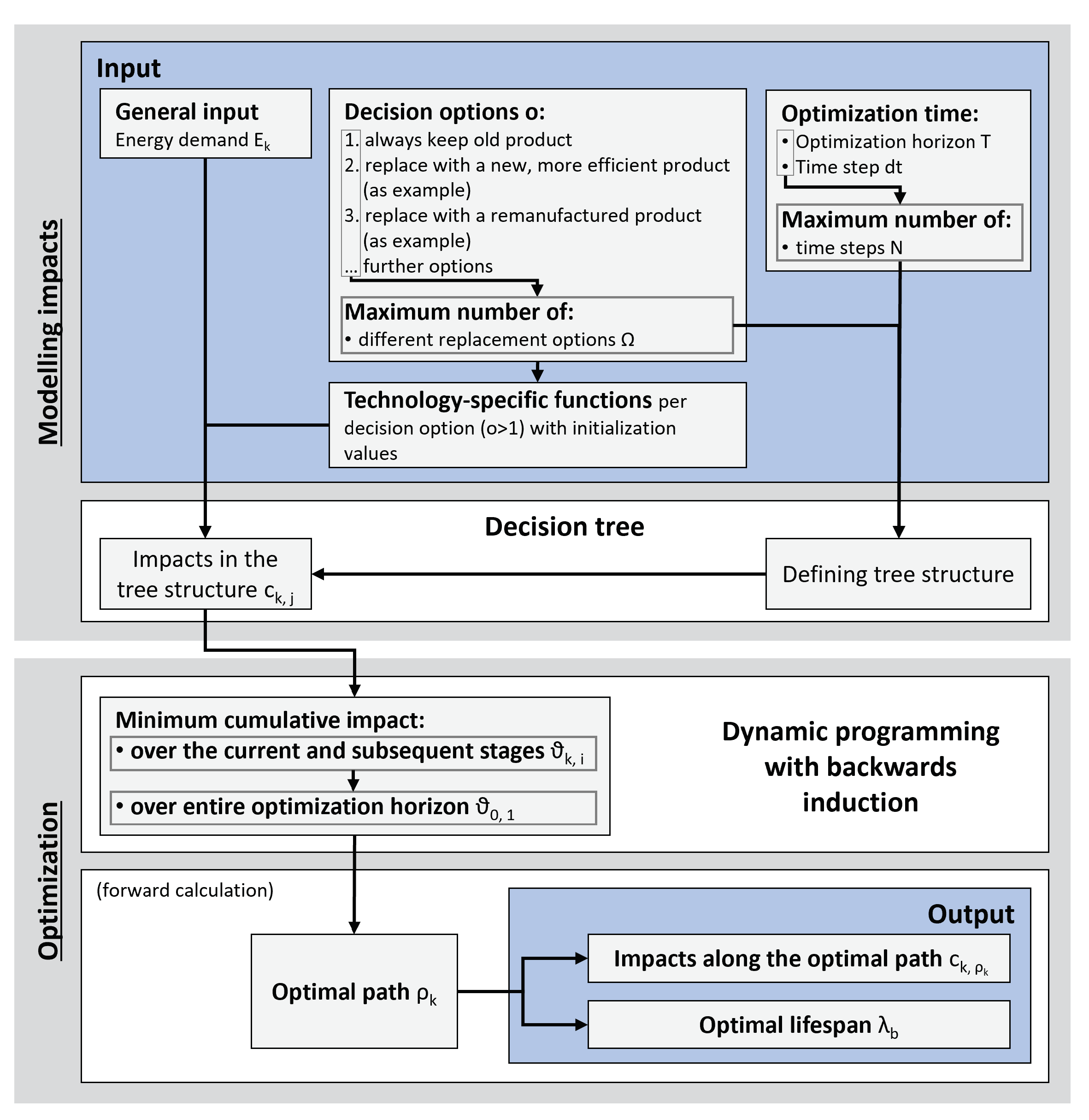
Figure 2.
Decision tree for 3 decision options (, O1: keep old product, O2: replace product with new one, O3: replace product with re-manufactured (r) one) and 3 stages (), with time step, , and impact per time step, (see Section 2.1). The gray dotted extensions at stage N + 1 and the minimum impact for each stage and state, , serve to illustrate the optimization approach (see Section 2.2). Furthermore, the maximum lifespan is chosen to be , resulting in (dashed lines). An exemplary optimal path resulting in minimum cumulative impact at the optimization horizon is highlighted with thick lines: . This results in an optimal lifespan of 2 dt for the first product and of 1 dt for the second product.

Figure 3.
Model structure and baseline scenarios with exemplary illustration for (including a dynamic model of heat demand, technological efficiency progression defining the initial product efficiency and annually differentiated, varying electricity energy mixes) and efficiency degradation, .
Figure 3.
Model structure and baseline scenarios with exemplary illustration for (including a dynamic model of heat demand, technological efficiency progression defining the initial product efficiency and annually differentiated, varying electricity energy mixes) and efficiency degradation, .
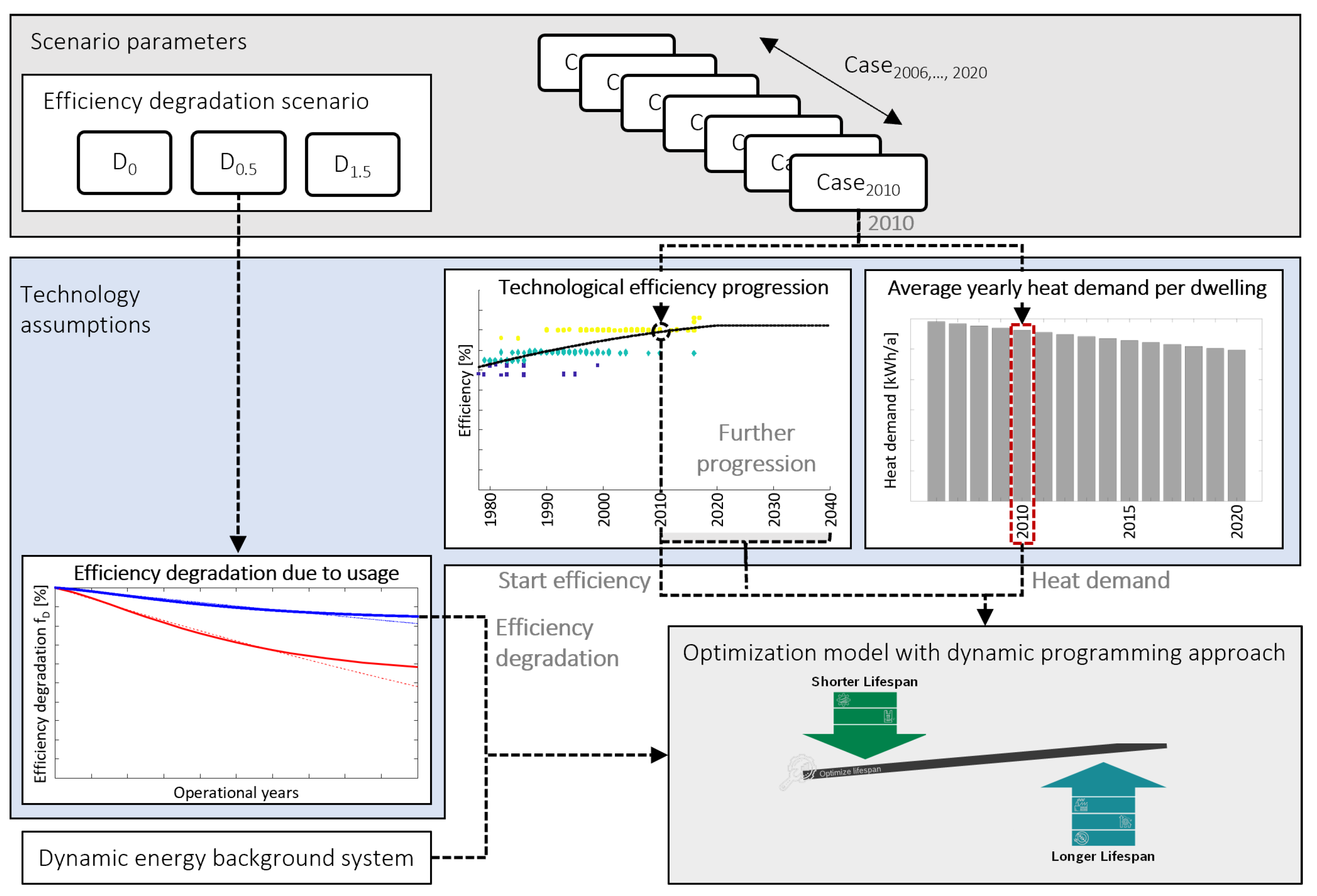
Figure 4.
Overview of the four different infrastructure scenarios () evaluated in the scenario analysis; each differed in the assumed efficiency degradation resulting from different maintenance schedules (, , ) and the first installation year of the product (). The latter defines the start efficiency of the product with potential further technological efficiency progression and annual heat demand. Per-case assessed, all scenario components remain constant.
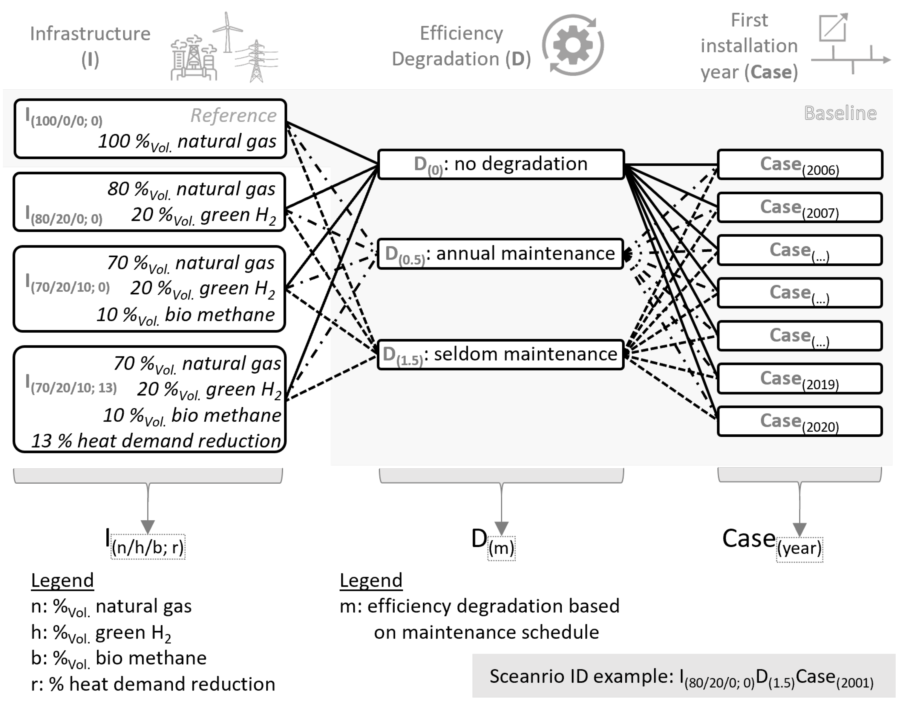
Figure 5.
Climate change impact optimization results for the selected first installation years 2006 () and 2020 () with efficiency degradation assumptions depending on the maintenance schedule scenario (: no efficiency degradation; : annual professional; and : no or seldom maintenance) and two replacement options (; O1: further use of the product; O2: newly evolved gas boiler; O3: re-manufactured gas boiler). The graph shows the impact in each year for the option where the initial boiler is used for 15 years (red dashed line). This is the baseline for comparing the impacts of the replacement scenarios. The (black) solid line shows the optimized impacts that occur each year. Impacts due to the production as well as recycling of a replacement product are also included and result in peaks every year with an exchange. The exchange is also indicated by arrows pointing to filled circles for replacement with a new product (O2) and unfilled squares for replacement with a re-manufactured product (O3). The (gray) area between both graphs is the potentially avoided impact through optimized replacement, and the integral of it is the cumulative avoided impact.
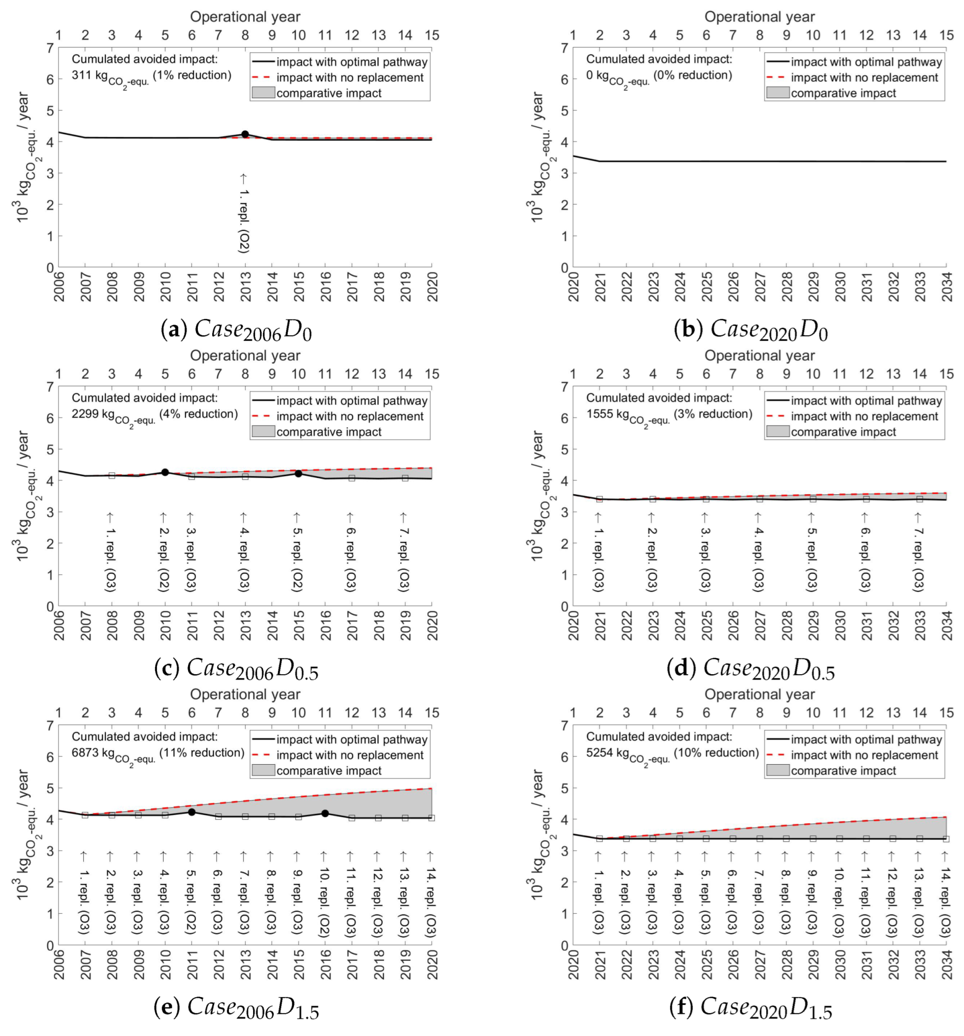
Figure 6.
Distribution of optimal environmental lifespan (OEL) results for climate change impacts (a–c) and (d–f) for all 15 considered cases ( to ) with the respective maintenance schedule (: no efficiency degradation; : annual professional and : so or seldom maintenance) and two replacement options (; O1: further use the product; O2: new, evolved gas boiler; O3: re-manufactured gas boiler). The boxes show the median with a circle as well as the lower and upper quartile, and the whiskers indicate the highest/lowest datum within 1.5 times the interquartile range (Tukey boxplot). Outliers are shown with red crosses.)
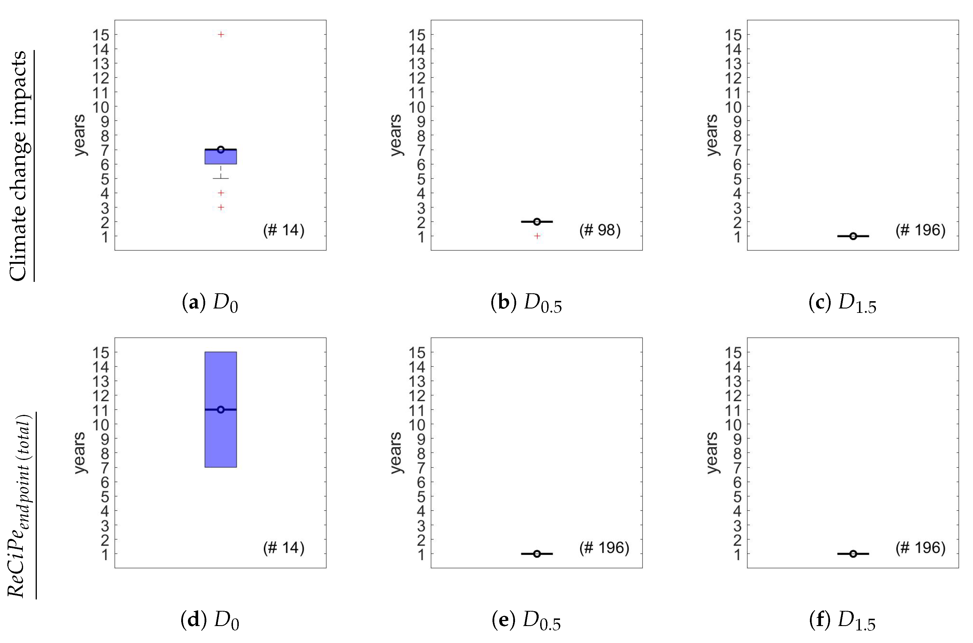
Figure 7.
Total climate change impact reduction potential () over 15 years usage due to improved infrastructure () (e.g., reduced heat demand, decarbonized energy supply) and due to optimized replacement () with two replacement options (; O1: further use of the product; O2: newly evolved gas boiler; O3: re-manufactured gas boiler). Each Tukey boxplot represents the reduction potential per assessed scenario (, see Figure 4 for a scenario overview) of all 15 considered cases (: to ) with the respective maintenance schedule (: no efficiency degradation; : annual professional; and : no or seldom maintenance). is derived according to Thamling et al. [80] and plotted on the third axis. The boxes show the median with a circle as well as the lower and upper quartiles, and the whiskers indicate the highest/lowest datum within 1.5 times the interquartile range (Tukey boxplot). Outliers are not displayed. Boxplots of are truncated at the x-axis for illustration purposes but are actually symmetrical to it. Reading assistance: For example, in scenario with green in the gas mix () and “annual and professional maintenance” (), decarbonization of the infrastructure () contributes to 6% reduction. Under these assumptions, an optimized replacement leads to a median reduction potential of 3% () with a recommended replacement every 2 years on average (median). The median total reduction potential in this scenario is around 9% (: 3rd axis) compared to usage where the product is used for 15 years and no infrastructure improvements are made, but the product is annually and professionally maintained. (The reader is referred to the web version of this article for a figure with higher resolution).
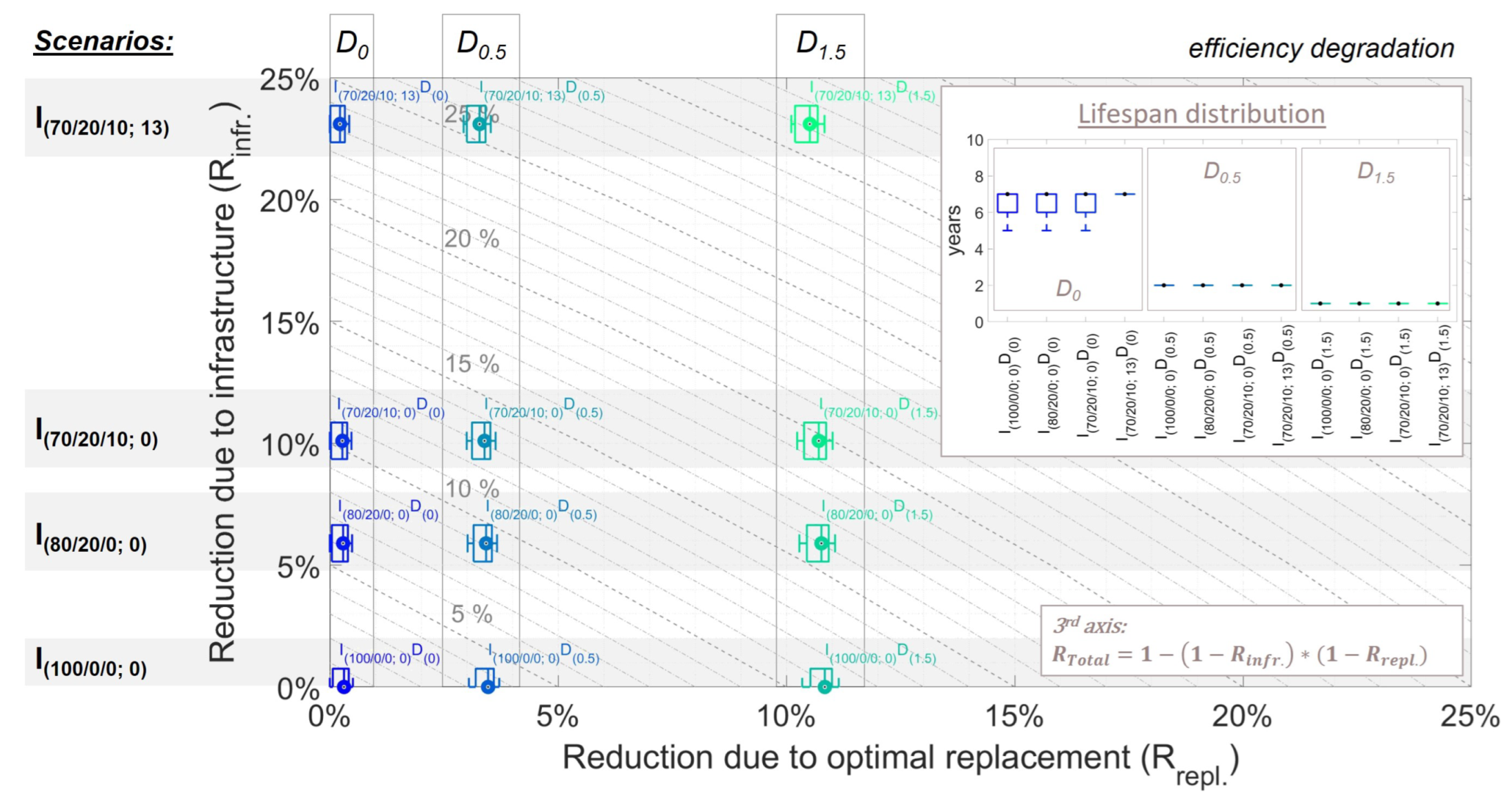

Table 1.
Approaches used in the literature to environmentally optimize replacement options and time (* their life cycle optimization model has been used by many other authors, such as Kim et al. [32], de Kleine et al. [33], Bakker et al. [34]; ** due to simultaneous consideration of efficiency degradation and improvement; one replacement option: keep old or replace with an alternative product).
| Optimization Objective | Mathematical Approach | Reference Authors | Replacements Actions | Replacement Options at the Same Time | Non-Linear Optimization Problem ** | Application in Case Studies |
|---|---|---|---|---|---|---|
| Minimizing impact rate at break-even | Iterative approach with scenario assessment | van Nes and Cramer [14] | one | one | no | - |
| Analytical approach by solving integral | Dewulf and Duflou [18] | one | one | no | Cars, refrigerators | |
| Minimizing cumulative impact over a time horizon | Numerical approach in which derivatives of mathematical series are solved iteratively | Skelton and Allwood [30] | Several with (ir)regular frequency | one | no | Cars, plane, washing machine, office block |
| Dynamic programming | Kim et al. [31] *, Liu et al. [35], Chung et al. [37] | Several with irregular frequency | one | yes | Cars, refrigerators, freezers, washing machines, air conditioners, residential lightning | |
| Scenario assessment (no optimization algorithm) | Ardente and Mathieux [22], Boldoczki et al. [24], Pérez-Belis et al. [36] | one | one | no | Vacuum cleaners, washing machines, refrigerators, freezers, printers, laptops, monitors, PCs |
Disclaimer/Publisher’s Note: The statements, opinions and data contained in all publications are solely those of the individual author(s) and contributor(s) and not of MDPI and/or the editor(s). MDPI and/or the editor(s) disclaim responsibility for any injury to people or property resulting from any ideas, methods, instructions or products referred to in the content. |
© 2023 by the authors. Licensee MDPI, Basel, Switzerland. This article is an open access article distributed under the terms and conditions of the Creative Commons Attribution (CC BY) license (https://creativecommons.org/licenses/by/4.0/).
Share and Cite
MDPI and ACS Style
Hummen, T.; Hellweg, S.; Roshandel, R. Optimizing Lifespan of Circular Products: A Generic Dynamic Programming Approach for Energy-Using Products. Energies 2023, 16, 6711. https://doi.org/10.3390/en16186711
AMA Style
Hummen T, Hellweg S, Roshandel R. Optimizing Lifespan of Circular Products: A Generic Dynamic Programming Approach for Energy-Using Products. Energies. 2023; 16(18):6711. https://doi.org/10.3390/en16186711
Chicago/Turabian StyleHummen, Torsten, Stefanie Hellweg, and Ramin Roshandel. 2023. "Optimizing Lifespan of Circular Products: A Generic Dynamic Programming Approach for Energy-Using Products" Energies 16, no. 18: 6711. https://doi.org/10.3390/en16186711
Note that from the first issue of 2016, this journal uses article numbers instead of page numbers. See further details here.