A Two-Terminal Directional Protection Method for HVDC Transmission Lines of Current Fault Component Based on Improved VMD-Hilbert Transform

Abstract

The traveling wave protection of high voltage direct current (HVDC) transmission lines is susceptible to the influence of transition resistance. As a backup protection, current differential protection has absolute selectivity, but usually requires an increase in delay to avoid misoperation caused by distributed capacitance on the line, resulting in a longer action time. Based on this, a two-terminal directional protection method for HVDC transmission lines is proposed based on Sparrow Search Algorithm (SSA)-Variational Mode Decomposition (VMD) and Hilbert phase difference. On the basis of analyzing the directional characteristics of the current fault component at both ends of the rectifier and inverter sides under different faults, SSA is first used to optimize the parameters of VMD. The residual components representing the direction of the current fault component at both ends are extracted through VMD, and then the Hilbert phase difference of the residual components at both ends is calculated to identify faults inside and outside the line area. In addition, fault pole selection can be achieved based on the ratio of the sum of multi-band Hilbert energy of single-terminal voltage fault components at the positive and negative poles. Simulation experiments have shown that the proposed protection scheme can quickly and effectively identify fault and has good tolerance to transition resistance and noise interference.

1. Introduction

HVDC transmission has the advantages of long transmission distance, large transmission capacity, low line loss, and easy control, which is of great significance for large-scale consumption of renewable energy and the realization of rational allocation of resources in a wide area [1,2]. The DC transmission line is long, the protection device is complex, the fault occurrence rate is high, and the reliable and rapid identification of faults plays a vital role in the safe and stable operation of the whole system. Therefore, research on DC line protection is particularly important [3,4].

Current differential protection, as a backup protection for DC line traveling wave protection and differential undervoltage protection [5,6,7], is mainly used to detect high-resistance grounding faults. Affected by the distributed capacitance of the line, the protection action time can reach up to 1100 ms [8]. In order to improve the sensitivity and rapidity of backup protection, some experts and scholars have conducted extensive research on the time-frequency analysis method for two-terminal electrical quantities protection. Li et al. [9] constructed a two-terminal protection based on the difference in wavelet energy relative entropy of the voltage and current fault components at both ends during internal and external faults, which was difficult to select the basis function of the wavelet transform, and false spectra might appear during decomposition. Shu et al. [10] proposed a protection method based on Principal Component Analysis (PCA) clustering to determine the direction of short circuit faults. Gong et al. [11]. used the terahertz simulation signals processed by PCA downscaling as samples for Elman neural network training to measure the thickness of aero-generator thermal barrier coatings for determining the faults of its thermal cross-section parts. However, the method was sensitive to data distribution, easily affected by outliers, weakly capable of handling complex nonlinear information, and required a sufficient number of samples for clustering accuracy [12], which remained to be explored for wider application in DC line fault identification. Qi et al. [13] analyzed the polarity difference between the fault voltage and current at both ends of the fault by Hilbert-Huang transform, which was more accurate for fault classification. Nevertheless, the method took Empirical Mode Decomposition (EMD) for transient quantities, ignoring the problems of different degrees of modal aliasing and end-point effects that may occur during signal decomposition [14,15], which limited its fault information extraction performance.

In 2014, Dragomiretskiy and Zosso proposed a novel adaptive, fully non-recursive Variational Mode Decomposition (VMD) algorithm based on a recursive model of the EMD algorithm [16]. VMD decomposes multi-component signals into multiple amplitude modulated-frequency modulated (AM-FM) signals by solving a variational constrained model. It is widely used in medical, mechanical, and signal processing [17,18,19], and is often used for fault identification and fault location in engineering fields. Viswanath et al. [20] introduced the VMD algorithm in power signal processing, accurately identifying pulse transients and spike signals in the signal. Wang et al. [21] proposed a novel method combining the VMD algorithm and a Teager energy operator for fault location of hybrid DC lines, which outperformed existing time-frequency analysis methods such as Wavelet Transform (WT) and Ensemble Empirical Mode Decomposition (EEMD). Xu et al. [22] discussed the effectiveness of the VMD algorithm in extracting fault information and decomposed multiple power quality disturbance waveforms to extract their feature information. Luo et al. [23] detected and analyzed the ripple components of complex DC signals by a combination of VMD and Hilbert transform. Compared with the EMD algorithm, the VMD algorithm detected more accurately under noisy conditions. In order to improve the fault location accuracy, Wang et al. [24] introduced the VMD feature quantity into a kind of fault location model based on a deep hybrid Convolutional Neural Network (CNN) and a Long Short-Term Memory (LSTM) network, which effectively improved the learning effect of the model.

The combination of VMD and Hilbert transform is a kind of adaptive time-frequency analysis method based on the improvement of the Hilbert-Huang transform [25], which overcomes the problem of large computational errors for the Hilbert transform caused by the error of EMD modal components. It can perform the Hilbert transform on each single-component modal signal decomposed by VMD and extract the fault eigenvalues, and it has been widely used in signal analysis of the power system. Paternina et al. [26] introduced VMD to identify the electromechanical oscillation mode by using the instantaneous modal eigenvalues of the oscillating power signals obtained by the Hilbert transform. In order to reduce the photovoltaic power fluctuation rate under different weather conditions, Xiao et al. [27] used the VMD-Hilbert transform to adaptively allocate the power from the hybrid energy storage system (HESS) to lead-carbon batteries and supercapacitors. Zhang et al. [28] took VMD to conduct feature analysis on the fault transient signal of the positive sequence current, extracted the fault feature vectors through Hilbert transformation, and used them as the input of CNN to establish a fault diagnosis model. Based on a large number of studies, it is found that the number of modal components K and the quadratic penalty factor α of the VMD algorithm have a great influence on the results. However, since the parameters of the VMD algorithm are mostly selected by relying on experience, too much deviation in the parameter selection can lead to distortion of the decomposition results and extraction of inaccurate fault information.

In this paper, a novel two-terminal directional protection method for HVDC transmission lines of current fault component based on improved VMD-Hilbert transform is proposed according to the directional characteristics of the current fault component at both ends of the line. First, the SSA optimization algorithm is used to optimize the two key parameters of VMD by taking the average envelope entropy of the modal components after the decomposition of the original signal as the objective function. Subsequently, the line protection criterion is constructed from the Hilbert phase angle difference of the current fault component at both ends by the VMD-Hilbert transform. Meanwhile, the ratio of the sum of multi-band Hilbert energy of single-terminal voltage fault components at the positive and negative poles are utilized for the fault pole selection. Finally, a simulation model of the Yunnan-Guangzhou ±800 kV ultra-HVDC transmission line is constructed in PSCAD/EMTDC, and the feasibility of the protection scheme is verified under different fault types. Simulation results show that the proposed scheme can correctly identify the faults inside and outside the HVDC line area without the influence of distributed capacitance and the limitation of fault and has good tolerance to transition resistance and noise interference, which is an excellent novel method for time-frequency analysis.

2. Basic Principles of Improving VMD-Hilbert Transform

2.1. Algorithmic Principles of the VMD-Hilbert Transform

VMD is a signal processing algorithm with high resolution and strong robustness, which essentially involves multiple adaptive Wiener filtering groups. The original signal f is decomposed into K intrinsic mode function (IMF) components with independent center frequency in different frequency bands. The mathematical model for variational mode decomposition is

$$\left\{\begin{array}{l}\mathrm{s}.\mathrm{t}.{\displaystyle \sum _{k=1}^K{\mu }_k}=f\\ \underset{\left\{{\mu }_k\right\},\left\{{\omega }_k\right\}}{\min }\left({{\displaystyle \sum _{k=1}^K‖{\partial }_t\left(\left(\delta \left(t\right)+\frac{\mathrm{j}}{\mathsf{\pi }t}\right)\ast {\mu }_k\left(t\right)\right){\mathrm{e}}^{-\mathrm{j}{\omega }_{k}t}‖}}_2^2\right)\end{array}\right.$$

(1)

where f is the original signal; K is the number of modal components; μ_k is the k-th IMF component decomposed by VMD; ω_k is the center frequency of the k-th IMF component; δ(t) is the unit pulse function; and ${‖\cdot ‖}_2^2$ represents L₂ norm operation.

In order to solve the above variational equation, a quadratic penalty factor α and the Lagrange multiplication operator λ are introduced so as to transform Formula (1) into an unconstrained variational problem, whose calculation formula is

$$\begin{array}{ll}L\left(\left\{{\mu }_k\right\},\left\{{\omega }_k\right\},\left\{\lambda \right\}\right)& =\alpha {\displaystyle \sum _{k=1}^K{‖{\partial }_t\left(\left(\delta (t)+\frac{\mathrm{j}}{\mathsf{\pi }t}\right)\ast {\mu }_k(t)\right){\mathrm{e}}^{-\mathrm{j}{\omega }_{k}t}‖}_2^2+}\\ & {‖f(t)-{\displaystyle \sum _{k=1}^K{\mu }_k(t)}‖}_2^2+〈\lambda (t),f(t)-{\displaystyle \sum _{k=1}^K{\mu }_k(t)}〉\end{array}$$

(2)

where $〈x,y〉$ represents the inner product of x and y.

The alternating direction multiplier iterative algorithm can be used to iteratively update μ_k and ω_k to find the optimal solution of the constrained variational model, where n is the number of iterations and the update expression is as follows

$${\mu }_k^{n+1}(\omega )=\frac{f(\omega )-{\displaystyle \sum _{i<k}{\mu }_i^{n+1}(\omega )}-{\displaystyle \sum _{i>k}{\mu }_i^{n+1}(\omega )+\frac{{\lambda }^n(\omega )}{2}}}{1+2\alpha {(\omega -{\omega }_k^n)}^2}$$

(3)

$${\omega }_k^{n+1}=\frac{{\displaystyle {\int }_0^{\infty }\omega {\left|{\mu }_k^{n+1}\right|}^2\mathrm{d}\omega }}{{\displaystyle {\int }_0^{\infty }{\left|{\mu }_k^{n+1}\right|}^2\mathrm{d}\omega }}$$

(4)

Setting the determination accuracy to terminate the iterative update, the μ_k(ω) Fourier inverse transform after the completion of the VMD algorithm is μ_k(t), which can be used to solve for the K IMF components, and then Hilbert transform them to obtain

$$y(t)=\frac{1}{\mathsf{\pi }}{\displaystyle {\int }_{-\infty }^{\infty }\frac{{\mu }_k(\tau )}{t-\tau }d\tau }$$

(5)

where y(t) is derived from the convolution of μ_k(t) and 1/t. In order to better show the local features of the signal, the analytic function z(t) is constructed as

$$z(t)={\mu }_k(t)+\mathrm{j}y(t)=\beta (t){\mathrm{e}}^{\mathrm{j}\theta (t)}$$

(6)

The instantaneous amplitude β(t), instantaneous phase angle θ(t), and instantaneous angular frequency ω(t) of the analytic function z(t) are, respectively

$$\beta (t)=\sqrt{{\mu }_k{(t)}^2+y{(t)}^2}$$

(7)

$$\theta (t)=\arctan \frac{y(t)}{{\mu }_k(t)}$$

(8)

$$\omega (t)=\frac{d\theta (t)}{dt}$$

(9)

From this, another expression for the original signal f(t) can be derived as

$$f(t)=\mathrm{Re}\left({\displaystyle \sum _{k=1}^{K-1}{\beta }_k(t){\mathrm{e}}^{\mathrm{j}{\displaystyle \int {\omega }_{k}d\omega }}}+r_K(t)\right)$$

(10)

where Re denotes taking the real part; β_k(t) and ω_k(t) are the instantaneous amplitude and instantaneous angular frequency of the k-th IMF component, respectively, and r_K(t) is the residual component.

Omitting the residual components, the Hilbert spectrum H(ω, t) reflecting the time-frequency distribution of the signal amplitude can be obtained as

$$H(\omega ,t)=\mathrm{Re}{\displaystyle \sum _{k=1}^{K-1}{\beta }_k(t){\mathrm{e}}^{\mathrm{j}{\displaystyle \int {\omega }_{k}d\omega }}}$$

(11)

Given that the Hilbert transform can accurately extract the amplitude information of the signal at different frequencies, the Hilbert instantaneous energy E(t) of the signal in any frequency band and its Hilbert energy sum E can be obtained as

$$E(t)={\displaystyle {\int }_{{\omega }_1}^{{\omega }_2}{H}^2(\omega ,t)\mathrm{d}\omega }$$

(12)

$$E={\displaystyle {\int }_{t_1}^{t_2}E(t)dt}$$

(13)

where ω₁ and ω₂ are the angular frequencies; t₁ and t₂ are the starting and ending moments of the fault sampling time, respectively; E(t) is the Hilbert energy as a function of time in a certain frequency band; E is the sum of Hilbert energies during the fault sampling time in a certain frequency band.

2.2. Parameter Optimization of the VMD Algorithm

In practice, the VMD algorithm first selects the appropriate number of modal components K and the quadratic penalty factor α. Determining the values of K and α only empirically results in a certain bias in the decomposition results. If K is set too small, it will cause incomplete decomposition and produce modal aliasing, and if K is too large, it will lead to over-decomposition and produce useless spurious components. The quadratic penalty factor α determines the bandwidth of the IMF for each modal component. If α is set too small, it will cause the IMF component bandwidth to be too large and cause overlapping between components, and if α is too large, it will cause the IMF component bandwidth to be too small resulting in the loss of some signal details. Sparrow Search Algorithm (SSA) is a population intelligence optimization algorithm based on the study of sparrow foraging and anti-predation [29], which has a better performance in convergence speed, accuracy and optimality searching ability and is easy to implement compared to Genetic Algorithm (GA) [30], Particle Swarm Optimization (PSO) [31], Differential Evolutionary (DE) Algorithm [32], etc. In order to be able to accurately find the optimal combination of (K, α), this paper applies SSA to the VMD algorithm for parameter optimization, and its computational principle is shown below.

Discoverers in SSA will constantly search for food to expand their search scope, and their location updates are as follows

$$x_{ih}^{l+1}=\left\{\begin{array}{ll}{x}_{ih}^l·\exp \left(\frac{-i}{\gamma · P}\right),& R_2<S_t\\ x_{ih}^l+Q\mathit{L},& R_2\ge S_t\end{array}\right.$$

(14)

where l is the current iteration number; P is the maximum iteration number; $x_{ih}^l$ is the i-th sparrow of dimension h at the l-th iteration; γ is a random number of (0, 1]; R₂ is the alarm value; S_t is the iteration target value of [0.5, 1]; Q is a random number obeying a normal distribution; and L is a 1 × h matrix with all its elements 1.

The position of the follower in the SSA is updated as follows

$$x_{ih}^{l+1}=\left\{\begin{array}{ll}Q·\exp \left(\frac{x{\omega }_h^l-x_{ih}^l}{i^2}\right),& i>\frac{n}{2}\\ x{b}_h^{l+1}+\left|x_{ih}^l-x{b}_h^{l+1}\right|{\mathit{A}}^{+}·\mathit{L},& i\le \frac{n}{2}\end{array}\right.$$

(15)

where n is the number of sparrows; A⁺ = A^T(AA^T)⁻¹, and A is a 1 × h matrix randomly set to 1 or −1; x${\omega }_h^l$ is the worst position of the sparrow in the h-th dimension at the l-th iteration of the population; and x$b_h^{l+1}$ is the optimal position of the sparrow in the h-th dimension at the (l + 1)-th iteration of the population.

The initial locations of the alarms are randomly generated, typically representing 10–20% of the total sparrow population, and their locations are updated as follows

$$x_{ih}^{l+1}=\left\{\begin{array}{ll}x{b}_h^l+\eta \left(x_{ih}^l-x{b}_h^l\right),& f_i\ne f_g\\ x_{ih}^l+J\left|\frac{x_{ih}^l-x{\omega }_h^l}{\left|f_i-f_w\right|+e}\right|,& f_i=f_g\end{array}\right.$$

(16)

where η is a step control parameter; J is a random number of [−1, 1]; e is a minimal constant; f_i is the fitness value of the i-th sparrow, f_g and f_w are the optimal and worst fitness values of the current sparrow population, respectively.

The average envelope entropy is used as a fitness function to evaluate whether the optimization result is optimal, specifically referring to the average value of the envelope entropy of each modal component obtained by the VMD after decomposing the signal under the parameter combination (K, α), which represents the sparse characteristics of the original signal. The smaller the average envelope entropy represents, the richer the embedded signal information and the better the decomposition effect. The calculation formula is as follows

$$(\widehat{K},\widehat{\alpha })=\underset{(n,P)}{\mathrm{argmin}}\left(\frac{1}{K}{\displaystyle \sum _{k=1}^K{S}_k}\right)$$

(17)

where $\widehat{K}$ and $\widehat{\alpha }$ are the optimal parameter combinations; S_k is the envelope entropy of each modal component after Hilbert demodulation; S_k(i) is calculated as follows

$$S_k(i)=-{\displaystyle \sum _{i=1}^{N}p(i){\log }_2\left[p(i)\right]}$$

(18)

$$p_i=c(i)/{\displaystyle \sum _{i=1}^{N}c(i)}$$

(19)

where i = 1,2, …, N, N is the number of sampling points; p(i) is the normalized form of c(i); c(i) is the envelope signal after the original signal is Hilbert transformed.

3. DC Line Fault Discrimination Based on an Improved VMD-Hilbert Transform

For conventional current differential protection, the protection can only operate when the local pole line fault enters the steady state phase. During the fault transient process, the amount of current mutation at both ends of the line has an obvious difference in direction characteristics. Fault direction information can be extracted using time-frequency analysis to realize fault discrimination before control system action. For the above analysis, a DC line protection method based on an improved VMD-Hilbert transform is proposed.

3.1. Analysis of the Direction Characteristics of the Current Fault Component

In this paper, a positive DC line is used as an example, and its simplified equivalent circuit is replaced by a centralized parametric model that takes into account the effect of capacitive currents. When an in- and out-of-area fault occurs on a DC line, the voltage drop at the fault point is equivalent to superimposing a negative voltage source at the fault point, and the fault-attached network is shown in Figure 1. In Figure 1, Z_l and C_eg are DC line equivalent impedance and ground equivalent capacitance; Z_f, Z_s, and Z_c are the DC filter, the leveling reactor, and converter equivalent impedance; u_f is the equivalent additional voltage source voltage at the fault point; Δi_R and Δi_I are the rectifier side and inverter side of the current fault component during the fault, and uniformly stipulate that the positive direction of the current is from the busbar to the line.

It can be seen from Figure 1 that when there is an internal fault in the line area, under the action of the fault equivalent additional voltage source, the current fault component Δi_R and Δi_I at both ends flows from the bus to the line, and both directions are the same, both are positive, Δi_R > 0, Δi_I > 0; when there is an external fault on the rectifier valve side, also under the action of the fault equivalent additional voltage source, the direction of the rectification side current fault component Δi_R is pointing to the bus, and the direction of the inverter side current fault component Δi_I is pointing to the line, and both directions are opposite, Δi_R > 0, Δi_I < 0; when there is an external fault on the inverter valve side also under the action of the fault equivalent additional voltage source, the direction of the current fault component Δi_R on the rectifier side is pointing to the line, and the direction of the current fault component Δi_I on the inverter side is pointing to the bus, and both directions are opposite, Δi_R < 0, Δi_I > 0. The analysis of bipolar inter-pole short circuits and AC bus external faults is similar and will not be repeated. Therefore, the use of the direction characteristics of the current fault component at both ends of the line can be used for the identification of faults inside and outside the DC line area.

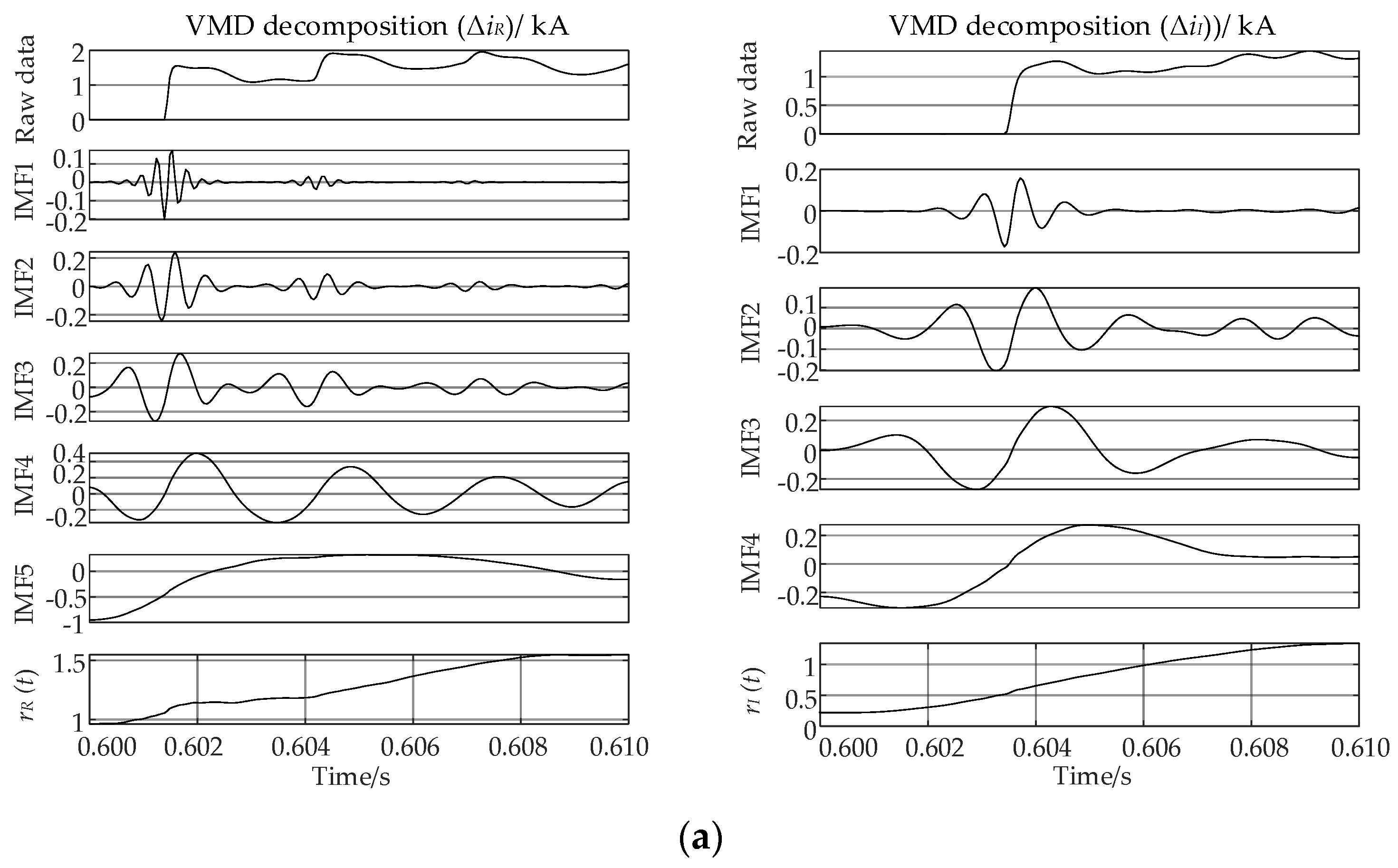
3.2. SSA-VMD Extraction of Residual Components

When a fault occurs on a DC line, the waveform of the current fault component often does not vary smoothly and monotonically. Due to the significant difference in the oscillation frequency of the fault current at the beginning and end of the line, as well as the distributed capacitance and channel noise of the line, the polarity difference of the current sudden variable fluctuates, making it difficult to effectively characterize the trend of signal changes. However, the VMD algorithm is able to adaptively smooth non-stationary signals based on the local variation characteristics of the signal, effectively filtering out the volatility. According to the theory in Section 2.1, the original signal f(t) is decomposed into the superposition of various IMF components and residual components, with the expression as follows

$$f(t)={\displaystyle \sum _{k=1}^{K-1}{\mu }_k(t)+r_K(t)}$$

(20)

where μ_k(t) is the IMF component of each order arranged from high frequency to low frequency, reflecting the volatility of the current fault component; the residual component r_K(t) characterizes the average trend of the signal, reflecting the direction of change of the current fault component.

Optimization of the parameters of the VMD algorithm using SSA according to different fault types, respectively, the optimal parameter combinations ($\widehat{K}$, $\widehat{\alpha }$) can be obtained for different fault types. The number of the sparrow population is set to 80, the maximum number of iterations is 20, and the upper and lower limits of K and α are [3, 20] and [20, 2500], respectively. Figure A1 of Appendix A shows the adaptive curve for optimization of the parameters of the current fault component at both ends of the line during an internal fault in the DC line, which basically reaches stability after three iterations, and the optimal values of the adaptivity function are 3.7389 and 4.165, respectively. Some of the optimal parameter combinations for different fault types after optimization are shown in

Table 1. Parameter optimization under different fault types.

Type of Fault	Fault Distance/km	Transition Resistance/Ω	$\mathbf{Rectifier}\mathbf{Side}(\widehat{\mathit{K}}$$,\widehat{\mathit{\alpha }}$)	$\mathbf{Inverter}\mathbf{Side}(\widehat{\mathit{K}}$$,\widehat{\mathit{\alpha }}$)
Internal fault in the line area	400	10	(7, 173)	(6, 78)
		100	(6, 345)	(5, 89)
		300	(6, 107)	(5, 35)
	700	10	(4, 341)	(5, 183)
		100	(4, 210)	(4, 155)
		300	(4, 97)	(4, 104)
	1300	10	(7, 241)	(8, 541)
		100	(6, 99)	(8, 346)
		300	(6, 153)	(7, 301)
External fault on rectifier valve side	–	10	(10, 2251)	(9, 211)
	–	100	(11, 1544)	(9, 194)
External fault on inverter valve side	–	10	(8, 351)	(10, 658)
	–	100	(8, 222)	(9, 514)
Three-phase failure of the AC bus on the rectifier side	–	–	(9, 189)	(7, 58)
Three-phase fault of the AC bus on the inverter side	–	–	(7, 115)	(7, 258)

.

The VMD parameters are optimized to decompose the current mutation at both ends of the line during faults inside and outside the line area, and the fault moment is set to be t = 0.6 s, the time window length is 10 ms, and the sampling frequency is 20 kHz. The VMD decomposition of the current fault component at both ends of the line for an internal fault 400 km from the rectifier side (transition resistance of 100 Ω) and an external fault on the rectifier valve side (transition resistance of 10 Ω) are given in Figure 2, respectively. The residual components r_R(t) and r_I(t) at the ends of the rectifier and inverter sides can reflect the direction of change of the current fault component. As can be seen from Figure 2, the waveforms of each modal component decomposed by the VMD are clear, both high-frequency and low-frequency components are accurately decomposed, and the extracted residual components are monotonic.

3.3. Directional Determination Based on Phase Angle Difference of Hilbert Transform

According to the analysis in Section 2.2, it can be shown that the residual components r_R(t) and r_I(t), which are obtained after the two-terminal current fault component Δi_R and Δi_I are decomposed by the VMD, can characterize the mutation direction of the fault signal. Therefore, taking the conclusion of Section 2.1 as a reference, it is proposed to utilize the Hilbert phase angle difference of the residual components of the current fault component at both ends to reflect the difference in the direction of the current fault component after a fault, and to take the Hilbert phase angle difference as a characteristic quantity for discriminating faults inside and outside the line area. Figure 3 shows the Hilbert transform results of the residual components r_R(t) and r_I(t) at both ends for faults inside and outside the DC line area, and the fault types are consistent with Section 2.2.

The residual components obtained after the Hilbert transform have better time-frequency resolution characteristics, which can provide complete transient information with good identification accuracy. It can be seen from Figure 3 that the monotonicity of the residual component affects the size of the Hilbert phase angle. For internal fault, the difference in Hilbert phase angles of the residual components calculated at both ends is small because the direction of the current fault component at both ends is positive and the transmission time of the data at both ends is taken into account. When an external fault occurs, the Hilbert phase angles of the residual components at the both ends obtained from subsequent calculations differ significantly due to the opposite direction of the current fault component at the both ends.

3.4. Directional Protection Criterion of the Current Fault Component Based on an Improved VMD-Hilbert Transform

There are four HVDC line protection devices, which are, respectively, installed at the beginning and end of the positive line and the beginning and end of the negative line. The line acquisition protection device obtains the current fault component at both ends of the positive and negative lines and the voltage fault component on the rectifier side of the positive and negative lines. The relevant criteria are defined as follows: the start criterion is the triggering condition of the protection process, the action criterion is the discriminating condition for recognizing internal and external faults, and the fault pole selection criterion is the discriminating condition for recognizing the faulty pole of the line.

• Start criterion:

Construct a pole current protection activation criterion based on the value of the current fault component. Due to load and grid frequency fluctuations, the degree of fluctuation of the pole current is less than 8% of the rated current IN during normal operation of the system. Let I_set = 0.08I_N, when the degree of fluctuation of the pole current Δi_φ is greater than the set current I_set, the protection is activated, as follows

$$\Delta i_{\phi }>I_{\mathrm{set}}$$

(21)

2.

Action criterion:

From the above analysis, it is clear that the directional characteristics of the current components at both ends of the line are different when internal and external faults occur on the DC line. If the waveform of the fault transient signal is used directly to determine the direction, the protection may misjudge when lightning interference occurs, and it is difficult for the protection to cover the entire length of the line. In this regard, based on the theory in Section 1, it is proposed to utilize the improved VMD-Hilbert transform phase angle difference to discriminate the directional characteristics of the current fault component after a fault, and then to identify whether or not an internal fault occurs in the line. The method first calculates the Hilbert phase angle of the current fault component for each sampling point in the data window and then finds the phase angle difference between both. In order to reduce the influence of interference and improve the stability of data analysis, the Hilbert phase angle difference at both ends was mean smoothed. After the discretization process, the action criterion of the protection is defined as

$$\Delta {\theta }_i=\frac{1}{N}{\displaystyle \sum _{n=1}^N\left|{\theta }_{Ri}(n)-{\theta }_{Ii}(n)\right|}$$

(22)

where: i = 1,2 represents the positive and negative poles; θ_Ri(n), θ_Ii(n) represent the Hilbert phase angles of the current fault component of the rectifier side and the inverter side at the n-th sampling point on the i-pole, respectively and Δθ_i is the average of the absolute value of the difference of the Hilbert phase angles of both ends under the N sampling points.

According to Formula (22) and combined with the characterization of the direction of the current fault component in Section 2.1, it can be seen that the Hilbert phase angle difference between the residual component r_R(t) and r_I(t) at both ends during an internal fault is theoretically equal to 180°; in the case of an external fault, the difference in phase angle between the both their phase angle difference is theoretically equal to 0°. In practice, considering the asynchronous transmission time of data at both ends, the protection needs to be set with sufficient margin to ensure reliable operation. Considering the sensitivity and reliability, the following criterion can be constructed

$$\left\{\begin{array}{ll}\mathrm{Internal}\mathrm{fault}:& 0^{°}\le \Delta {\theta }_i\le {50}^{°}\\ \mathrm{External}\mathrm{fault}:& {150}^{°}\le \Delta {\theta }_i\le {200}^{°}\end{array}\right.$$

(23)

In Formula (23), the protection only through the two-terminal fault quantities of the Hilbert phase angle difference of the direction of the discriminant value to identify the fault, the signal synchronization requirements are low, with a certain anti-interference ability, compared with the traditional time-frequency analysis method has a better adaptive resolution ability.

3.

Fault pole selection criterion

For the bipolar DC system, when a single pole fault occurs on the overhead line, the voltage and current fault components are also detected on the sound pole due to the electromagnetic coupling between the two poles of the line, and the method of selecting the fault poles cannot be realized by using only the Hilbert phase angle difference. This paper introduces the method of identifying faulty poles using only the voltage fault component signal. Theory and simulation show that the energy of the post-fault voltage fault component is mainly concentrated in the low-frequency band, and the coupling coefficient of the two poles of the line is the largest when the frequency is 500~2000 Hz [33]. Due to the frequency-varying nature of the series impedance and shunt conductance of the transmission line, the high-frequency energy of the voltage fault component is greater than that of the sound pole. From this, a pole selection criterion can be constructed using the ratio of the high- and low-frequency Hilbert energy sums of the positive and negative single-ended voltage fault components. Figure A2 and Figure A3 of Appendix B show the multi-band Hilbert instantaneous energy diagrams of voltage fault component on the rectifier side of the positive and negative poles during internal and external faults on the DC line, respectively, and the fault types are the same as in Section 2.2. The pole selection factor P is defined as

$$P=\frac{E_{Rl1}+E_{Rh1}}{E_{Rl2}+E_{Rh2}}=\frac{E_{R1}}{E_{R2}}$$

(24)

where E_Rl1, E_Rh1 are the low-frequency Hilbert energy (1~500 Hz) and high-frequency Hilbert energy (6~10 kHz) of the voltage fault component on the positive rectifier side of the line; E_Rh2, E_Rl2 are the high and low-frequency Hilbert energy of the voltage fault component on the negative rectifier side of the line; and E_R1, E_R2 are the sum of the high and low-frequency Hilbert energy of the voltage fault component on the positive and negative rectifier sides of the line, respectively.

From this, a multi-band Hilbert energy sum ratio based on the positive and negative single-ended voltage fault component can be constructed as a fault pole selection criterion, expressed as follows

$$\left\{\begin{array}{ll}\mathrm{positive}\hspace{0.17em}\mathrm{fault}:& P\ge P_{\mathrm{set}1}\\ \mathrm{negative}\mathrm{fault}\hspace{0.17em}:& P\le P_{\mathrm{set}2}\\ \mathrm{bipolar}\hspace{0.17em}\hspace{0.17em}\mathrm{fault}:& P_{\mathrm{set}2}\le P\le P_{\mathrm{set}1}\end{array}\right.$$

(25)

where P_set1 and P_set2 are the upper and lower thresholds of the criterion, considering a certain margin, P_set1 takes the value of 1.2, and P_set2 takes the value of 0.95.

Summarizing the above, the two-terminal protection method for HVDC lines based on the improved VMD-Hilbert current fault component direction proposed in this paper is shown in Figure 4.

4. Simulation Analysis of the Experiments

4.1. Simulation Model of the HVDC Transmission System

According to the actual parameters of the Yunnan-Guangzhou ± 800 kV Ultra-HVDC transmission system, a simulation model of the bipolar HVDC system shown in Figure 5 is constructed in PSCAD/EMTDC, with a voltage level of ±800 kV and a rated current of 3.125 kA. Both the rectifier and inverter stations have a rated capacity of 2000 MW and use 12-pulse wave converter valves; the line is modeled in the frequency modal domain, with a total length of 1418 km and 6 splits; the rectifier station adopts constant current and constant trigger angle control, while the inverter station adopts constant current and constant arc quenching angle control, and at the same time, low voltage current limiting modules are installed at both ends.

In Figure 5, f1 and f2 are positive and negative DC line internal faults; f3 is a bipolar fault; f4 and f6 are positive and negative rectifier valve-side faults; f5 and f7 are positive and negative inverter valve-side faults; and f8 and f9 are three-phase short-circuit faults on the AC bus. In this paper, the simulation analysis sets the fault moment as t = 0.6 s, the time window length as 10 ms, the sampling frequency as 20 kHz, and the simulation analysis is carried out for different fault types using SSA-VMD and Hilbert transform.

4.2. Simulation of Internal Faults in the Line Area

The current fault component, residual components, and their Hilbert phase angle results of both ends of the rectifier and inverter sides at the positive line are shown in Figure 6 and Figure 7, respectively, when the DC line has a f₁ positive ground fault (transition resistance of 100 Ω) and a f₃ bipolar fault (transition resistance of 10 Ω) at 400 km. The residual components of the current fault component at both ends at the positive line are characterized in the positive direction during the 10 ms time window after the fault, consistent with the analysis in Section 2.1.

The Hilbert phase angle difference can be calculated based on the Hilbert phase angle of the current fault component at each sampling point under the fault and combining it with Formula (22). In Figure 6, the Hilbert phase angle difference Δθ₁ of the residual components at both ends is 4.7553°, and the multi-band Hilbert energy sums of E_R1 and E_R2 of the voltage fault component at the positive and negative rectifier sides are 3.1623 × 107 and 5.9243 × 105, respectively, and then the identification factor P can be obtained to be 53.3783, which fulfills the positive pole fault action criterion. In Figure 7, the Hilbert phase angle difference Δθ₁ of the residual components at both ends is 3.6599°, E_R1 and E_R2 are 4.1404 × 107 and 4.1165 × 107, respectively, which calculates P to be 1.0058, and the protection is determined to be a bipolar fault.

When an internal fault occurs in the negative line, the effects of different fault distances and different transition resistances on fault identification are examined, as shown by the simulation results in

Table 2. Simulation results of faults on the negative line.

Fault Position	Transition Resistance/Ω	Hilbert Phase Angle Difference Δθ2/°	Electrode Selection Factor P	Identification Result
20 km	10	38.0279	0.0416	Negative internal fault
	100	36.4295	0.0223	Negative internal fault
	300	34.1124	0.0719	Negative internal fault
100 km	10	26.7622	0.0693	Negative internal fault
	100	25.2729	0.0545	Negative internal fault
	300	23.6231	0.0414	Negative internal fault
300 km	10	14.1787	0.0294	Negative internal fault
	100	22.5746	0.0202	Negative internal fault
	300	22.4879	0.0583	Negative internal fault
700 km	10	1.0162	0.0192	Negative internal fault
	100	0.1877	0.0361	Negative internal fault
	300	0.3662	0.0682	Negative internal fault
1300 km	10	13.3134	0.0634	Negative internal fault
	100	12.8028	0.1125	Negative internal fault
	300	18.3977	0.1265	Negative internal fault

:

(1)

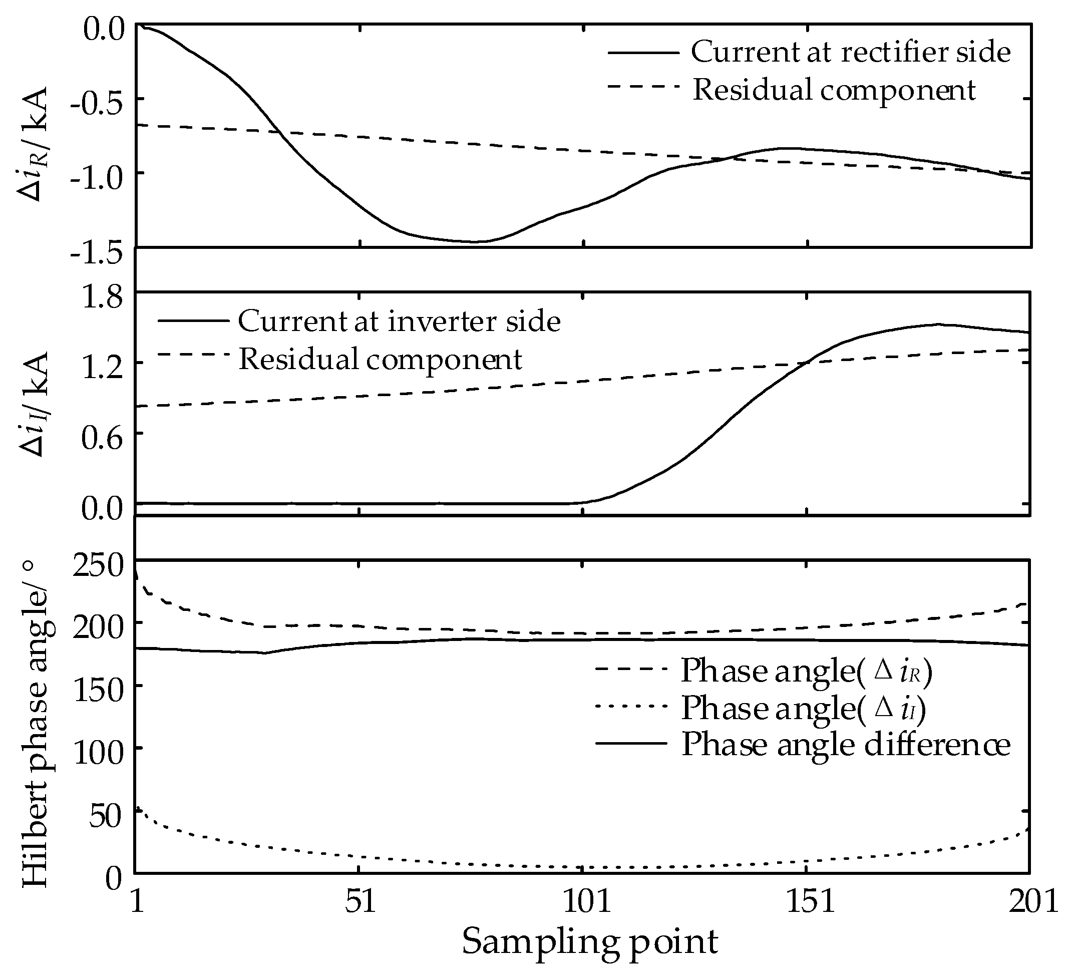
Under different fault distances and transition resistances, the protection can correctly determine the fault section and fault pole.

(2)

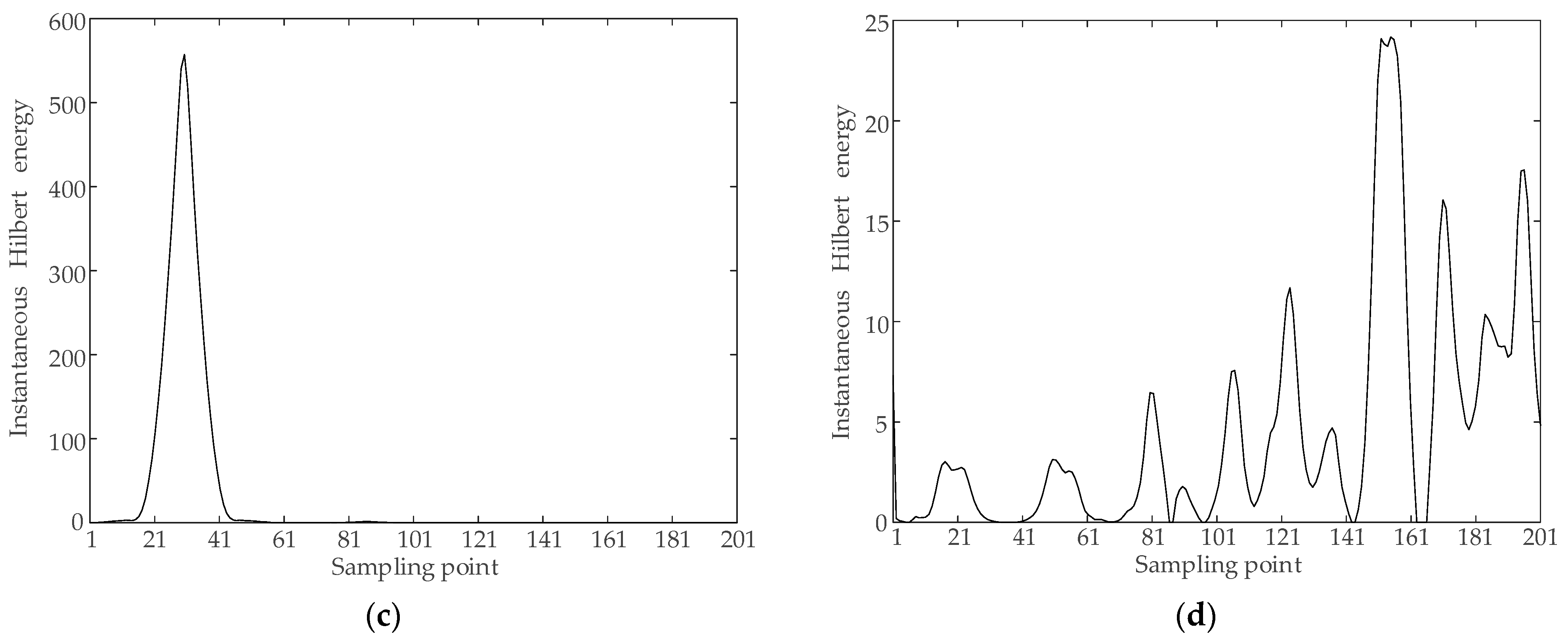
The Hilbert phase angle difference Δθ₂ gradually increases from the midpoint of the line to both ends and when the distance to both ends is 100 km or less, the frequency oscillation of the current fault component causes Δθ₂ to increase faster, which is significantly more on the rectifier side than on the inverter side.

(3)

SSA-VMD of the current fault component eliminates the effects of line distribution capacitance and communication noise, and reliably identifies faults at both ends of the line.

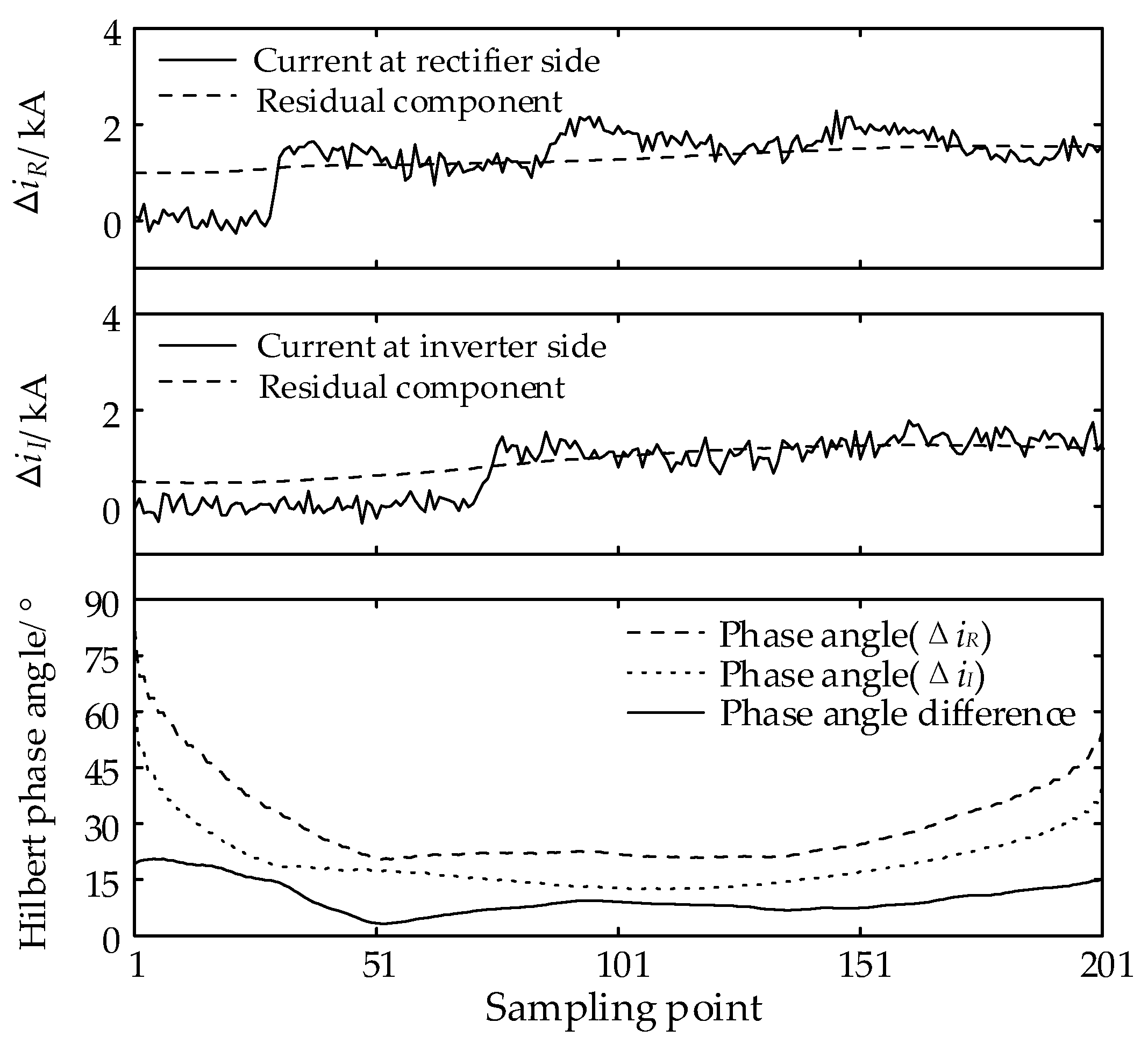
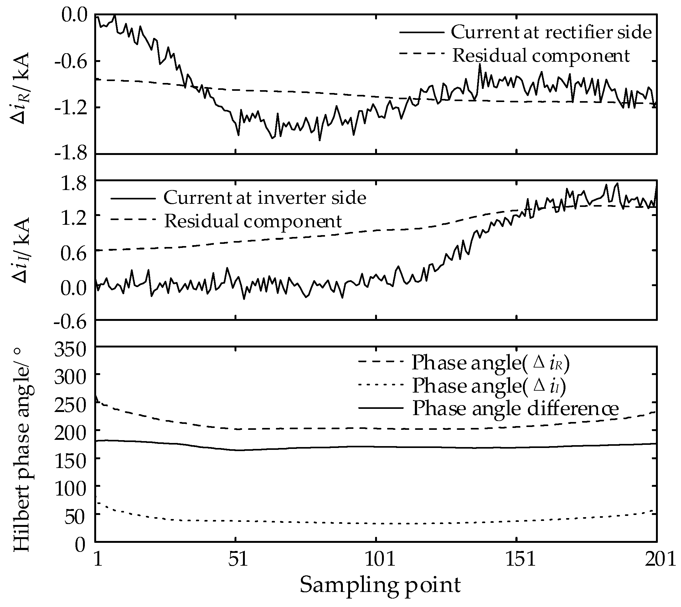
4.3. Simulation of External Faults in the Line Area

Figure 8 and Figure 9 show the simulation results of the current fault component, residual components, and their Hilbert phase angles at both ends of the DC line for the positive rectifier valve side fault f₄ and the inverter valve side fault f₅, respectively. The Hilbert phase angle difference Δθ₁ of the residual components at both ends during the external fault is 185.2359° and 190.1289°, respectively, showing opposite polarity, which satisfies the condition of external fault discrimination.

In order to test the effect of different transition resistances on fault identification during an external fault, the positive rectifier valve side and the inverter valve side are set up to experience external faults f₄ and f₅, as well as the three-phase faults f₈ and f₉ at the AC bus, which are set up to have transition resistances of 10 Ω, 100 Ω, and 300 Ω at the point of the faults, respectively.

Table 3. Simulation results of external faults.

Fault Position	Transition Resistance/Ω	Hilbert Phase Angle Difference Δθ1/°	Hilbert Phase Angle Difference Δθ2/°	Identification Result
f4	10	185.2359	173.6549	External fault
	100	187.3681	177.6515	External fault
	300	182.8825	173.3255	External fault
f5	10	182.1298	170.6549	External fault
	100	181.8433	176.2542	External fault
	300	180.5513	178.9875	External fault
f8	–	183.4566	176.4587	External fault
f9	–	181.1287	173.5422	External fault

shows the Hilbert phase angle differences detected at both ends of the positive and negative lines and the results of the determination.

Due to the high-frequency resistive-band transmission characteristics at the line boundary, the waveforms of the current fault component measured at both ends are smooth, and the two sets of residual components decomposed by the SSA-VMD during external faults are highly directional and show opposite polarities. At the same time, the corresponding Hilbert phase angle is detected on both sides of the sounding pole by the electromagnetic coupling between the DC lines. From the simulation results in Table 3, it can be seen that Δθ₁ and Δθ₂ are both in the 150°~200° interval, and none of the protections will operate incorrectly, which does not affect the fault recognition of this protection.

4.4. Examination of Anti-Noise Interference Performance

In the DC line, two-terminal quantities may introduce noise during transmission over long communication channels. In order to check the noise immunity of the proposed protection scheme, a white noise signal with a signal-to-noise ratio of 10 dB is superimposed on the original current mutation signal. The fault types are set as f₁ positive ground fault (transition resistance of 100 Ω) and f₄ rectifier valve side fault (transition resistance of 10 Ω) in the DC line at 400 km, respectively. From Figure 10 and Figure 11, it can be seen that the white noise signal will cause fluctuations in the amplitude of the fault current, which only exists in the high-level IMF component after VMD, and the trend of the residual component is less affected, and if the parameters of the VMD algorithm are properly selected, the residual component still has the pointing characteristics that characterize the direction of the current fault component. Under the fault condition of superimposed noise interference, the Hilbert phase angle difference Δθ₁ of the residual components at both ends is sought to be 9.9437° and 170.9437°, respectively, and the protection can still reliably discriminate internal and external faults. Therefore, the double-ended protection method proposed in this paper can effectively filter out the fluctuations through SSA-VMD and has certain anti-noise interference capabilities.

4.5. Analysis of Protection Action Time

The two-terminal protection action time is mainly composed of three parts: traveling wave conveyance time difference, channel communication delay, and algorithm calculation time. For a 1418 km long transmission line, the wave speed of the fault traveling wave is approximated to be 98% of the speed of light, and the maximum time difference of the traveling wave conveyed to the measurement points at both ends is about 4.8 ms. In terms of communication delay, the signal transmission rate of dedicated optical fiber communication is about 4.9 μs/km, so the transmission delay of the 1418-km-long optical fiber longitudinal link channel is about 6.9 ms. The algorithm computation time consists of a 10 ms data time window with 0.5 ms computation time, which is approximately 10.5 ms. Taking the above analysis into account and considering the appropriate margin, the total action time of the protection system is about 23 ms, which is earlier than the action time of the control system (about 30 ms) and much faster than that of the current differential protection considering the influence of the distributed capacitance current (about 1100 ms and can better satisfy the requirement of the backup protection of the DC line.

5. Conclusions

This paper proposes a two-terminal current fault component directional protection based on SSA-VMD and Hilbert transform phase angle difference. The feasibility of this protection scheme is evaluated through theoretical analysis and simulation verification, and the results show that this method has the following characteristics:

(1)

VMD combines the features of SSA solving speed and and selects the average envelope entropy as the fitness function to adaptively determine the best selection parameters of VMD, which effectively solves the problem of difficult selection of VMD parameters. Nevertheless, optimization for large-scale complex problems should also be evaluated and tuned on a case-by-case basis.

(2)

SSA-VMD can eliminate the influence of line distributed capacitance and communication noise on the current fault component at both ends of the line, obtain the residual component characterizing the direction of change at both ends, and then calculate the Hilbert phase angle difference through Hilbert transform to determine the directional relationship of the current fault component at both ends of the line. Meanwhile, the ratio of multi-band Hilbert energy sum of single-ended voltage fault component at both poles can be obtained by improving the VMD-Hilbert transform to effectively identify the fault poles.

(3)

Compared with the existing DC differential protection and pilot protection, the proposed protection is not affected by the distributed capacitance and does not depend on the boundary conditions. As verified by simulation, the method does not require a high sampling device and has fast action speed, can reliably identify the internal and external faults, has good tolerance to transition resistance and anti-noise interference, and better meets the backup protection needs of HVDC transmission lines.

(4)

The two-terminal backup protection method proposed in this paper can also be used as the main protection without considering the communication delay and the calculation amount, and can be combined with each other for further analysis in the future. Since the scheme is based on theoretical analysis and simulation verification, it needs to be further combined with actual engineering to verify the applicability of the scheme. At the same time, based on the research in this article, further research can be conducted on this method in related fields of power systems such as lightning strike identification, fault location, fault intelligent algorithm, transient signal analysis, and power quality analysis.

References

1. Perez-Molina, M.J.; Larruskain, D.M.; Lopez, P.E.; Buigues, G.; Valverde, V. Review of Protection Systems for Multi-terminal High Voltage Direct Current Grids. Renew. Sustain. Energy Rev. 2021, 144, 111037. [Google Scholar]
2. Radwan, M.; Azaz, S.P. Protection of Multi-Terminal HVDC Grids: A Comprehensive Review. Energies 2022, 15, 9552. [Google Scholar]
3. Bahrman, M.P.; Johnson, B.K. The ABCs of HVDC Transmission Technologies. IEEE Power Energy Mag. 2007, 5, 32–44. [Google Scholar] [CrossRef]
4. Muniappan, M. A comprehensive Review of DC Fault Protection Methods in HVDC Transmission Systems. Prot. Control. Mod. Power Syst. 2021, 6, 1. [Google Scholar]
5. Zhang, Y.; Tai, N.L.; Xu, B. Fault Analysis and Traveling-Wave Protection Scheme for Bipolar HVDC Lines. IEEE Trans. Power Deliv. 2012, 27, 1583–1591. [Google Scholar] [CrossRef]
6. Gao, B.F.; Zhang, R.X.; Zhang, X.W. A Novel Procedure for Protection Setting in an HVDC System Based on Fault Quantities. J. Electr. Eng. Technol. 2017, 12, 513–521. [Google Scholar] [CrossRef]
7. Gao, S.P.; Liu, Q.; Song, G.B. Current Differential Protection Principle of HVDC Transmission System. IET Gener. Transm. Distrib. 2017, 11, 1286–1292. [Google Scholar] [CrossRef]
8. Lin, S.; Gao, S.; He, Z.Y.; Deng, Y.J. A Pilot Directional Protection for HVDC Transmission Line Based on Relative Entropy of Wavelet Energy. Entropy 2015, 17, 5257–5273. [Google Scholar] [CrossRef]
9. Li, Z.; Zou, G.B.; Du, T.; Yang, W.J. S-Transform Based Pilot Protection Method for HVDC Transmission Lines. In Proceedings of the 2015 5th International Conference on Electric Utility Deregulation and Restructuring and Power Technologies, Changsha, China, 26–29 November 2015; pp. 1667–1672. [Google Scholar]
10. Shu, H.C.; Tian, X.C. Entire-line Instant Protection Based on PCA Clustering for 800kV HVDC Transmission Line. Electr. Power Autom. Equip. 2016, 36, 51–59. [Google Scholar]
11. Gong, Y.L.; Cao, B.H.; Zhang, H.; Sun, F.S.; Fan, M.B. Terahertz Based Thickness Measurement of Thermal Barrier Coatings Using Hybrid Machine Learning. Nondestruct. Test. Eval. 2023, 47, 1–18. [Google Scholar] [CrossRef]
12. Weingessel, A.; Hornik, K. Local PCA Algorithms. IEEE Trans. Neural Netw. 2000, 11, 1242–1250. [Google Scholar] [PubMed]
13. Qi, G.Q.; Wang, Z.P. Directional Pilot Protection Method of Fault Component for HVDC Transmission Lines Based on Hilbert-Huang Transform. Power Syst. Prot. Control. 2017, 45, 92–99. [Google Scholar]
14. Liu, Z.G.; Gui, Y.; Li, W.H. A Classification Method for Complex Power Quality Disturbances Using EEMD and Rank Wavelet SVM. IEEE Trans. Smart Grid 2015, 6, 1678–1685. [Google Scholar] [CrossRef]
15. Zhan, L.W.; Li, C.W. A Comparative Study of Empirical Mode Decomposition-Based Filtering for Impact Signal. Entropy 2016, 19, 13. [Google Scholar] [CrossRef]
16. Dragomiretskiy, K.; Zosso, D. Variational Mode Decomposition. IEEE Trans. Signal Process. 2014, 62, 531–544. [Google Scholar] [CrossRef]
17. Salim, L. Comparative Study of ECG Signal Denoising by Wavelet Thresholding in Empirical and Variational Mode Decomposition Domains. Healthc. Technol. Lett. 2014, 1, 104–109. [Google Scholar]
18. Wang, Y.X.; Markert, R.; Xiang, J.W. Research on Variational Mode Decomposition and its Application in Detecting Rub-impact Fault of the Rotor System. Mech. Syst. Signal Process. 2015, 60, 243–251. [Google Scholar] [CrossRef]
19. Yang, H.B.; Liu, S.L.; Zhang, H.L. Adaptive Estimation of VMD Modes Number Based on Cross Correlation Coefficient. J. Vibroengineering 2017, 19, 1185–1196. [Google Scholar] [CrossRef]
20. Viswanath, A.; Jose, K.J.; Krishnan, N.; Kumar, S.S.; Soman, K.P. Spike Detection of Disturbed Power Signal Using VMD. Procedia Comput. Sci. 2015, 46, 1087–1094. [Google Scholar] [CrossRef]
21. Wang, L.; Liu, H.; Dai, L.V.; Liu, Y.W. Novel Method for Identifying Fault Location of Mixed Lines. Energies 2018, 11, 1529. [Google Scholar] [CrossRef]
22. Xu, Y.C.; Gao, Y.K.; Li, Z.H.; Lu, M. Detection and Classification of Power Quality Disturbances in Distribution Networks Based on VMD and DFA. Csee J. Power Energy Syst. 2019, 6, 122–130. [Google Scholar]
23. Luo, D.R.; Wu, T.; Li, M.; Yi, B.S.; Zuo, H.B. Application of VMD and Hilbert Transform Algorithms on Detection of the Ripple Components of the DC Signal. Energies 2020, 13, 935. [Google Scholar] [CrossRef]
24. Wang, L.; He, Y.G.; Li, L. A Single-Terminal Fault Location Method for HVDC Transmission Lines Based on a Hybrid Deep Network. Electronics 2021, 10, 255. [Google Scholar] [CrossRef]
25. Song, S.D.; Yao, Z.C.; Wang, X.N. The summary of Hilbert-Huang transform. In Proceedings of the 2013 5th International Symposium on Photoelectronic Detection and Imaging (ISPDI)—Infrared Imaging and Applications, Beijing, China, 25–27 June 2013. [Google Scholar]
26. Paternina, M.R.A.; Tripathy, R.K.; Zamora-Mendez, A.; Dotta, D. Identification of Electromechanical Oscillatory Modes Based on Variational Mode Decomposition. Electr. Power Syst. Res. 2019, 167, 71–85. [Google Scholar] [CrossRef]
27. Xiao, G.; Xu, F.; Tong, L.H.; Xu, H.R.; Zhu, P.W. A Hybrid Energy Storage System Based on Self-adaptive Variational Mode Decomposition to Smooth Photovoltaic Power Fluctuation. J. Energy Storage 2022, 55, 105509. [Google Scholar] [CrossRef]
28. Zhang, Q.; Ma, W.H.; Li, G.L.; Ding, J.J.; Xie, M. Fault Diagnosis of Power Grid Based on Variational Mode Decomposition and Convolutional Neural Network. Electr. Power Syst. Res. 2022, 208, 107871. [Google Scholar] [CrossRef]
29. Yue, Y.G.; Cao, L.; Lu, D.W.; Hu, Z.Y.; Xu, M.H. Review and Empirical Analysis of Sparrow Search Algorithm. Artif. Intell. Rev. 2023, 56, 10867–10919. [Google Scholar]
30. Yan, X.A.; Jia, M.P.; Xiang, L. Compound Fault Diagnosis of Rotating Machinery Based on OVMD. Meas. Sci. Technol. 2016, 27, 075002. [Google Scholar] [CrossRef]
31. Zhang, X.; Sun, T.T.; Wang, Y.; Wang, K.W.; Shen, Y. A Parameter Optimized Variational Mode Decomposition Method for Rail Crack Detection Based on Acoustic Emission Technique. Nondestruct. Test. Eval. 2020, 36, 411–439. [Google Scholar] [CrossRef]
32. Zheng, X.X.; Wang, S.; Qian, Y.Q. Fault Feature Extraction of Wind Turbine Gearbox under Variable Speed Based on Improved Adaptive Variational Mode Decomposition. Proc. Inst. Mech. Eng. Part A J. Power Energy 2019, 234, 848–861. [Google Scholar] [CrossRef]
33. Song, G.B.; Chu, X.; Gao, S.P.; Kang, X.N.; Jiao, Z.B. A New Whole-Line Quick-Action Protection Principle for HVDC Transmission Lines Using One-end Current. IEEE Trans. Power Deliv. 2014, 30, 599–607. [Google Scholar] [CrossRef]
Figure 1. Fault component networks for different fault locations on the HVDC line. (a) Fault inside the line area; (b) External fault on the rectifier valve side; (c) External fault on the inverter valve side.
Energies 16 06987 g001aEnergies 16 06987 g001b
Figure 2. VMD waveform of faults inside and outside the line area. (a) VMD waveform of fault inside the line area; (b) VMD waveform of fault outside the line area.
Energies 16 06987 g002aEnergies 16 06987 g002b
Figure 3. Hilbert transform diagram of faults inside and outside the line area. (a) Hilbert transform diagram of fault inside the line area; (b) Hilbert transform diagram of fault outside the line area.
Energies 16 06987 g003aEnergies 16 06987 g003b
Figure 4. Flow chart of the two-terminal protection scheme.
Energies 16 06987 g004
Figure 5. Configuration of the bipolar ±800 kV HVDC Transmission system.
Energies 16 06987 g005
Figure 6. VMD-Hilbert angle curves for a fault at f1.
Energies 16 06987 g006
Figure 7. VMD-Hilbert angle curves for a fault at f3.
Energies 16 06987 g007
Figure 8. VMD-Hilbert angle curves for a fault at f4.
Energies 16 06987 g008
Figure 9. VMD-Hilbert angle curves for a fault at f5.
Energies 16 06987 g009
Figure 10. VMD-Hilbert angle curves for a fault at f1.
Energies 16 06987 g010
Figure 11. VMD-Hilbert angle curves for a fault at f4.
Energies 16 06987 g011