
Numerical Research on Thermodynamic Properties of a Thermocline in Thermal Energy Storage Tank Based on Modified One-Dimensional Dimensionless Model
1
Heating Research Center, Huadian Electric Power Research Institute, 2 Xiyuan Nine Road, Hangzhou 310030, China
2
College of Energy Engineering, Zhejiang University, 38 Zheda Road, Hangzhou 310007, China
*
Authors to whom correspondence should be addressed.
Energies 2023, 16(22), 7499; https://doi.org/10.3390/en16227499
Submission received: 11 September 2023
/
Revised: 3 November 2023
/
Accepted: 7 November 2023
/
Published: 9 November 2023
(This article belongs to the Special Issue Intelligent Phase Change Control and Thermal Management for Energy Applications)
Abstract
:The application of thermal energy storage (TES) has been proved effective to improve the energy utilization efficiency of renewable energy and industrial waste heat energy. In this paper, a modified one-dimensional dimensionless model for the thermocline thermal energy storage tank is derived to simulate the system more accurately. An adaptive strategy for solving region compartmentalization is proposed for reducing computing time. Based on the proposed model, the effects of three different parameters on the performance of the thermocline tank are studied. The results show that increasing the inlet velocity can reduce the thickness of the thermocline and improve the system efficiency. Increasing the temperature difference between hot and cold water leads to a thicker thermocline, but the thermal energy stored in the tank increases. Increasing the tank height has no effect on the motion characteristic of thermocline, but the system efficiency can be increased.
1. Introduction
Due to the scarcity of petroleum and natural gas and growing environmental awareness, human demand for renewable and clean energy is growing. Renewable energy is an important source of energy like wind energy and solar energy which have been extensively made in the aspect of study and application. However, renewable energy has the features of inherent nature of randomness and intermittence, which will be led to lots of problem such as power balance, operation security and frequency modulation. Nowadays, electric energy storage (EES) systems have been considered a crucial role in modern power system to overcome the shortcomings of alternative energy [1,2].
Recently, different innovative technologies for energy storage have been verified and demonstrated to reduce the cost and improve the energy storage’s ability for researchers, industries and governments [3,4,5]. Thermal energy storage (TES) is regarded as an achievable option since thermal energy flow is essential in the generation and use of electricity and has been studied and utilized for a few decades [6,7,8]. Guédez et al. [4] presented optimum thermal energy storage integration strategies for peak power production by concentrating solar power plants. Khan et al. [5] summarized the progress in research and technological advancements of thermal energy storage systems for concentrated solar power. Kindi et al. [9] presented a flexible nuclear power plant enhanced with thermal energy storage and secondary power generators. The most developed TES framework is the two-tank framework which has two tanks for putting away the hot and cold capacity medium independently. The one-tank thermocline framework is different TES framework, which has been proposed more than two-tank framework to reduce cost. It includes just a single tank inside which a portion of the storage medium is heated to an intense temperature and another portion is heated to a moderate temperature. The thermocline, a temperature incline, separates the warm and cold areas. The lightness force is utilized to keep up with the inclination and guarantee productive activity by diminishing blending.
The study of thermocline storage tanks has lasted for more than half a century [10,11,12]. Brumleve [10] first demonstrated the possibility of separating warm and cold water using a typical thermocline inside a container of water. In recent years, the quick developments of concentrating solar power (CSP) systems inspire a new wave of research on the thermocline storage system. As a result, there is a huge need for reliable models that can adequately explain this system. Since thermocline frameworks depend on both temporal and spatially temperatures, it is fairly muddled to display these frameworks. While 2D and 3D models can be used to predict the performance of TES system more precisely [13,14], they are time-consuming and cumbersome first. Second, once the emergence of the thermocline [15] is complete, the motion turns one-dimensional. Consequently, the TES tank is analyzed using a one-dimensional heat transfer model in most cases, accepting that there could be no other fluid motion. By taking into account the warm limit and convection factors in the energy condition, Schumann [16] developed a model to explain the intensity move occurring between the liquid and the packed bed. Vortmeyer et al. [17] proposed a worked-on model that essentially follows the Schumann model and joins the two-stage models into one successful single-stage model. Bayón et al. [18] laid out the CIEMAT1D1SF model to concentrate on the one-layered difference in the temperature of a solitary powerful stockpiling medium (fluid or fluid in addition to strong filler) along the level of the intensity accumulating container. Nelson et al. [11] suggested using a one-layered transitory intensity movement simulation to show how the temperature gradient in a specified tank is thinning. Oppel et al. [19] fostered a one-layered separated capacity tank limited contrast model. The declining hyperbolic function has been shown to be the best representation of the turbulent mixing factor. Zurigat et al. [20] proposed a single-layer limited contrast plot that considers fierce blending factors and tank heat losses. A two-dimensional shapes spectral element model, experimental data, and the one dimension rather plug flow model were compared by Ghaddar et al. [21] The results show that a straightforward one dimension rather flow model is comparable with two-dimensional model in analyzing of the centerline velocity and mixing effects.
The level of warm definition kept up with in the thermocline tank is one of the indicators for evaluating system performance and has a significant impact on it [22]. The subdivision of the thermocline heating system of storage has thus been the subject of extensive research. A MIX number without dimensions was created and used by Davidson et al. [23] and Andersen et al. [24] in boiling water containers to describe stratification. It is directly influenced by the power distribution and variation in temperature in the storage container that is still in the air. Richardson number has also been used to characterize the degree of stratification in tanks [25]. Castell et al. [26] compared the MIX number with the Richard numbers and proved that the Richardson number can better evaluate the stratification in the tank. For the direct quantification of the degree of segmentation in tiered storage, Fernández-Seara et al. [27] defined the stratification number. The above several dimensionless parameters are based on energy conservation to study stratification. Rosen [28] found that there may be different temperature profiles (stratified states) in tanks with the same energy and the same geometry. Subsequently, energy-based definition gauges for the most part do not agreeably recognize different delineation states in the capacity tank and just energy examination is not sufficient to finish the thermodynamic assessment of the warm stockpiling framework. The exergy analysis considers that the energy quality will depreciate and can make up for these shortcomings [29]. In particular, proficiency in light of the examination of viable energy can precisely gauge the degree to which real execution is near the best worth. Energy analysis cannot clearly explain the cause or location of thermodynamic misfortunes, but exergy energy analysis [30] can. On this basis, Consul et al. [31] proposed a dimensionless exergy calculation method to evaluate thermal stratification. For the purpose of facilitating the evaluation of energy production and exergy satisfaction, Rosen [32] presented six distribution of temperatures models for layered thermal energy storage. The results show that exergy analysis can provide meaningful evaluation and comparison for thermal storage system that help optimize the design.
The most previous research works about the one-dimensional model of the thermocline thermal storage tank considered that the thermo-physical properties of the heat storage medium are independent on temperature. The average values of thermo-physical properties were used in these models. Actually, thermo-physical properties of the heat storage medium are dependent on the temperature and consequently, are the function of time and space. Considering above aspects, in present study, a modified one-dimensional dimensionless model is derived from governing equations for a thermocline tank given in previous numerical work. The main contributions and novelties of this study are summarized as follows.
- (1)
- The temperature distribution in the tank is studied by numerical simulation and the thermo-physical properties of the working fluid change with temperature during the simulation.
- (2)
- An adaptive strategy for solving region compartmentalization is introduced based on the features of the thermocline during the solution process to reduce the computing time.
- (3)
- The performance of the system is evaluated using the method of energy and exergy analysis.
This paper begins with a brief introduction to the modified model and its innovative solving method. Then, some key performance indexes of the system are described. Next, the modified model is approved in light of the trial results. Further, analysis is done on how some important parameters affect how well the system performs. Then, some conclusions are offered.
2. Model Description and Solution
2.1. Modified One-Dimensional Dimensionless Model of Thermocline TES System
The hot and cold fluids rely on different densities of fluids at different temperatures to achieve natural stratification in the TES system. The heated liquid streams steadily while charging from the tank’s highest position and the cool liquid put away in the tank is equally released, the cool liquid that was previously stored there is gradually discharged from the lower portion of the tank. During releasing process, the releasing system is complete when the front of the thermocline location reaches the highest point of the tank. The cold liquid continuously flows from the bottom portion of the tank, and the hot liquid stored in the tank continuously streams out from the highest point of the tank.
Using the energy balance equation as a foundation, a modified single-dimensional dimensionless model is constructed in this study. It is presumed that the ambient temperature of the medium used to store energy within the storage container fluctuates over time and along the tank level. The temperature affects the physical and thermodynamic features of the heat storage medium for a specific location. The heat losses and viscous dissipation is neglected. In this manner, the working process of the single-tank thermocline keeping tank is capable of being simplified into one-dimensional, non-steady-state, variable-physical flow and heat transfer process. The following is the expression of the energy balance equation without taking into account heat loss to the environment.
The successful thermo-actual properties of working liquid are made out of the actual properties of working liquid and strong in the pressed bed. The compelling volumetric intensity capacity, effective warm conductivity and viable warm diffusivity of the stockpiling medium can be determined utilizing the accompanying conditions:
where ρ is the density, Cp is the specific heat capacity, vl is the fluid velocity, k is the thermal conductivity, α is the thermal diffusivity, ε is the porosity of the packed bed.
Each of the variables have been defined in the following equations in dimensionless form to help streamline the solving process:
where Tmax is the temperature of the high temperature fluid, H is the height of the tank, αeff,max is the thermal diffusivity corresponding to Tmax. vd is the velocity at which thermocline zone moves and can be expressed as:
It should be mentioned that in the previous works, αeff is directly used in the normalization process of parameter t. In this study, the thermo-physical characteristics of the heat storage medium are thought to be temperature-dependent. If αeff is directly used as before, the dimensionless time will not only be dependent on the time, but also dependent on the temperature. This could lead to a time synchronization issue in the reversal process from the dimensionless results to dimension results. Therefore, αeff,max is defined to nondimensionalize the parameter t in Equation (7).
Taking Equations (5)–(8) into Equation (1), the following is how the dimensionless equation for energy will be expressed as a convection-diffusion calculation:
where is dimensionless temperature, t* is indeterminate time, z* is dimensionless height and v* is dimensionless velocity.
In the solving process, Equation (10) is discretized by the modified center difference scheme of the convection–diffusion equation and the difference format is as follows:
where τ is the step size of dimensionless time, h is without dimensions spacetime step size, j is the spatial discrete node, and n is the time discrete node.
2.2. Adaptive Strategy for Solving Region Compartmentalization
Figure 1 shows a typical charging procedure. The tank is filled with chilly water when the process of charging begins, and the temperature is at its lowest point. The heated water reaches the tank from the top as it is starting to charge, creating the thermal dispersion depicted in Figure 1a. As flow moves downward, as shown in Figure 1b,c, the temperature distribution starts to change. As the thermocline descends to the tank’s bottom, movement comes to a standstill.
From Figure 1, it is clear that, outside of the thermocline zone, there is never a temperature discrepancy greater than zero. Based on this fact, an adaptation strategy is presented in this study. During the solving process, a fixed equally spaced grid is use, and there are two sub-regions that make up the entire tank area. In the region of thermocline and its neighborhood (which can be called as solving region), the discretized control equation (Equation (11)) is utilized to calculate each node’s temperature. For other regions, because its temperature gradient is zero, the temperatures in these regions are unchanged. However, it can be found that the dimensionless temperature profile is asymptotic, and there is no explicit boundary between the region of thermocline and other regions. The next thing to do is to determine the two sub-regions reasonably.
In this study, the upper and lower margin of the thermocline is defined (which is given in detail in Section 3.1). For a certain time, step, the temperature profile can be used to determine the thermocline’s upper and lower margins. For the next time step, as shown in Figure 1, the thermocline’s inner nodes and a number of its neighboring nodes on its upper as well as lower margins are regarded as the new region for solving discrete equations. The temperatures of the rest of the nodes are considered to be unchanged. The number of the adjacent nodes depends on the space step size, the velocity of the fluid and the definition of the upper and lower margin of the thermocline. It can be determined through the trial for a certain case. In the present study, ten nodes are considered during the solving process.
Using this adaptive strategy, the computing time can be much less than using a standard solving method because time-consuming discretized control equation is used only in the thermocline region and its neighborhood. Meanwhile, this adaptive strategy has accuracy equal to a standard solving method.
3. System Post-Processing Methodology
3.1. Thermocline Thickness δTC
The dimensionless temperature of the thermocline zone always varies between 1 and θmin and its profile is asymptotic to 1 and θmin. Therefore, the height difference between the position corresponding to θ = θmin + 0.0001 and the position corresponding to θ = 1 − 0.0001 is taken as the dimensionless thickness in this paper and the thermocline thickness is expressed as:
3.2. Thermocline Position ZTC
The exact location of the thermocline is used to determine the thermocline’s center in this research and the expression is as follows:
3.3. Charging and Discharging Time tend
In this study, it is expected that thermocline is never extricated from the tank. We consider that the charging process finishes at the point when the lower edge of the thermocline moves to the tank’s lowest portion () and the releasing system completes when the upper edge of the thermocline moves to the highest point of the tank (). The process from a fully depleted condition to a freshly fully charged state is known as the charging time ts,end. Likewise, the discharging time, td,end, is the amount of time it takes to go from a fully charged state to a fully depleted state.
3.4. Ideal Stored Energy Qs,i
When the tank is loaded up with high-temperature fluid, the related energy put away in the tank is characterized as
3.5. Actual Stored/Delivered Energy
Due to the existence of thermocline, the thermal energy that actually can be stored/delivered is less than the ideal condition. The genuine energy put away in the tank during a total charging process and the real energy conveyed from the tank during a complete discharging process can be calculated using the following equations:
3.6. Stored/Delivered Efficiency and System Efficiency
The stored/delivered efficiency, which characterizes the facility utilization level, it’s described as the ratio of the actual put away/conveyed power to the best put away energy and can be communicated with the following equations:
The system efficiency, which characterizes how much energy can be delivered from a fully charged tank during a complete discharging process, is characterized as the proportion between the put away energy and conveyed energy. The expression can be written as:
It can be found from Equation (19) that the system efficiency can be calculated directly from charging and discharging time if the inlet velocity for charging process equals which for discharging process. It should be noted that the system efficiency is dependent on the actual process, especially the initial state for charging and discharging process.
3.7. Exergy Analysis
Examination of the presentation of the warm stockpiling tank by energy analysis alone is somewhat inadequate, as the temperature conveyance in various warm stockpiling tanks with the same energy may be different. The exergy evaluation method, which serves as a significant marker to assess energy quality, is suggested by the subsequent law of thermodynamics. In addition, the hot and cold fluids during charging and discharging may form irreversible losses when they are in contact with each other. It is vital to apply the exergy investigation technique to the irreversible misfortune brought about by blended separation.
The total exergy in the tank at a certain moment can be obtained by integrating the unit mass exergy, and its expression is as follows:
The following equation is able to estimate the amount of energy is lost during a specific process:
where h is the enthalpy, s is the entropy, h0 and s0 is the reference enthalpy and entropy at the reference temperature T0, A is the cross-sectional area, v is the inlet velocity, Δt is the time for the process, E0 is the total exergy at the initial condition and E is the total exergy at the end time.
The following conditions can determine the exergy efficiency of the charging process:
The exergy efficiency for a discharging process or standby process can be calculated by the following equations:
where Eini is the complete original energy that was kept in the tank.
4. Results and Discussion
4.1. Model Validation
To check the legitimacy of the model, the behaviors of thermocline storage with only liquid and with liquid and solid filler are simulated in this study, respectively. He et al. [33] experimentally investigated the performance of a conventional water TES tank and a water TES tank with encapsulated paraffin wax packed bed. The system operated with a cold temperature of 50 °C and a hot temperature of 83 °C. To observe the temperature distribution in the TES tank, 33 thermocouples divided into 11 groups are fixed at different heights inside the tank. Their results are used to validate the model for the condition of thermocline storage with only liquid. Pacheco et al. [7] developed a thermocline system in Sandia Labs. Quartzite and silica sand were selected as the useful filler elements, while molten salt was chosen as the working media. The system operated with a cold temperature of 290 °C and a hot temperature of 390 °C. According to Refs. [7,33], the primary qualities and plan boundaries of chosen thermocline tanks are displayed in Table 1.
For the case of thermocline storage with only liquid, the variations of temperature with time at different container vertical positions during a charging process are simulated in accordance with the findings from experiments and the contrast of the simulation’s findings and the experimental data is shown in Figure 2. For the case of thermocline storage with liquid and solid filler, a discharging process is simulated. The temperature gradient through the bed at 30 min increments for the simulation result and the experimental data is shown in Figure 3.
It tends to be found from Figure 2 and Figure 3 that, however, there are a few distinctions between the reenactment results and trial data, the recreation result concurs well with the exploratory information. The justification behind the thing that matters is that the disturbance or vortex is generated when the fluid flows in the tank in the actual process, which results in the thermocline’s thickness increasing. The simulation model is unable to take such hazy aspects as disturbance and vortex into account. Therefore, the outcomes of simulation with the data collected from experiments ought to differ from one another. Hence, it is reasonable to assume that the modified model put forward in this study may accurately anticipate and be used to evaluate the performance of a genuine thermocline tank.
4.2. Influence Factors Analysis of Tank Behavior
The tank’s behavior is always influenced by many factors. In the following sections, these key influencing factors will be analyzed by simulating a single tank heat capacity framework utilizing the changed one-layered model proposed above. During the analysis, water was chosen as the intensity stockpiling medium and there is no packed bed (ε = 1). The selected boundary conditions and reference value of related physical properties are shown in Table 2.
- 1.
- Inlet velocity
Figure 4 depicts how the thermocline thickness changes over time at various intake velocities throughout a charging procedure. Figure 4 makes it very evident that at a particular gulf velocity, the thickness of thermocline increments with time until it comes to the increasing trend becomes slower. It also can be found that for different inlet velocities, The thermocline’s thickness is not noticeably different at the same time. Besides, the charging time decreases with increasing inlet velocity. Figure 5 illustrates the impact of input velocity on system effectiveness, at the point when the thermocline remains inside the tank and its lower edge reaches the lower portion of the tank. This is because for a larger inlet velocity, the final thickness of the thermocline is thinner. It is considered that during an operation cycle, When the lower border of the thermocline touches the tank’s bottom and the thermocline is still there, the charging process comes to an end. Then, the discharge process starts subsequently and stops when the tank’s top is reached by the upper thermocline edge. Hence, the delivered efficiency is lower than the stored efficiency. Conclusively, it very well may be presumed that rising the gulf speed can aid in decreasing thermocline thickness and enhancing system performance.
Figure 6 and Figure 7 shows the variety of complete exergy and exergy misfortune in the tank with time for different inlet velocities during a charging process, respectively. The absolute energy stored in the tank tends to rise approximately linearly as the charging process progresses, and the total quantity of energy stored in the tank is typically lower when the outlet speed is low. The exergy loss also increases with the proceeding of charging process, but its increasing trend becomes slower gradually. It should be observed that the thermocline thickness variation tendency is compatible with the variability tendency for the energy loss. This suggests that the energy loss in the tank can be described using the thermocline thickness.
- 2.
- Inlet temperature
Figure 8 demonstrates the variation in the thickness of the thermocline over time for different gulf temperatures during the charging procedure. It can be found from Figure 8 that for a certain inlet temperature, the thermocline steadily gets thicker over time, but the rate of increase slows down. This is due to the steady reduction in the temperature gradient between the warm and cold liquids during the charging procedure. Additionally, it has been discovered that thermocline is thicker as they move the entry heat. Figure 9 shows the varieties of the put away efficiency, delivered productivity and framework proficiency with inlet temperatures. As the temperature at the intake rises, all efficiencies are seen to rise, and the rate of growth is seen to slow. This is due to the fact that when the temperature differential increases, the amount of heat kept within the storage container increases.
Figure 10 and Figure 11 demonstrate how total energy and energy loss in the tank have changed over time for various intake temperatures during a charging process. It is evident that as the monetary assessment procedure progresses, the total amount of energy stored in the reservoir rises practically linearly. The charging time is same for different case due to the same inlet velocity but more exergies can be stored in the tank for a high inlet temperature. The exergy loss also increases with the proceeding of charging process, but its increasing trend becomes slower gradually.
- 3.
- Tank height
Figure 12 demonstrates how the thermocline thickness varies over time for different tank levels during a charging cycle. As depicted in Figure 12, the thickness of thermocline keeps constant at the same time for different tank height. This means that the tank height has no effect on the motion characteristic of thermocline. However, more time is needed to fill the tank for a higher tank and a thicker thermocline will finally be formed. Figure 13 shows the varieties of the put away efficiency, delivered productivity and framework effectiveness with tank level. It can be seen that all the efficiencies increase with the increase of tank height. This is because, although the final thickness of thermocline is thicker for a higher tank, its growth trend is less than the increasing trend of the energy than can be stored in the container.
The diversity of total energy and energy deficit in the tank for various tank heights during a charging procedure is shown in Figure 14 and Figure 15. It can be seen that as the charging process continues, the total amount of energy stored in the container rises practically linearly. Additionally, the amount of energy stored in the storage container is nearly proportional to its height. With the charging process progressing, the exergy loss also grows, but its growth tendency slows down with time.
4.3. Simulation of Idle Condition
Under some circumstances, the thermal energy storage tank will operate at the idle condition, neither being charged nor being discharged. Assuming the tank is completely energized or released the halt has no effect on the system performance. However, due to the intensity and mass interchange among the warm and cold pieces of water, if the tank is only partially charged or discharged, stopping the system will result in a greater loss of energy. During this study, the idle condition of the tank is simulated. In this simulation, the tank’s level is set at 1 m. The tank is first and foremost charged and the charging system stops when the thermocline position arrives at the tank’s middle (). Then, the idle process starts. The tank is separated into three regions, the zone of hot water is in the top section, the frigid water district is in the lower section, while the thermocline is in the center. It is expected that there is no intensity misfortune for the tank.
Figure 16 depicts the temperature distribution inside the container, and Figure 17 depicts how the thermocline thickness changed over time while the system was inactive. It can be found that at the beginning, the thermocline is in the middle inside the tanks and has a thickness of roughly 0.114 m. As time goes on, the hot and cold water mix gradually and thermocline becomes thicker, but the position of the thermocline remains unchanged. About 19 h later, the thermocline region fills the whole tank. About 700 h later, the warm and frigid water are thoroughly combined, resulting in a consistent tank temperature.
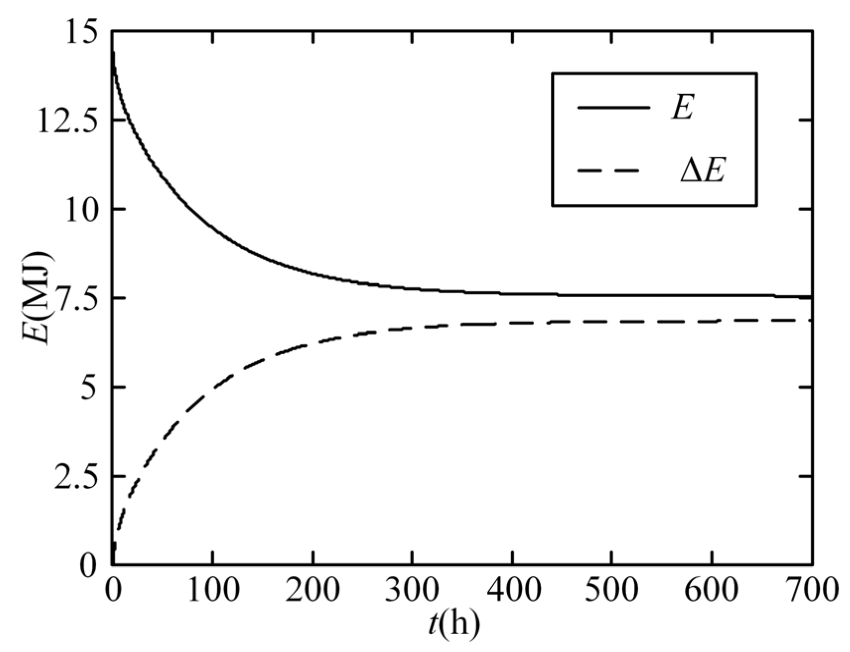
Figure 18 shows the variety of complete exergy and exergy misfortune in the tank with time during the idle condition. It can be found that the total exergy in the tank is gradually reduced with time, while the energy loss grows with time gradually. The thermal disparity in the thermocline decreases as the thermocline thickens. Both the overall exergy loss and the increase in exergy loss eventually slowed down.
5. Conclusions
In this paper, a changed one-layered dimensionless model for the thermocline stockpiling tank is established and its innovative solving method is proposed. Based on the proposed model, the impacts of three unique boundaries on the presentation of the thermocline tank are considered. The characteristic of idle condition is also simulated. Following is a summary of the findings:
- (1)
- In the modified one-dimensional dimensionless model, the heat storage medium’s thermophysical characteristics are regarded as important. At a certain position, it is dependent on the temperature instead of keeping constant. This modified model is closer to reality. Using the proposed adaptive strategy for solving region compartmentalization, the computing time can be reduced.
- (2)
- The thermocline’s thickness rises with time during a charging process. However, it tends to rise more slowly. With the progression of the charging process, the total amount of energy stored in the storage container rises almost linearly.
- (3)
- The degree of thickness of the thermocline reduces from 0.47 m to 0.28 m when the intake velocity increases from 0.0001 m/s to 0.0003 m/s and the productivity of the framework can be increased by increasing the intake velocity.
- (4)
- Expanding the temperature contrast between the hot and cold water from 15 K to 75 K, the thickness of the thermocline increases from 0.29 m to 0.35 m. However, the energy put into the tank is raised. The motion characteristic for the thermocline is unaffected by increasing tank height, although system effectiveness can be improved.
- (5)
- For the idle condition, the thermocline region fills the whole tank about 19 h later under the given conditions and a consistent tank temperature appears about 700 h later.
Author Contributions
Conceptualization, H.J. and L.Z.; methodology, H.J. and W.Z.; investigation, H.J.; resources, H.J.; data curation, L.Z.; writing—original draft preparation, H.J.; writing—review and editing, H.J., L.Z. and W.Z.; visualization, H.J.; supervision, L.Z. and W.Z.; project administration, L.Z.; funding acquisition, W.Z. All authors have read and agreed to the published version of the manuscript.
Funding
This research received no external funding.
Data Availability Statement
Data are contained within the article.
Conflicts of Interest
The authors declare no conflict of interest.
References
- De Rosa, M.; Afanaseva, O.; Fedyukhin, A.V.; Bianco, V. Prospects and characteristics of thermal and electrochemical energy storage systems. J. Energy Storage 2021, 44, 103443. [Google Scholar]
- Cui, S.; He, Q.; Shi, X.; Liu, Y.; Du, D. Dynamic characteristics analysis for energy release process of liquid air energy storage system. Renew. Energy 2021, 180, 744–755. [Google Scholar] [CrossRef]
- Selvakumar, R.D.; Wu, J.; Ding, Y.; Alkaabi, A.K. Melting behavior of an organic phase change material in a square thermal energy storage capsule with an array of wire electrodes. Appl. Therm. Eng. 2023, 228, 120492. [Google Scholar] [CrossRef]
- Guédez, R.; Spelling, J.; Laumert, B.; Fransson, T. Optimization of thermal energy storage integration strategies for peak power production by concentrating solar power plants. Energy Procedia 2014, 49, 1642–1651. [Google Scholar] [CrossRef]
- Khan, M.I.; Asfand, F.; Al-Ghamdi, S.G. Progress in research and technological advancements of thermal energy storage systems for concentrated solar power. J. Energy Storage 2022, 55, 105860. [Google Scholar]
- Votyakov, E.V.; Bonanos, A.M. A perturbation model for stratified thermal energy storage tanks. Int. J. Heat Mass Transf. 2014, 75, 218–223. [Google Scholar] [CrossRef]
- Pacheco, J.E.; Showalter, S.K.; Kolb, W.J. Development of a molten-salt thermocline thermal storage system for parabolic trough plants. J. Sol. Energy Eng. 2002, 124, 153–159. [Google Scholar] [CrossRef]
- Rosen, M.A.; Tang, R.; Dincer, I. Effect of stratification on energy and exergy capacities in thermal storage systems. Int. J. Energy Res. 2004, 28, 177–193. [Google Scholar] [CrossRef]
- Kindi, A.A.; Aunedi, M.; Pantaleo, A.M.; Strbac, G.; Markides, C.N. Thermo-economic assessment of flexible nuclear power plants in future low-carbon electricity systems: Role of thermal energy storage. Energy Convers. Manag. 2022, 258, 115484. [Google Scholar]
- Brumleve, T.D. Sensible heat storage in liquids. In NASA STI/Recon Technical Report N; NASA: Washington, DC, USA, 1974. [Google Scholar]
- Solé, C.; Medrano, M.; Castell, A.; Nogués, M.; Mehling, H.; Cabeza, L.F. Energetic and exergetic analysis of a domestic water tank with phase change material. Int. J. Energy Res. 2008, 32, 204–214. [Google Scholar] [CrossRef]
- Jack, M.W.; Wrobel, J. Thermodynamic optimization of a stratified thermal storage device. Appl. Therm. Eng. 2009, 29, 2344–2349. [Google Scholar] [CrossRef]
- Savicki, D.L.; Vielmo, H.A.; Krenzinger, A. Three-dimensional analysis and investigation of the thermal and hydrodynamic behaviors of cylindrical storage tanks. Renew. Energy 2011, 36, 1364–1373. [Google Scholar] [CrossRef]
- Ievers, S.; Lin, W. Numerical simulation of three-dimensional flow dynamics in a hot water storage tank. Appl. Energy 2009, 86, 2604–2614. [Google Scholar] [CrossRef]
- Nelson, J.E.B.; Balakrishnan, A.R.; Murthy, S.S. Transient analysis of energy storage in a thermally stratified water tank. Int. J. Energy Res. 1998, 22, 867–883. [Google Scholar] [CrossRef]
- Schumann, T.E.W. Heat transfer: A liquid flowing through a porous prism. J. Frankl. Inst. 1929, 208, 405–416. [Google Scholar] [CrossRef]
- Vortmeyer, D.; Schaefer, R.J. Equivalence of one and two-phase models for heat transfer processes in packed beds: One dimensional theory. Chem. Eng. Sci. 1974, 29, 485. [Google Scholar] [CrossRef]
- Bayon, R.; Rojas, E. Simulation of thermocline storage for solar thermal power plants: From dimensionless results to prototypes and real-size tanks. Int. J. Heat Mass Transf. 2013, 60, 713–721. [Google Scholar] [CrossRef]
- Oppel, F.J.; Ghajar, A.J.; Moretti, P.M. A numerical and experimental study of stratified thermal storage. ASHRAE Trans. 1986, 92, 293–309. [Google Scholar]
- Zurigat, Y.H.; Liche, P.R.; Ghajar, A.J. Turbulent mixing correlations for a thermocline thermal storage tank. AICHE Symp. Ser. 1988, 84, 160–168. [Google Scholar]
- Ghaddar, N.K.; Al-Maarafie, A.M. Study of charging of stratified storage tanks with finite wall thickness. Int. J. Energy Res. 1997, 21, 411–427. [Google Scholar] [CrossRef]
- Yoo, H.; Pak, E.T. Theoretical model of the charging process for stratified thermal storage tanks. Sol. Energy 1993, 51, 513–519. [Google Scholar] [CrossRef]
- Davidson, J.H.; Adams, D.A.; Miller, J.A. A coefficient to characterize mixing in solar water storage tanks. J. Sol. Energy Eng. 1994, 116, 94–99. [Google Scholar] [CrossRef]
- Andersen, E.; Furbo, S.; Fan, J. Multilayer fabric stratification pipes for solar tanks. Sol. Energy 2007, 81, 1219–1226. [Google Scholar] [CrossRef]
- Yee, C.K.; Lai, F.C. Effects of a porous manifold on thermal stratification in a liquid storage tank. Sol. Energy 2001, 71, 241–254. [Google Scholar] [CrossRef]
- Castell, A.; Medrano, M.; Sole, C.; Cabeza, L.F. Dimensionless numbers used to characterize stratification in water tanks for discharging at low flow rates. Renew. Energy 2010, 35, 2192–2199. [Google Scholar] [CrossRef]
- Fernández-Seara, J.; Uhía, F.J.; Sieres, J. Experimental analysis of a domestic hot water storage tank. Part II: Dynamic mode of operation. Appl. Therm. Eng. 2007, 27, 137–144. [Google Scholar] [CrossRef]
- Rosen, M.A. The exergy of stratified thermal energy storages. Sol. Energy 2001, 71, 173–185. [Google Scholar] [CrossRef]
- Mosaffa, A.H.; Farshi, L.G.; Ferreira, C.A.I.; Rosen, M.A. Advanced exergy analysis of an air conditioning system incorporating thermal energy storage. Energy 2014, 77, 945–952. [Google Scholar] [CrossRef]
- Han, Y.M.; Wang, R.Z.; Dai, Y.J. Thermal stratification within the water tank. Renew. Sustain. Energy Rev. 2009, 13, 1014–1026. [Google Scholar] [CrossRef]
- Cònsul, R.; Rodríguez, I.; Pérez-Segarra, C.D.; Soria, M. Virtual prototyping of storage tanks by means of three-dimensional CFD and heat transfer numerical simulations. Sol. Energy 2004, 77, 179–191. [Google Scholar] [CrossRef]
- Rosen, M.A.; Dincer, I. Exergy methods for assessing and comparing thermal storage systems. Int. J. Energy Res. 2003, 27, 415–430. [Google Scholar] [CrossRef]
- He, Z.; Wang, X.; Du, X.; Amjad, M.; Yang, L.; Xu, C. Experiments on comparative performance of water thermocline storage tank with and without encapsulated paraffin wax packed bed. Appl. Therm. Eng. 2019, 147, 188–197. [Google Scholar] [CrossRef]
Figure 1.
A diagram of thermocline movement during a typical charging process. (a) The thermocline remains at the tank’s top when the charging process begins. (b) The thermocline moves downward as flow continues. (c) The movement halts when the thermocline touches the tank’s bottom.
Figure 1.
A diagram of thermocline movement during a typical charging process. (a) The thermocline remains at the tank’s top when the charging process begins. (b) The thermocline moves downward as flow continues. (c) The movement halts when the thermocline touches the tank’s bottom.
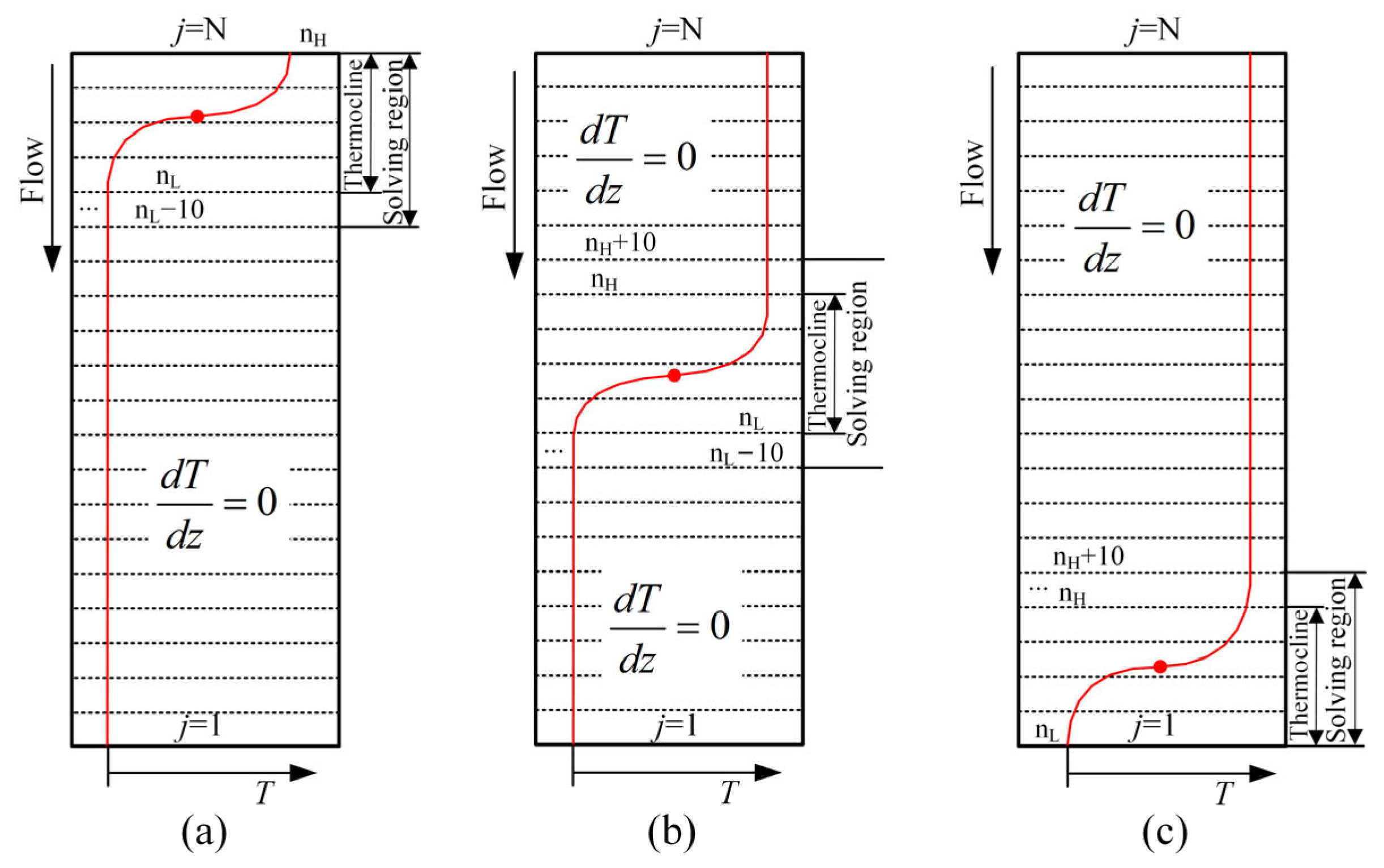
Figure 2.
Temperature changes over time at various tank vertical positions when the tank is being charged [33].
Figure 2.
Temperature changes over time at various tank vertical positions when the tank is being charged [33].
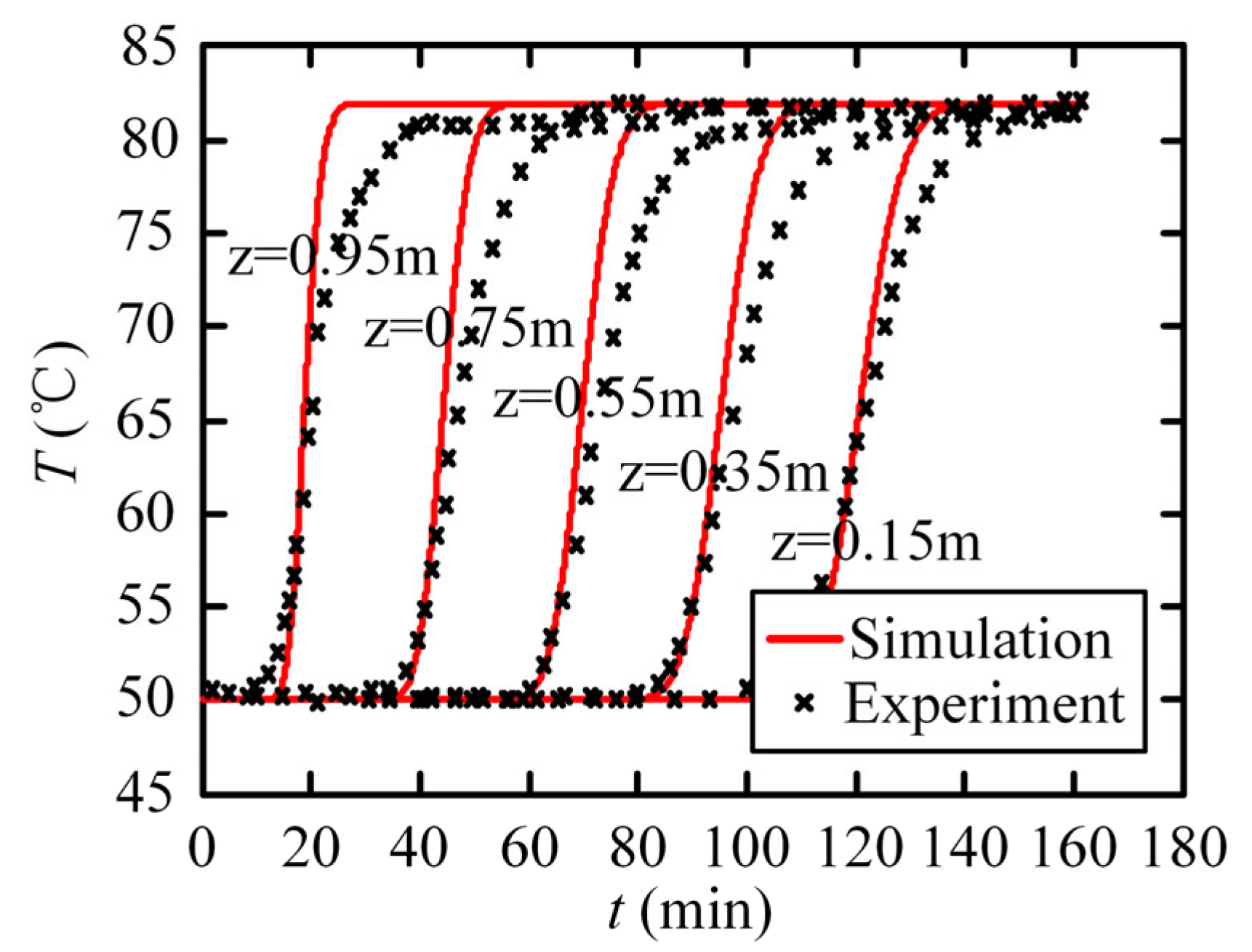
Figure 3.
The temperatures profiles in the tank during a discharge cycle with intervals of 30 min [7].
Figure 3.
The temperatures profiles in the tank during a discharge cycle with intervals of 30 min [7].

Figure 4.
Thermocline thickness fluctuations over time for various inflow velocities.
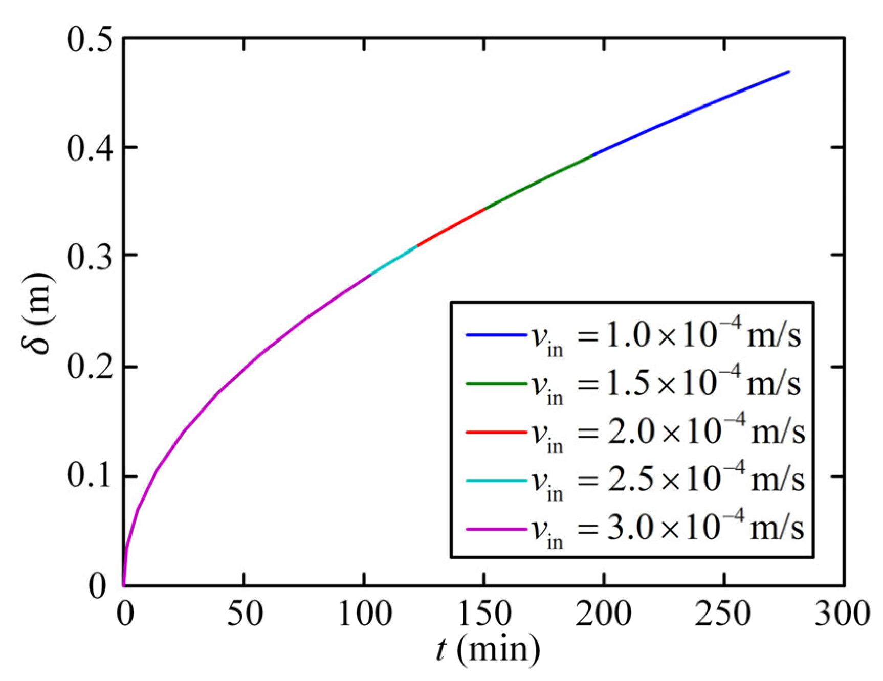
Figure 5.
Efficiency changes depending on inlet velocity.
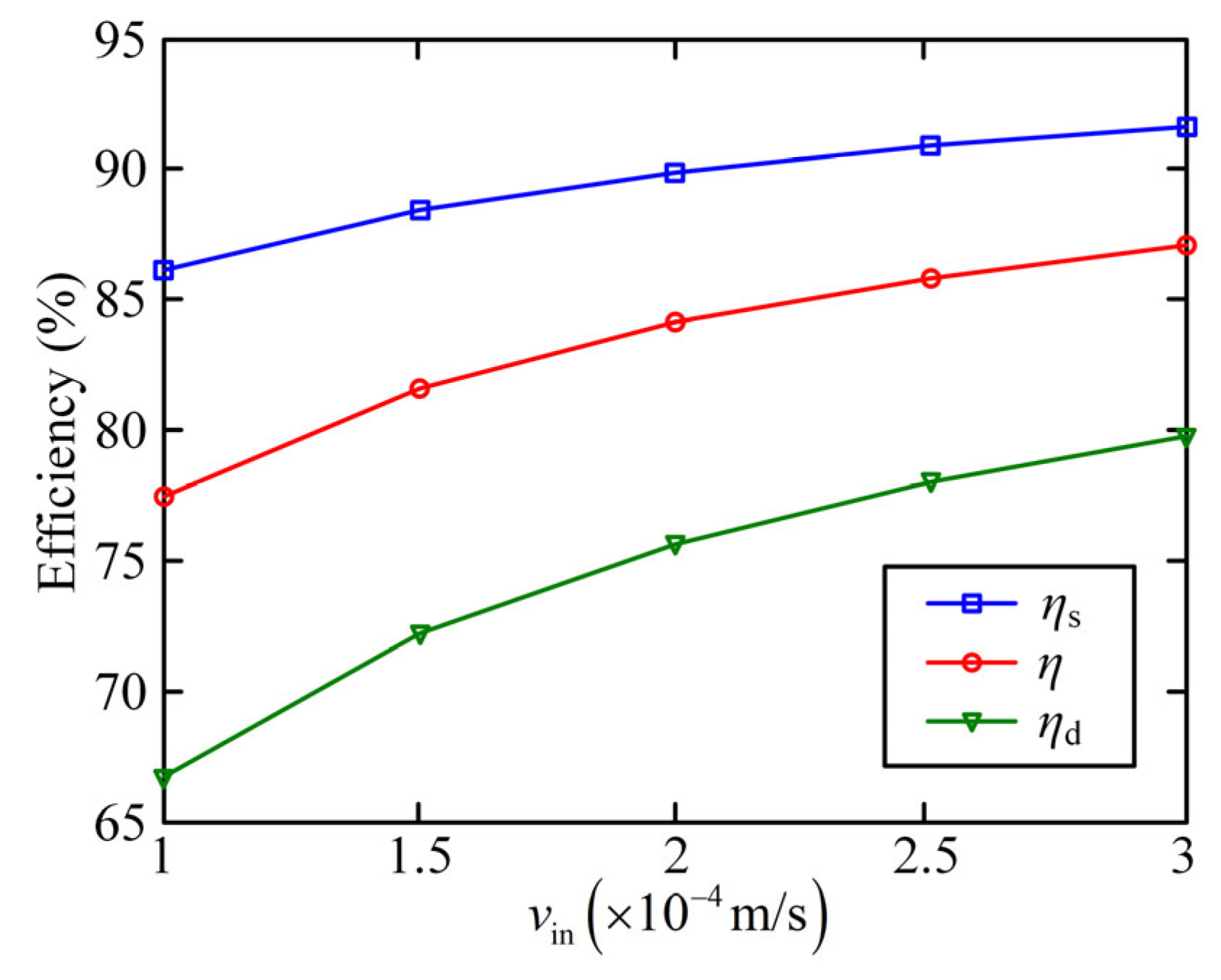
Figure 6.
Total energy change over time within the reservoir based on different inflow velocities.
Figure 7.
The change in energy loss over time within the reservoir at various inlet velocities.

Figure 8.
Variation of thermocline thickness with time for different inlet temperatures.
Figure 9.
Efficiency variation with inlet temperatures.
Figure 10.
Exergy variation over time for various intake temperatures.
Figure 11.
Variation of exergy loss with time for different inlet temperatures.

Figure 12.
Variation of thermocline thickness with time for different tank height.
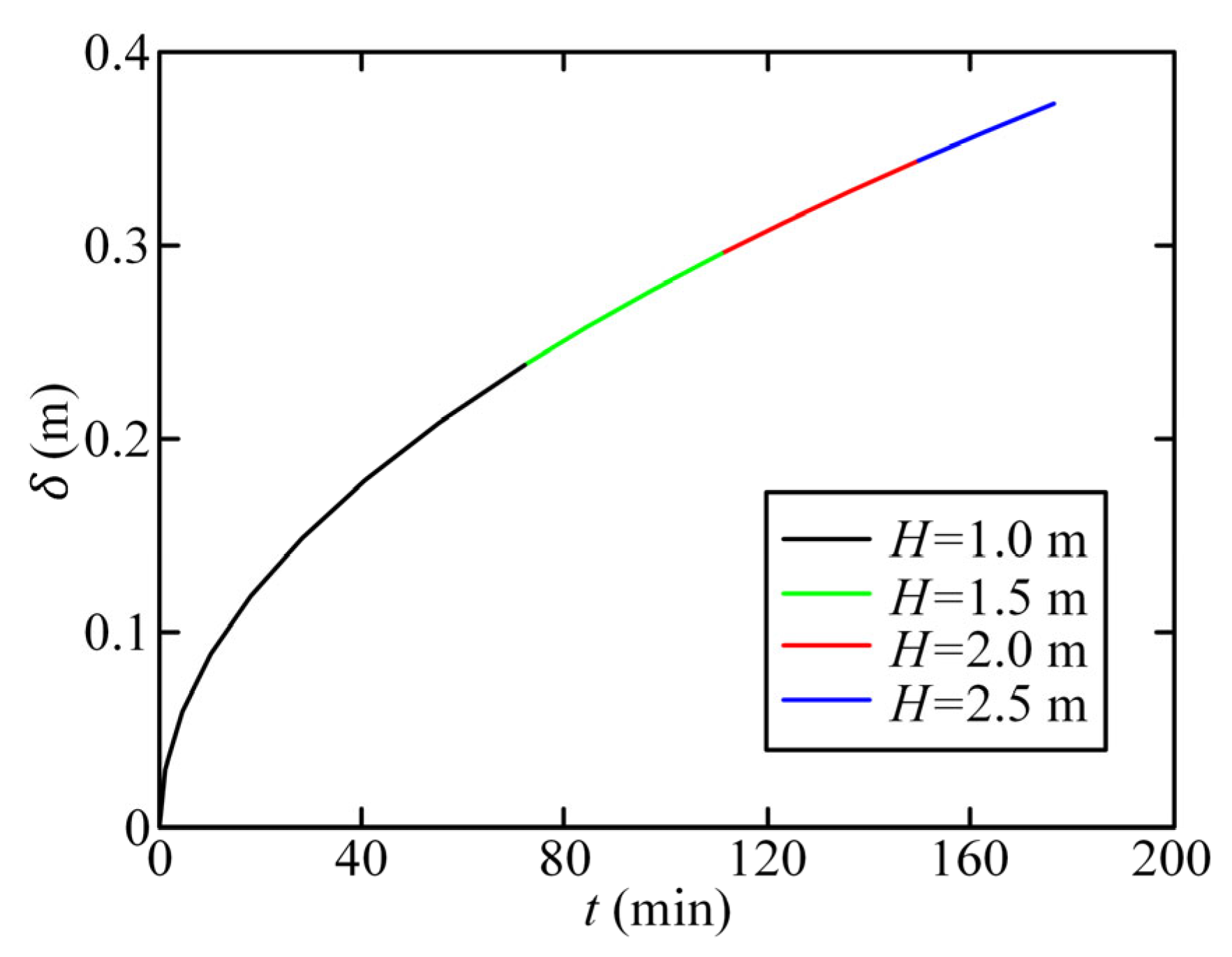
Figure 13.
Variations of efficiency with tank heights.

Figure 14.
Exergy changes with time at various tank heights.
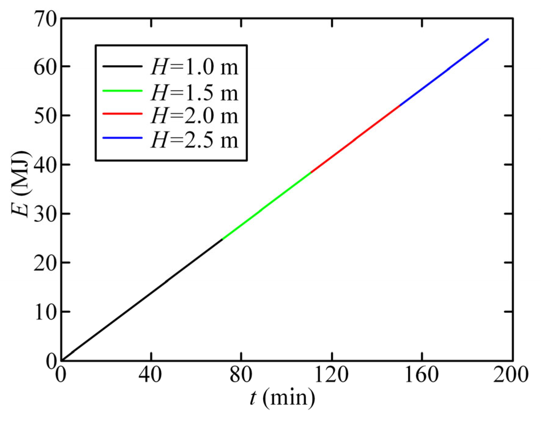
Figure 15.
Exergy loss varies with time at various intake temperatures.
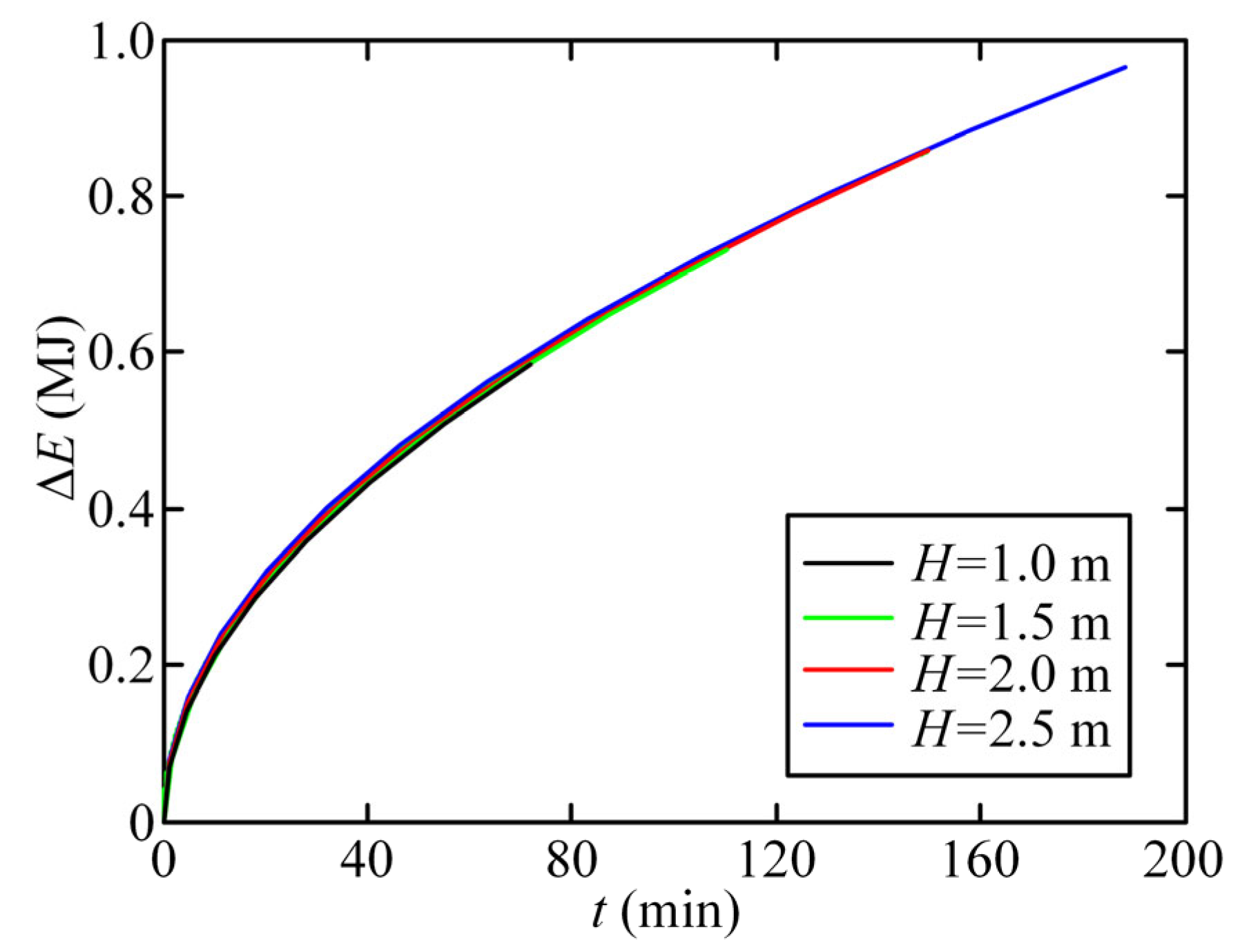
Figure 16.
Temperature distribution inside the storage container during the idle condition.
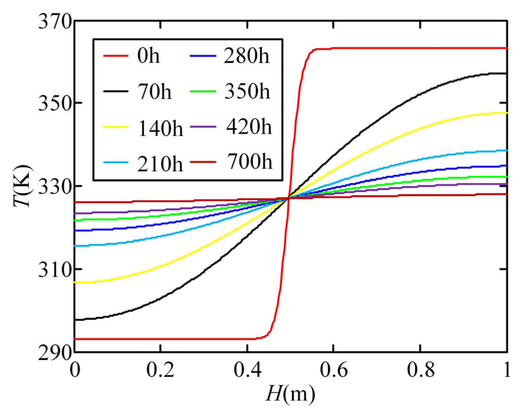
Figure 17.
Thermocline thickness varies throughout time. during the idle condition.

Figure 18.
Variation of total Exergy leakage and overall power in the storage container with time during idle condition.
Figure 18.
Variation of total Exergy leakage and overall power in the storage container with time during idle condition.

Table 1.
Principal traits and thermocline tank design variables employed in the model validation.
| Design Criteria | Thermocline Storage Tank Type | |
|---|---|---|
| Water Tank | Sandia Lab Prototype | |
| Height (m) | 1.1 | 6 |
| Diameter (m) | 0.9 | 3 |
| Velocity (m/s) | 1.31 × 10⁻⁴ | 4.186 × 10⁻⁴ |
| Tmax (°C) | 83 | 390 |
| Tmin (°C) | 50 | 290 |
| Porosity, ε | 1 | 0.22 |
| Storage medium | Water | Rock/sand and eu-NaNO3/KNO3 |
Table 2.
Boundary conditions and related physical property parameters.
| Parameter | Symbol | Unit | Reference Value |
| Temperature sensitivity | k | W/(m·K) | Equation (24) |
| Specific heat capacity | Cp | J/(kg·K) | Equation (25) |
| Density | ρ | kg/m3 | Equation (26) |
| Hot water temperature | Tmax | K | 363.15 |
| Cold water temperature | Tmin | K | 293.15 |
| Prevailing temperature | T0 | K | 293.15 |
| Reference temperature | Tin | K | 363.15 |
| Reference tank height | H | m | 2 |
| Cross-sectional area | A | m2 | 1 |
| Reference velocity | vin | m/s | 2 × 10⁻⁴ |
Disclaimer/Publisher’s Note: The statements, opinions and data contained in all publications are solely those of the individual author(s) and contributor(s) and not of MDPI and/or the editor(s). MDPI and/or the editor(s) disclaim responsibility for any injury to people or property resulting from any ideas, methods, instructions or products referred to in the content. |
© 2023 by the authors. Licensee MDPI, Basel, Switzerland. This article is an open access article distributed under the terms and conditions of the Creative Commons Attribution (CC BY) license (https://creativecommons.org/licenses/by/4.0/).
Share and Cite
MDPI and ACS Style
Ju, H.; Zheng, L.; Zhong, W. Numerical Research on Thermodynamic Properties of a Thermocline in Thermal Energy Storage Tank Based on Modified One-Dimensional Dimensionless Model. Energies 2023, 16, 7499. https://doi.org/10.3390/en16227499
AMA Style
Ju H, Zheng L, Zhong W. Numerical Research on Thermodynamic Properties of a Thermocline in Thermal Energy Storage Tank Based on Modified One-Dimensional Dimensionless Model. Energies. 2023; 16(22):7499. https://doi.org/10.3390/en16227499
Chicago/Turabian StyleJu, Haoran, Lijun Zheng, and Wei Zhong. 2023. "Numerical Research on Thermodynamic Properties of a Thermocline in Thermal Energy Storage Tank Based on Modified One-Dimensional Dimensionless Model" Energies 16, no. 22: 7499. https://doi.org/10.3390/en16227499
Note that from the first issue of 2016, this journal uses article numbers instead of page numbers. See further details here.