


Research on Optimum Charging Current Profile with Multi-Stage Constant Current Based on Bio-Inspired Optimization Algorithms for Lithium-Ion Batteries †

Department of Marine Engineering, National Taiwan Ocean University (NTOU), Keelung 20224, Taiwan
*
Author to whom correspondence should be addressed.
†
This paper is a rewritten and extended article recommended to Energies after presented at the 6th IEEE International Conference on Knowledge Innovation and Invention 2023 (ICKII 2023) on 21–23 August 2023 in Hokkaido, Japan. (Paper no.: K230105).
Energies 2023, 16(22), 7641; https://doi.org/10.3390/en16227641
Submission received: 10 October 2023
/
Revised: 2 November 2023
/
Accepted: 15 November 2023
/
Published: 17 November 2023
(This article belongs to the Topic Application of IoT on Manufacturing, Communication and Engineering)
Abstract
:Compared with the conventional constant-current constant-voltage (CC-CV) charging method, the multi-stage constant-current (MSCC) charging method offers advantages such as rapid charging speed and high charging efficiency. However, MSCC must find the optimal charging current profile (OCCP) in order to achieve the aforementioned benefits. Hence, in this paper, five bio-inspired optimization algorithms (BIOAs), including particle swarm optimization (PSO), modified PSO (MPSO), grey wolf optimization (GWO), modified GWO (MGWO), and the jellyfish search algorithm (JSA), are applied to solve the problem of searching for the OCCP of the MSCC. The best solution-finding procedure is run on the MATLAB platform developed based on minimizing the objective function of combining charging time (CT) and energy loss (EL) with a proportional weight. Without requiring numerous and time-consuming actual charge-and-discharge experiments, a wide range of searches can be quickly achieved only through the battery equivalent circuit model (ECM) established. The theoretical derivation and correctness are confirmed via the simulation and experimental results, which demonstrate that the OCCPs obtained by using the devised charging strategies possess the shortest CT and the best charging efficiency (CE), and among them, MPSO has the best fitness value (FV). Compared with the traditional CC-CV method, the experimental results show that the maximum improvement rates (IRs) of the studied approaches in terms of six charging performance evaluation indicators (CPEIs), including CT, charging capacity (CHC), CE, charging energy (CWh), average temperature rise (ATR), and FV, are 21.10%, 0.40%, 0.24%, 2.85%, 18.86%, and 68.99%, respectively. Furthermore, according to the comprehensive evaluation with CPEIs, the top three with the best overall performance are the JSA, MPSO, and GWO methods, respectively.
1. Introduction
With the fast development of portable electronic devices, renewable energy systems, and electric vehicles (EVs), as well as advancements in battery-related technologies, lithium-ion batteries (LiBs) have garnered significant attention as a highly promising option for secondary batteries. They possess numerous advantages, including high energy density, compact size, long cycle life, high discharge current tolerance, and the absence of memory effects. As a result, many high-power energy storage systems have begun to focus on the research and development of high-capacity LiBs [1,2,3]. Charging techniques play a crucial role in the performance and lifespan of LiBs. Factors directly affected include the following: (1) Charging time: the charging technique employed dominates the time required to fully charge LiBs. Efficient charging algorithms can optimize the charging process and reduce the overall CT. (2) Charging efficiency: the charging technique influences the efficiency of energy transfer during the charging process. Higher CE means less energy loss and more effective utilization of the charging power. (3) Charging temperature rise (TR): proper charging techniques help mitigate the TR of LiBs during charging. Excessive TR can result in thermal stress, accelerated degradation, and safety concerns. (4) Longevity: the chosen charging technique affects the number of charge–discharge cycles that the LiB can endure before its capacity significantly degrades. (5) State of charge (SOC): charging the battery with sufficient SOC and accurately estimating the remaining capacity can help the system make comprehensive decisions and improve system safety [4]. (6) Micro-health parameters: the micro-health parameters represent the performance of active material and electrolytes inside the battery, and the changes in the micro-health parameters represent the battery’s internal health state [5]. Optimal charging techniques can extend the cycle life of the battery and ensure its performance retention over a longer period. That is, charging techniques have a significant impact on various aspects of LiB performance. Using appropriate charging techniques can optimize these factors and enhance the overall performance and lifetime of the battery. On the other hand, LiBs are susceptible to factors such as overcharging, over-discharging, and environmental temperature, leading charging technologies that consider the impact of these factors to become a future research trend [6,7,8]. Furthermore, in response to the development of fast charging for EVs, high-current charging can lead to a high TR, low CE, and short lifespan. Among these factors, TR is particularly critical for batteries. A higher TR during charging indicates greater energy loss and raises safety concerns.
Currently, numerous researchers are still putting forward different perspectives and conducting investigations on various charging methods to address different charging issues. Their goals often revolve around shortening charging time, reducing charging temperature rise, and improving charging efficiency. Currently, the most commonly adopted charging method is the CC-CV method. This method involves initially charging the LiB with a CC, causing the battery voltage to increase. When the battery voltage reaches the upper limit voltage (e.g., 4.2 V for LiB), the charging mode switches to CV. During the CV phase, the battery is charged at the limit voltage while the charging current gradually decreases until it reaches the preset minimal value (e.g., 0.02 C), at which point the charging is terminated. This method combines the advantages of both CC and CV methods and is relatively simple and easy to implement. However, this method requires a longer CT during the CV mode, resulting in an overall longer CT and potentially shorter cycle life. Accordingly, many studies proposed in the literature aim to explore new charging algorithms, charging control strategies, and charging system designs to improve charging effectiveness while ensuring safety and battery lifetime.
In the derivative CC-CV charging methods, a dual-loop control strategy based on battery voltage was proposed in [9] to achieve a charge similar to CC-CV. It does not require a current sensor, making it simpler and more cost-effective. A boost-type CC-CV method is proposed in [10]; it starts with a voltage higher than the battery rated voltage and then switches to the standard CC-CV after the boost voltage period. This approach can reduce the CT compared with the CC-CV, but it requires the battery to be fully discharged before charging. A gray prediction control was adopted in [11], while a fuzzy controller was utilized in [12] to achieve higher charging capacity in CV mode. A current pump battery charger was proposed in [13]. The current pump was used in CC mode, and the pulse current was adopted in CV mode. Experimental results show that the CE is higher and the overall CT is comparable to the CC-CV. Ref. [14] proposed a closed-loop constant-temperature constant-voltage (CT-CV) charging method, which realizes constant temperature charging through a PID controller.
In terms of optimal charging methods based on battery models, ref. [15] considers a second-order RC model for LiBs and incorporates the model predictive control to minimize the evaluation function using pulse magnitude modulation and pulse width modulation. In order to improve the charging performances, ref. [16] inputs the TR and TR change rate into the fuzzy controller to deduce the desired charging current value. The experimental results show that the CE and TR can be improved. Ref. [17] raises an optimization method based on the electrochemical model of health, TR, and aging to make a trade-off between CT and aging speed. The MaxLifeTM charging technology proposed in [18] estimates the electrochemical parameters via the construction of aging and electrochemical models. During the charging process, it can dynamically adjust the proper charging voltage and current through control mechanisms. Compared with the CC-CV, this approach features a higher TR; however, it effectively mitigates lithium dendrite formation and prevents battery expansion, resulting in longevity improvement. In the context of research related to pulse charging methods, the highest charging current can be achieved by altering the pulse frequency [19] or adjusting the duty cycle of the pulses [20]. In addition, refs. [21,22] explore various variations in charging methods by modifying the current magnitude, pulse width, and resting period. In [23], an adaptive pulse adjustment is raised to improve charging speed and charging efficiency. Under the proper parameter setting and operating conditions, the charging techniques mentioned above can effectively improve the charging performance. However, these methods have high complexity in implementation and need the use of costly digital controllers.
The MSCC charging method applies different levels of current to charge. In the literature, transition criteria of the current level are mainly divided into two categories: battery terminal voltage and remaining capacity. Refs. [24,25,26] employ terminal voltage as the transition criterion of charge current based on the constraint that the current in the subsequent stage must be less than that of the previous stage. If the battery could not be fully charged, it is a problem for the voltage-based transition. To cope with this issue, a CV mode is often added after the final stage charge [27,28]. Although this way can achieve the full charge, it comes at the cost of longer CT and lower CE. Refs. [29,30,31,32] adopt the SOC as the current transition criterion. In this criterion, the current value in each stage is not subject to the aforementioned restriction. Compared with the CC-CV method, the SOC-based transition method can reduce CT and have higher CE than the pulse charging method. In recent years, studies on searching the OCCP of MSCC using optimization algorithms (OAs), such as the ant colony system (ACS) [24], Bayesian optimization [28], genetic algorithm (GA) [32], PSO [33], cuckoo optimization algorithm (COA) [34], GWO [35], etc., have been proposed. The OA can improve the search capability for multi-objective optimal solutions and simultaneously consider multiple charging performance indicators to significantly improve the charging performance as compared with the CC-CV. However, these methods require experimental verification for candidate charging patterns, which requires a lot of experimental time and results in a significant increase in the time and cost of finding the optimal solution. In addition, based on the simplified ECM, ref. [36] proposed a formula calculation method (dubbed FC method in this paper) to determine the OCCP of MSCC. A set of simple formulas are derived to calculate each stage’s current value. In comparison with the aforementioned methods, this approach does not require extensive experiments and time costs. However, it is only dedicated to improving the CT and does not take the EL or TR into account.
The MSCC charging method primarily evaluates the contribution of the charge current in each stage to the total CHC, CT, and EL. Accordingly, finding the OCCP is crucial for MSCC. Based on the battery ECM and five BIOAs, i.e., PSO, modified PSO [37], GWO, modified GWO [38], and JSA [39], this paper aims to search the OCCP of the MSCC method with an objective function that simultaneously minimizes the combination of charging EL and CT. Firstly, an ECM is established by the analysis of electrochemical impedance spectroscopy (EIS). Then, mathematical expressions for CPEIs are derived to formulate the optimization problem studied. Finally, a MATLAB-based computation platform, consisting of the ECM, CPEI calculation formulas, and BIOAs, is formed to discover the OCCP that features the best fitness value. The main contributions of this paper include the following: (1) Without the need for numerous and long-lasting experimental processes, the OCCP search can be quickly achieved only through the ECM-based computation platform established. (2) The OCCP searching procedure is completed based on the consideration of multi-objective optimization. (3) The JSA applied to the OCCP search of LiBs is first proposed. (4) A comprehensive evaluation of the studied BIOA-based method is performed to make the recommendation for charging method adoption. (5) The proposed charging strategy could be extended to other types of batteries. The rest of this paper is organized as follows. The basic philosophy of the proposed charging strategy, including the battery ECM and parameter measurement, mathematical derivation of the presented MSCC charging method, formulation of the optimization problem, and the definition of the fitness function, is described in Section 2 in detail. Section 3 provides a review of the BIOAs, their operating mechanisms, and the flowchart applied to the studied method. The results of the simulation and experiment are given in Section 4 to demonstrate the validity and effectiveness. Comparisons with the conventional methods are also performed to emphasize performance improvement. Finally, Section 5 concludes this paper.
2. Philosophy of the Proposed Charging Strategy
To facilitate the analysis of the complicated electrochemical behavior, this section first introduces the ECM of the LiB selected. Next, the identification of the parameters in the ECM through the analysis of the AC impedance is depicted, and then the fitted ECM is applied to derive the mathematical formulas of the MSCC charging method. Finally, the BIOAs, integrated with the objective function of simultaneously achieving the reduction in CT and EL, are applied to find the optimal multi-stage charging current patterns.
2.1. Equivalent Circuit Model and Parameter Measurement
Building an accurate battery ECM is helpful for theoretical derivation, analysis, and experimental verification. During the charging or discharging process, the battery output voltage varies over time due to the influence of internal electrochemical reactions. Figure 1 shows the first-order Thévenin’s ECM of the battery adopted in this study, which consists of the battery equivalent capacitance Ceq, polarization resistance Rp, capacitance Cp, and internal resistor Ro. This model has the advantages of adequate accuracy and low computational burden. Rp and Cp represent the charge transfer and diffusion process between the electrode and the electrolyte. The dynamic response of the battery can be described by the parallel Rp and Cp. Through this ECM, the CT, EL, and charging capacity of the studied MSCC method can be derived. If the battery works at a specific temperature, the Rp, Cp, and Ro are all related to the SOC, and this ECM can characterize the behavior of dynamic and steady states with acceptable accuracy during the charging and discharging processes.
In this work, the dominant parameters (Rp, Cp, and Ro) shown in the ECM were identified by using the AC impedance analysis (AIA) method. Figure 2a shows the flowchart of the AIA experiment. The AC impedance and OCV are measured every 1% SOC interval in this paper. First, fully charge the battery (100% SOC) with CC-CV and rest for 3 h. Then, execute the EIS testing subroutine to obtain the ECM model parameters. Next, discharge with 0.1 C CC for 6 min (about 1% SOC), rest for 3 h, and then measure the OCV. The entire experiment is conducted until the SOC drops to 0%. Figure 2b shows the subroutine of the electrochemical impedance spectroscopy (EIS) testing. The EIS testing involves perturbing the battery using a small-amplitude AC sinewave signal with variable frequency. The amplitude of the testing sinewave voltage is 10 mV, and the testing frequency range is set from 0.1 Hz to 100 kHz with intervals of 6 dB. The AC impedance of a battery has a corresponding relationship with the remaining capacity and can be characterized by the Nyquist plot. This paper considers the accuracy of the ECM and the time required for testing, and a precision of 1% SOC is used for AC impedance analysis. Then, the measured AC impedance values under different SOCs are utilized to fit the desired battery model and identify its corresponding parameters. The Panasonic NCR18650GA LiB was studied in this paper. The test and analysis platform formed by Bio-logic SP-100 Potentiostat with EC-Lab V11.40 software from BioLogic was used to perform the AIA. When the battery is working at a specific temperature, the model parameters are a function of SOC. Figure 3a,b show the measured curves of the open-circuit voltage (OCV), Rp, and Ro, where Req is the equivalent internal resistance (EIR) that is defined as Req = Rp + Ro. In order to easily calculate the Req under different SOCs when deriving the total CT and EL, the curve fitting of Req by using the Gaussian summation function model is conducted, and the result is
where the coefficients of [a1, b1, c1, a2, b2, c2, a3, b3, c3, a4, b4, c4, a5, b5, c5, a6, b6, c6] are equal to [0.09555, −0.06814, 0.1023, 1.322 × 10⁵, 6.617, 1.488, 0.1348, −0.184, 0.5725, 0.09618, 0.6407, 0.5104, 0.002261, 0.7916, 0.139, −6.518 × 10⁻⁵, 0.7956, 0.03881].
Figure 1.
The battery ECM adopted in this study.

Figure 2.
(a) Flowchart of the AIA experiment; (b) subroutine of EIS testing.

Figure 3.
Model parameter measurement: (a) OCV-SOC curve; (b) equivalent internal resistance.

2.2. Mathematical Derivation of the Proposed Charging Method
As shown in Figure 1, the VCeq, VCp, VRp, VRo, and VT represent battery internal voltage (or OCV), voltages across Cp, Rp, and Ro, and the battery terminal voltage, respectively. According to the Kirchhoff law, the VT can be expressed by
Figure 4 illustrates the schematic waveforms of battery voltage, current, and SOC charged by using a typical MSCC method. Where n is the stage number, VCeq,1 is the initial voltage of the SOC at 0%. The study concluded in [27] indicates that increasing the number of current stages can effectively reduce charging time. However, beyond the fifth stage, the benefits are insignificant, and the implemented cost and complexity will be increased substantially. Therefore, the five-stage CC is chosen in this paper. From Figure 4, the electricity charged into the battery at each stage can be expressed as
where In−1 is the charging current of the previous stage, and ∆Vn is the difference between the OCV of each stage and that at the previous stage. Consequently, the CT (∆tn) required during one charging stage can be estimated by
For the duration of the CC charge, the impedance of Cp is much greater than Rp, and then the current flowing through Rp is approximate to the charging current (i.e., IRp ≈ Icharge). Consequently, the internal voltage VCeq,n for each stage can be determined by
where Vcut-off is the cut-off voltage at each current transition point, and Icharge,n is the charging current of each stage. Accordingly, the ΔVn for each stage can be derived by
In addition, in order to charge the battery to 100% SOC, the current value of the fifth stage can be designed by
where VCeq,5 is the internal voltage at full charge. Hence, the total CT (CTtotal) can be determined by
Finally, the total EL (ELtotal) during the charging period depends on the current value of each stage and the EIR values under different SOC conditions. It can be computed by
2.3. Formulation of Optimization Problem
Before applying optimization algorithms to find the best solution, it is necessary to define the optimization objectives and design the objective function accordingly. The objective function is used to calculate the FV of each particle and evaluate the optimization result. This study solves the OCCP simultaneously taking two different physical quantities of the charging CT and EL into account. In which the CT and EL are closely related to the charging current of each stage. As shown in Figure 5, based on the specifications of the studied battery and the requirements for safety, the CC-CV with the charging current range from 1.5 C to 0.5 C with a 0.1 C step is inputted into the ECM built in the developed MATLAB platform to calculate the CTtotal and ELtotal under different C-rate charging points to find the range of feasible solution space for the studied optimization problem. From Figure 5, it can be observed that the ideal solution is located at the position that has the shortest CT (CTmin) and minimal EL (ELmin). Thereby, the linear distance (d) between the solution of the current operating point (CTcop, ELcop) and the ideal optimal solution (CTmin, ELmin) is adopted as the fitness-value function fFV(·) to evaluate whether the operating point is the best solution or not. It can be expressed by
where are the charging current values. Accordingly, the objective function and constraints of the studied optimal problem can be formulated as
where stands for the set of all feasible charging patterns. Since (11) contains two different physical quantities, the maximal and minimal values of the CT and EL are used to normalize the two parameters to ensure the consistency of the benchmark values for the target parameters. In addition, to appropriately balance the significance of the two target CPEIs, a weighting coefficient σ is introduced into the objective function. The constraints of the optimization problem include that the CT and EL are limited to the maximum and minimum values allowed by the feasible solution space. In order to alleviate the chemical reaction stress, the charging current value of the present stage should not be greater than that of the preceding stage. In addition, the current (In) and the transition voltage (VCeq,n) of each stage must not exceed the allowable maximum values, Imax and Vmax, recommended by the battery specification. In this paper, Imax is 3.3 A, and Vmax equals 4.2 V.
3. Bio-Inspired Optimization Algorithms for OCCP Searching
3.1. Overview of BIOAs Studied
Searching for the OCCP for a rechargeable battery can be regarded as a combinatorial optimization problem. Such a problem is hard to solve by using traditional methods. One possible way to obtain the OCCP is to try every combination of the charging current value. However, this way of exhaustive search is time-consuming and not economical for engineers to do so. The BIOA-based optimization techniques have been successfully applied to various research and applications. Hence, this study first establishes an accurate battery ECM through the EIS analysis, and then the objective function that simultaneously considers the minimization of charging EL and CT is derived based on the ECM; finally, combining the ECM with the BIOA method, a computation platform is established on MATLAB to search for the OCCP of the MSCC. In this way, without the need for numerous and time-consuming actual charge-and-discharge experiments, only through the battery ECM-based computation platform, a wide range of searches based on the BIOA approaches to quickly find the OCCP can be achieved.
3.1.1. Modified Particle Swarm Optimization
Particle swarm optimization [37] is a metaheuristic optimization algorithm that draws inspiration from the collective foraging behavior of a flock of birds or fish. Figure 6 shows an update concept of a particle in PSO searching. Particles are used to represent potential solutions. Each particle possesses a fitness value and a corresponding position. The particles continuously adjust their velocities and positions in order to explore the search space and locate the optimal solution. This update process is influenced by both the particle’s own experiences and the experience of the swarm. Initially, the particles are randomly initialized within the solution space, and their positions and velocities are subsequently updated iteratively based on the following two formulas:
For particle q, and are positions of the (k + 1)th and kth iterations in the dth dimension, respectively; and denote velocities of the (k + 1)th and kth iterations in the dth dimension, respectively. w(k) is inertia weight. The c1 and c2 are the cognitive and social learning factors, respectively. ℜ1 and ℜ2 are two random numbers in the interval of [0, 1], respectively. is the location with the best global FV. is the location at which the particle q had the best FV. During each iteration, the particles will modify their convergence speed and update their individual velocity and position by simultaneously taking both experiences of the individual particle (Pbest,q) and the collective particle (Gbest) into account. This iterative process persists until termination conditions, such as reaching the maximum number of iterations or discovering the global optimal FV, are met. In the velocity update Equation (12), since w, c1, and c2 dominate the particle global search capability and local convergence quality, as a result, the inertia weight with a linear decrease was proposed in [33] to improve the problem of poor global exploration and local exploitation capabilities caused by improper weight settings. However, in this linear decrease way, if the tuning value between the three parameters in (12) is not properly matched, the update speed becomes slower, causing the particle search speed to slow down. Once the particle is trapped in the local optimal solution, it may not have enough momentum to escape due to the velocity attenuation.
In order to enhance the global and local search abilities, modified PSO is studied in this paper. In addition to utilizing the cognitive and social models of individual particles in traditional PSO, MPSO adds a new mode called other particles’ best experience (OPBE) to guide the swarm in locating the best solution. The OPBE mode selects a random particle Pbest,ap as the exchange learning experience for the current particle among different individuals. The learning factor c3 in this mode is chosen to be linearly decreasing, from c3,max to c3,min, as the iteration number increases. Adjusting these two parameters can make the algorithm more flexible and applicable to various optimization problems. Therefore, this algorithm enables each particle to search more efficiently and quickly for the global best solution or a solution closer to the global best in the complex solution space. The complete formula of MPSO can be expressed as
The learning factor c3(k) can be denoted by
where c3,max and c3,min are the maximal and minimal values of the c3. The iter and itermax stand for the number of current iterations and the maximum iteration number.
3.1.2. Modified Grey Wolf Optimization
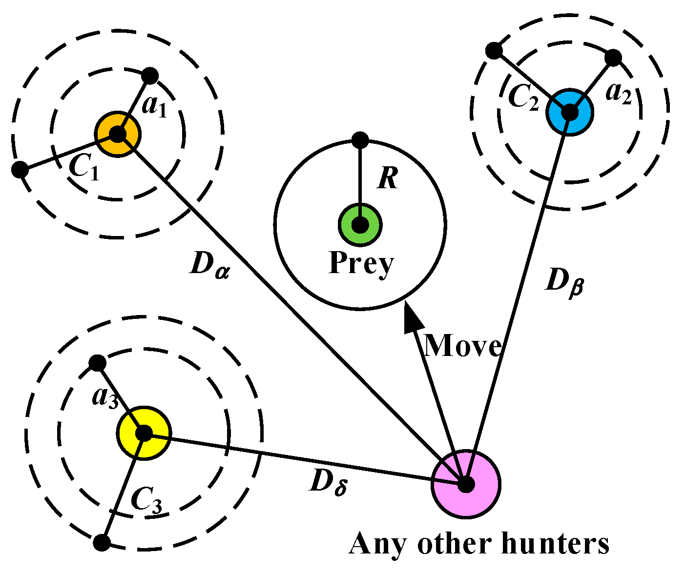
The grey wolf optimizer [38] is a computational method that draws inspiration from the hunting behavior of a pack of grey wolves. Figure 7 depicts the mechanism of the gray wolf position update. The algorithm commences by yielding a model based on random initial solution generation and subsequently identifies the three most optimal solutions within the wolf pack, referred to as α, β, and δ. Afterward, utilizing the positions of these three superior solutions and employing vector coefficients and , the expected forward positions for each solution are sequentially updated. Ultimately, the three anticipated positions are combined and averaged to yield the new position for each grey wolf. The mathematical formulation for updating the positions of the grey wolves is given by
where is the gray wolf position vector. The determination of vector coefficients and can be derived by
where and are random variables in the interval of [0, 1]; is a vector coefficient that decreases from 2 to 0 with each iteration, which can be calculated by
In addition, is a random number between −2 and 2. When > 1, it represents global exploration, and when < 1, it indicates local exploitation. is a random number between 0 and 2, which affects the distance between the target wolf and each wolf, and it helps to avoid falling into local optima.
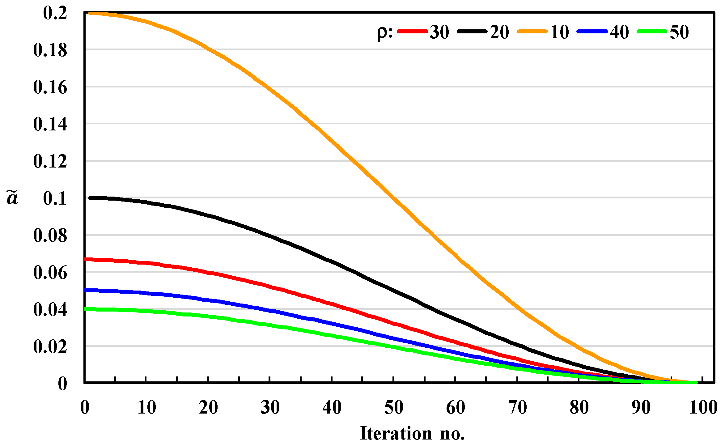
In (21), the value of affects the overall system search speed. In conventional GWO, it decreases linearly to balance the search time between global exploration and local exploitation. However, if the convergence speed is too fast, the search results will easily fall into the local optimal solution, and the search accuracy will be poor. To address this issue, a modified GWO algorithm is studied. Equation (22) is introduced in this paper to change the range of with the computation of the cosine function and adjust the speed of exploration and exploitation. In addition, the π is conducted to capture the descending curve so that the decreases in a cosine curve as the number of iterations increases, which is beneficial to increase the global exploration time. Adding 1 to the numerator term of (22) can make the curve minimal value zero. The value of ρ in the denominator term will further affect the range of and the search time. The curves of under different ρ values are plotted in Figure 8. From Figure 8, it can be observed that the variation in is the same as the traditional GWO when ρ is one and will decrease from 2 to 0 with the iterative process. Compared with traditional GWO, the smaller the ρ is, the larger the is. This helps to maintain the range of and extend the global searching time. In addition, the larger the ρ, the higher the search accuracy, which makes the global search time longer, and the range of is reduced. However, if the selection of ρ is too large, the search range of will be too small, which results in the inability to discover the optimal solution. As a result, choosing an appropriate ρ can effectively increase the global exploration time and make the search results more accurate and the system more stable.
3.1.3. Jellyfish Search Algorithm
The jellyfish search algorithm [39] is inspired by the optimal technology of the jellyfish movement and foraging behavior in the ocean. Figure 9 shows an imitation of an ocean current, a jellyfish swarm, and time control. The movement behavior of jellyfish is mainly affected by the direction of the ocean current, jellyfish swarm, and time control mechanism:
- Ocean current: Ocean currents are rich in nutrients, which make it easy for jellyfish to move along with the currents. The direction of the ocean current, , is determined by the average vector between the position X of all jellyfish and the current optimal position of the jellyfish, . The direction of the ocean current and the position update of the ith jellyfish moving with the ocean current can be respectively expressed by
Figure 9.
Imitation of ocean current, jellyfish swarm, and time control.

- Jellyfish swarm movement: There are two types of jellyfish swarm movements, passive movement (type A) and active movement (type B). When a jellyfish swarm first forms, most jellyfish explore by passive movement. But as time goes by, more and more jellyfish are showing active movement for exploration. Type A movement swarms move by circling around their own position, and the corresponding position update of each jellyfish can be denoted by
- Time control mechanism (TCM): TCM is introduced to control the ratio between the movement of jellyfish following the ocean current and that within the jellyfish swarm. The TCM includes a time control function c(t) and a constant Co (the Co is set to 0.5 in this study). The c(t) is a random value that fluctuates between 0 and 1 over time, and it can be derived by
If c(t) ≥ Co, the movement of jellyfish follows the ocean current; if c(t) < Co, the jellyfish moves within the jellyfish swarm. When moving within the jellyfish swarm, if rand(0, 1) > (1 − c(t)), the jellyfish explores with passive movement; otherwise, it explores with active movement.
3.2. Procedure for OCCP Searching
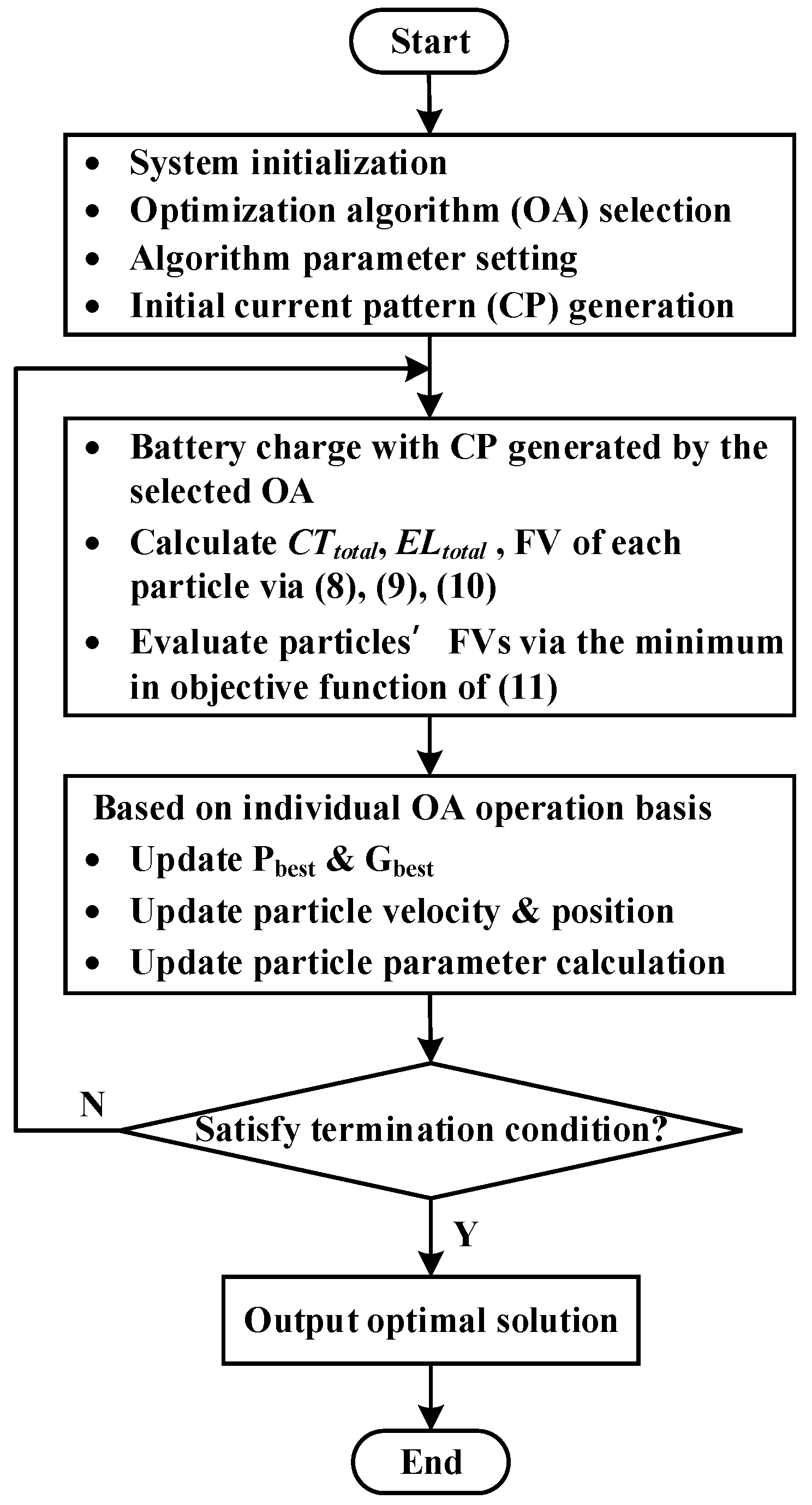
Figure 10 shows the general operation flowchart of the MSCC charging method based on the OA. No matter which OA is adopted, this process can generally be used to search for the OCCP. The search steps for the OCCP are explained as follows:
- Step (1)
- First, execute system and particle parameter initialization and select OA to be applied. Then, perform parameter setting for the selected OA, and the initial charging current pattern is generated. In this study, according to the theoretical analysis of the problem described in Section 2.2, each particle can be set as a five-dimensional vector composed of [Vcut-off, I1, I2, I3, I4]. Where the transition voltage Vcut-off and the current I1~I4 are the five variables that need to be determined and optimized for each particle.
- Step (2)
- The battery is charged with the current pattern generated by the selected OA. From the charging data recorded, calculate the total CT, total EL, and FV of each particle via (8)–(10), respectively, and then evaluate and rank the FV of each particle according to the value obtained from the objective function of (11). The particle position with the minimal FV is regarded as the current best solution.
- Step (3)
- Based on the FV of each particle obtained from Step (2), update the individual best Pbest and the group best Gbest with the separate operation principles of different OAs and then update the velocity and position of each particle. Finally, the dominant parameters involved in the OA for manipulating the searching process of each particle should also be recalculated and updated for correct utilization in the next iteration.
- Step (4)
- Check whether the convergence criteria are satisfied or not. If not, return to Step (2) to continue execution. If the convergence conditions are met, output the OCCP and end the searching process.
Figure 10.
Operation flowchart of the BIOA-based MSCC charging strategy.

4. Experimental Results and Discussion
4.1. Computation Parameter Setting and Results
Table 1 lists the parameters required for the calculation of the CTtotal, ELtotal, and FV. The OCVs at SOC 100% and 0% are measured at an ambient temperature of 25 °C, and the proportional weight σ in the objective function is set to 0.5, which means that CT and EL have equivalent significance. As mentioned in Section 2.2, the factors affecting CT and EL include each stage current (I1~I5) and the cut-off voltage (Vcut-off) for current transition. Generally, the I1~I5 is set between 0 C and 1 C, and the Vcut-off is set to 4.2 V. The range setting of variables in the particle is tabulated in Table 2. It should be noted that to prevent the battery from damage, these parameter values must ensure that the OCV does not exceed the rated voltage during the entire charging process. Table 3 shows the main parameter setting of the BIOAs used in this paper. The computation is run on a personal computer (PC) with a CPU of i7-13700 16C24T.
To verify the correctness and feasibility of the proposed charging methods, the simulations under various test scenarios are performed. Generally, most BIOAs involve random parameters to enable them to escape the local optima. Due to the random variation in these parameters, the best solution found after each execution tends to be different. Therefore, in order to obtain effective optimal solutions, the average value of the OCCP for each BIOA case is executed 50 times under the setting of 100 iterations, and the number of particles of 50, 100, 200, and 300, respectively, is taken as the final OCCP. In this study, apart from the proposed five BIOA-based methods, three additional cases, as well as the FC method proposed in [36] and the conventional CC-CV method, are also run to demonstrate that the OCCP obtained has the optimal solution. Table 4 shows the simulation results in terms of four CPEIs, including the best FV (FVbest), CTtotal, ELtotal, and CHC. The obtained OCCP corresponding to each simulation case listed in Table 4 is tabulated in Table 5. From Table 4, the FC method has the best CT performance because this research aims to minimize the CT, i.e., it is a special case in (11) for setting σ = 1. In addition, the CC-CV method usually has better performance in CHC. However, if the objective function must satisfy both the performance of CT and EL, it can be seen from the FVbest indicator that the proposed methods have a significant improvement in FVbest than that obtained by using the FC and CC-CV methods. Among them, case-JSA has the best simulation FV, and it shows 54.1% and 65.6% improvement in FV compared with CC-CV and FC methods, respectively. On the other hand, additional three cases, including PSO − 0.1 A, GWO + 0.1 A, and JSA + 0.1 A, formed by fine-tuning the values of I1~I4 in the optimal case-PSO, -GWO, and -JSA by subtracting 0.1 A and adding 0.1 A, are conducted to further confirm the correctness of the obtained OCCP. Similarly, it is obvious from the FVbest indicator that even a solution that is very close to the optimal solution does not have the best FV.
4.2. Experimental Test Environment Setup and Results
As described in the previous subsection, the proposed BIOA-based algorithms are executed on a MATLAB-based computation platform to obtain the OCCP. Subsequently, it is necessary to conduct actual battery charge and discharge, record relevant data, and calculate the corresponding CPEI to verify that the OCCP obtained is indeed optimal. In this study, the CT4008T battery charge–discharge tester from BioLogic is used to perform battery charge–discharge experiments and data measurement. During the experiment, the battery is placed in the DDTH-48L-00-BP4.3 thermostatic chamber, and the temperature is controlled at 25 °C. Figure 11 shows the experimental platform architecture set up in this study. The experimental procedure first inputs and sets the required charging current values deriving from the current patterns listed in Table 5, then charges and records the charging data and CPEIs (CT, CHC, TR). After resting for 3 h, discharge the battery with 0.2 C CC until the OCV reaches 3 V, then record the discharge data and DHC, and calculate CE. If all charging current patterns have been run, the operating procedure is terminated. The experimental results in terms of eight CPEIs, including CT, CHC, discharging capacity (DHC), CE, CWh, discharging energy (DWh), ATR, and FV, are illustrated in Table 6. It is worth noting that the experimental results shown in Table 6 are obtained by specifying the charging current values of each case the same as those in the OCCP derived from the computation of the optimization algorithms. From Table 6, it can be seen that, in all the test scenarios, the capacity charged by using the proposed methods is more than 99% of the CC-CV method under the lowest ATR and the highest CE. Furthermore, the experimental results are in good agreement with those obtained from the computation.
On the other hand, to further highlight the effectiveness and performance improvement in this study, the conventional CC-CV and FC methods are employed as the primary benchmark for the comparison with the proposed MSCC charging methods. For a fair comparison, the CC-phase current is set to 1.6 A (0.49 C), which is equivalent to the average value of all the first-stage currents obtained by using the proposed methods, and the charging cut-off current is set to 0.02 C. Comparing with the CC-CV and FC methods, the IRs of the proposed methods in individual CPEI are shown in Table 7 and Table 8, respectively. From Table 7, the maximum IRs in terms of the CT, CHC, CE, CWh, ATR, and FV are 21.10%, 0.40%, 0.24%, 2.85%, 18.86%, and 68.99%, respectively, which are contributed, respectively, by case-MPSO, case-JSA, case-GWO, case-MPSO, case-MGWO, and case-MPSO. Similarly, the maximum IRs in terms of the CHC, CE, CWh, ATR, and FV, from the comparison with the FC method in Table 8, are 0.39%, 0.53%, 3.52%, 29.35%, and 47.72%, respectively, which are contributed, respectively, by case-JSA, case-GWO, case-MPSO, case-MGWO, and case-MPSO. It should be noted that, in Table 6, the FC method has the shortest CT. The reason is that the FC method focuses on CT minimization, which is equivalent to a special case of setting the proportional weight of the objective function to one, so the IRs in this indicator are all negative.
In addition, it is difficult to directly measure the energy loss when conducting battery charging experiments, but the energy loss is directly related to the TR observed. Therefore, in this work, the charging TR is used as an evaluation indicator for EL performance during the test. Figure 12 shows the measured curves of charging TR for various charging methods. From Figure 12, it can be seen that the FC and CC-CV methods exhibit significant variations in accumulated TR, especially the FC method. This is because the charging loss indicator is not taken into account, leading to a substantial increase in TR. On the other hand, the proposed methods show similar TR curves with smoother variations because the balance between CT and EL is considered. Compared with the FC and CC-CV methods, the proposed method achieves maximum IRs in ATR of 29.35% and 18.86%, respectively, both contributed by case-MGWO. Figure 13, Figure 14, Figure 15, Figure 16 and Figure 17 show the simulated and experimental waveforms, including battery current, voltage, and capacity, measured under the charge of OCCP found by using the proposed methods. Figure 18 and Figure 19 illustrate the simulated and experimental waveforms deriving from the charge of the FC and CC-CV methods. It is obvious from these measured waveforms that the experimental and simulation results match significantly. It verifies that the built battery ECM, developed computation platform, and the constructed experimental environment are correct and valid. It also proves that the experimental results are in good agreement with the theoretical derivation.
4.3. Comprehensive Evaluation of the Proposed BIOA-Based Algorithms
This study extensively evaluates five BIOA-based charging methods based on five CPEIs, including CT, CHC, CE, CWh, and ATR. The evaluation results can serve as a recommendation reference for the suitable charging method for LiBs with different charging performance requirements in various application scenarios. The radar chart analysis is utilized to perform the comprehensive evaluation. According to the experimental results shown in Table 6, the obtained radar chart is shown in Figure 20, and the corresponding evaluation scores are listed in Table 9. The scoring rule for each performance indicator is divided into two types: “the higher, the better” or “the lower, the better”. For example, the smaller the CT value, the higher the score, while the larger the CE value, the higher the score, and so on.
It can be seen from Table 9 that MPSO has the best performances in CWh and ATR indicators, MGWO has the best ATR performance, GWO is good at obtaining high CE and CWh, the JSA has the best CHC and ATR performances, and the FC is dedicated to improving the CT performance, while the performances for the rest of the methods are average. According to the ranking of the total scores of various performance indicators, the top three with the best overall performance are the methods of JSA, MPSO, and GWO. That is, from the comprehensive evaluation results of the radar chart, the suggestion of charging method adoption can be made as follows: for the most energy-saving charging, MPSO and GWO can be chosen. MPSO, MGWO, and JSA are good for controlling the TR during charge. If the goal is to charge the battery with the maximum capacity, the JSA is a good choice. Additionally, GWO can also be used to obtain high charging efficiency. The FC method can effectively reduce charging time.
5. Conclusions
To reduce the numerous time-consuming charge-and-discharge experiments and take the capability of wide-range search in the solution space into account, in this paper, the OCCP of the MSCC is solved by using the proposed five BIOA-based methods, including PSO, MPSO, GWO, MGWO, and the JSA, which is run on the MATLAB-based computation platform constructed to minimize the objective function of combining CT and EL with a proportional weight. Without the need for a substantial and tedious experimental process, the OCCP search can be rapidly achieved only through the battery ECM developed on the computation platform. The theoretical derivation and validity were confirmed through the simulation and experimental results, which demonstrate that the OCCPs obtained by all the devised charging strategies possess the lowest fitness values and the best charging performance as compared with their counterparts. Among them, the fitness value acquired by MPSO outperforms those of all the other charging methods studied.
The experimental results show that the maximum IRs of the studied techniques in six CPEIs of CT, CHC, CE, CWh, ATR, and FV, are 21.10%, 0.40%, 0.24%, 2.85%, 18.86%, and 68.99% which are contributed, respectively, by MPSO, JSA, GWO, MPSO, MGWO, and MPSO, as compared with the traditional CC-CV method. Similarly, the maximum IRs in terms of five performance indicators, CHC, CE, CWh, ATR, and FV, from the comparison with the FC method, are 0.39%, 0.53%, 3.52%, 29.35%, and 47.72%, respectively, which are contributed, respectively, by the JSA, GWO, MPSO, MGWO, and MPSO. In addition, compared with the FC and CC-CV methods, the proposed method achieves maximum IRs in ATR of 29.35% and 18.86%, respectively, both contributed by MGWO. On the other hand, a comprehensive evaluation of the proposed BIOA-based algorithms via the radar chart analysis was conducted to make recommendations for charging method adoption. The recommendations of charging methods adopted can be made as follows: the MPSO and GWO methods can be chosen to perform the most energy-saving charge. MPSO, MGWO, and the JSA are good at controlling the TR during charge. The JSA method has the ability of maximum-capacity charge. In addition, GWO can be adopted to obtain the best charging efficiency, and the FC method can charge the battery with a significant reduction in charging time.
Author Contributions
Conceptualization, S.-C.W.; methodology, S.-C.W.; software, Z.-Y.Z.; validation, S.-C.W. and Z.-Y.Z.; writing—original draft preparation, S.-C.W.; writing—review and editing, S.-C.W. All authors have read and agreed to the published version of the manuscript.
Funding
This research was funded by the National Science and Technology Council (NSTC), Taiwan, grant number MOST 111-2221-E-019-026-MY2.
Data Availability Statement
Data are contained within the article.
Acknowledgments
The authors would like to thank the National Science and Technology Council of Taiwan for the project grant to complete this research.
Conflicts of Interest
The authors declare no conflict of interest.
References
- Pohlmann, S.; Mashayekh, A.; Kuder, M.; Neve, A.; Weyh, T. Data Augmentation and Feature Selection for the Prediction of the State of Charge of Lithium-Ion Batteries Using Artificial Neural Networks. Energies 2023, 16, 6750. [Google Scholar] [CrossRef]
- Pelosi, D.; Longo, M.; Zaninelli, D.; Barelli, L. Experimental Investigation of Fast−Charging Effect on Aging of Electric Vehicle Li−Ion Batteries. Energies 2023, 16, 6673. [Google Scholar] [CrossRef]
- Bilansky, J.; Lacko, M.; Pastor, M.; Marcinek, A.; Durovsky, F. Improved Digital Twin of Li-Ion Battery Based on Generic MATLAB Model. Energies 2023, 16, 1194. [Google Scholar] [CrossRef]
- Zhang, R.; Li, X.; Sun, C.; Yang, S.; Tian, Y.; Tian, J. State of Charge and Temperature Joint Estimation Based on Ultrasonic Reflection Waves for Lithium-Ion Battery Applications. Batteries 2023, 9, 335. [Google Scholar] [CrossRef]
- Xu, J.; Sun, C.; Ni, Y.; Lyu, C.; Wu, C.; Zhang, H.; Yang, Q.; Feng, F. Fast Identification of Micro-Health Parameters for Retired Batteries Based on a Simplified P2D Model by Using Padé Approximation. Batteries 2023, 9, 64. [Google Scholar] [CrossRef]
- Song, D.; Wang, S.; Di, L.; Zhang, W.; Wang, Q.; Wang, J.V. Lithium-Ion Battery Life Prediction Method under Thermal Gradient Conditions. Energies 2023, 16, 767. [Google Scholar] [CrossRef]
- Gemma, F.; Tresca, G.; Formentini, A.; Zanchetta, P. Balanced Charging Algorithm for CHB in an EV Powertrain. Energies 2023, 16, 5565. [Google Scholar] [CrossRef]
- Kwak, B.; Kim, M.; Kim, J. Add-On Type Pulse Charger for Quick Charging Li-Ion Batteries. Electronics 2020, 9, 227. [Google Scholar] [CrossRef]
- Tsang, K.M.; Chan, W.L. Current Sensorless Quick Charger for Lithium-ion Batteries. Energy Convers. Manag. 2011, 52, 1593–1595. [Google Scholar] [CrossRef]
- Notten, P.H.L.; Op het Veld, J.H.G.; van Beek, J.R.G. Boostcharging Li-ion Batteries: A Challenging New Charging Concept. J. Power Source 2005, 145, 89–94. [Google Scholar] [CrossRef]
- Chen, L.R.; Hsu, R.C.; Liu, C.S. A Design of a Grey-Predicted Li-Ion Battery Charge System. IEEE Trans. Ind. Electron. 2008, 55, 3692–3701. [Google Scholar] [CrossRef]
- Hsieh, G.C.; Chen, L.R.; Huang, K.S. Fuzzy Controlled Lithium-ion Battery Charge System with Active State of Charge Controller. IEEE Trans. Ind. Electron. 2001, 48, 585–593. [Google Scholar] [CrossRef]
- Chen, L.R.; Chen, J.J.; Chu, N.Y.; Han, G.Y. Current pumped battery charger. IEEE Trans. Ind. Electron. 2008, 55, 2482–2488. [Google Scholar] [CrossRef]
- Patnaik, L.; Praneeth, A.V.J.S.; Williamson, S.S. A Closed-Loop Constant-Temperature Constant-Voltage Charging Technique to Reduce Charge Time of Lithium-Ion Batteries. IEEE Trans. Ind. Electron. 2019, 66, 1059–1067. [Google Scholar] [CrossRef]
- Fang, H.; Depcik, C.; Lvovich, V. Optimal Pulse-modulated Lithium-ion Battery Charging Algorithms. J. Energy Storage 2018, 15, 359–367. [Google Scholar] [CrossRef]
- Wang, S.C.; Chen, G.J.; Liu, Y.H. Adaptive Charging Strategy with Temperature Rise Mitigation and Cycle Life Extension for Li-ion Batteries. CPSS Trans. Power Electron. Appl. 2018, 3, 202–212. [Google Scholar] [CrossRef]
- Gao, Y.; Zhang, X.; Guo, B.; Zhu, C.; Wiedemann, J.; Wang, L.; Cao, J. Health-aware Multiobjective Optimal Charging Strategy with Coupled Electrochemical-thermal-aging Model for Lithium-ion Battery. IEEE Trans. Ind. Inform. 2020, 16, 3417–3429. [Google Scholar] [CrossRef]
- Bohinsky, A.; Rangarajan, S.P.; Barsukov, Y.; Mukherjee, P.P. Preventing Lithium Plating during Fast Charging of Lithium Ion Cells. ECS Meet. Abstr. 2020, MA2020-02, 594. [Google Scholar] [CrossRef]
- Chen, L.R. A Design of an Optimal Battery Pulse Charge System by Frequency-Varied Technique. IEEE Trans. Ind. Electron. 2007, 54, 398–405. [Google Scholar] [CrossRef]
- Chen, L.R. Design of Duty-Varied Voltage Pulse Charger for Improving Li-Ion Battery-Charging Response. IEEE Trans. Ind. Electron. 2009, 56, 480–487. [Google Scholar] [CrossRef]
- Purushothama, B.K.; Morrison, P.W., Jr.; Landau, U. Reducing Mass-Transport Limitations by Application of Special Pulsed Current Modes. J. Electrochem. Soc. 2005, 152, 33–39. [Google Scholar] [CrossRef]
- Purushothama, B.K.; Landau, U. Rapid Charging of Lithium-ion Batteries Using Pulsed Currents. J. Electrochem. Soc. 2006, 153, 533–542. [Google Scholar] [CrossRef]
- Isuru Niroshana, S.M.; Sirisukprasert, S. Adaptive Pulse Charger for Li-ion Batteries. In Proceedings of the 8th International Conference of Information and Communication Technology for Embedded Systems (IC-ICTES), Chonburi, Thailand, 7–9 May 2017. [Google Scholar]
- Liu, Y.H.; Teng, J.H.; Lin, Y.C. Search for an Optimal Rapid Charging Pattern for Li-ion Batteries Using Ant Colony System Algorithm. IEEE Trans. Ind. Electron. 2005, 52, 1328–1336. [Google Scholar] [CrossRef]
- Liu, Y.H.; Luo, Y.F. Search for an Optimal Rapid Charging Pattern for Li-ion Batteries Using Taguchi Approach. IEEE Trans. Ind. Electron. 2010, 57, 3963–3971. [Google Scholar] [CrossRef]
- Liu, Y.H.; Hsieh, C.H.; Luo, Y.F. Search for an Optimal Rapid Charging Pattern for Li-ion Batteries Using Consecutive Orthogonal Arrays. IEEE Trans. Ind. Electron. 2011, 26, 654–661. [Google Scholar]
- Dung, L.R.; Yen, J.H. ILP-based Algorithm for Lithium-ion Battery Charging Profile. In Proceedings of the 2010 IEEE International Symposium on Industrial Electronics, Bari, Italy, 4–7 July 2010; pp. 2286–2291. [Google Scholar]
- Attia, P.M.; Grover, A.; Jin, N.; Severson, K.A.; Markov, T.M.; Liao, Y.H.; Chen, M.H.; Cheong, B.; Perkins, N.; Yang, Z.; et al. Closed-loop Optimization of Fast-Charging Protocols for Batteries with Machine Learning. Nature 2020, 578, 397–402. [Google Scholar] [CrossRef]
- Vo, T.T.; Chen, X.; Shen, W.; Kapoor, A. New Charging Strategy for Lithium-ion Batteries based on the Integration of Taguchi Method and State of Charge Estimation. J. Power Sources 2015, 273, 413–422. [Google Scholar] [CrossRef]
- Lee, C.H.; Chen, M.Y.; Hsu, S.H.; Jiang, J.A. Implementation of a SOC-based Four-stage Constant Current Charger for Li-ion Batteries. J. Energy Storage 2018, 18, 528–537. [Google Scholar] [CrossRef]
- Lee, C.H.; Chang, T.W.; Hsu, S.H.; Jiang, J.A. Taguchi-based PSO for Searching an Optimal Four-stage Charge Pattern of Li-ion Batteries. J. Energy Storage 2019, 21, 301–309. [Google Scholar] [CrossRef]
- Jiang, L.; Huang, Y.D.; Li, Y.; Yu, J.Q.; Qiao, X.B.; Huang, C.; Cao, Y.J. Optimization of Variable-Current Charging Strategy Based on SOC Segmentation for Li-Ion Battery. IEEE Trans. Intell. Transp. Syst. 2021, 22, 622–629. [Google Scholar] [CrossRef]
- Wang, S.C.; Liu, Y.H. A PSO-Based Fuzzy-Controlled Searching for the Optimal Charge Pattern of Li-Ion Batteries. IEEE Trans. Ind. Electron. 2015, 62, 2983–2993. [Google Scholar] [CrossRef]
- Makeen, P.; Ghali, H.A.; Memon, S. Experimental and Theoretical Analysis of the Fast Charging Polymer Lithium-Ion Battery Based on Cuckoo Optimization Algorithm (COA). IEEE Access 2020, 8, 140486–140496. [Google Scholar] [CrossRef]
- Chen, G.J.; Liu, Y.H.; Wang, S.C.; Luo, Y.F.; Yang, Z.Z. Searching for the Optimal Current Pattern Based on Grey Wolf Optimizer and Equivalent Circuit Model of Li-ion Batteries. J. Energy Storage 2021, 33, 101933. [Google Scholar] [CrossRef]
- Khan, A.B.; Choi, W. Optimal Charge Pattern for the High-Performance Multistage Constant Current Charge Method for the Li-ion Batteries. IEEE Trans. Energy Convers. 2018, 33, 1132–1140. [Google Scholar] [CrossRef]
- Eberhart, R.C.; Shi, Y.H. Particle Swarm Optimization: Developments, Applications and Resources. In Proceedings of the 2001 Congress on Evolutionary Computation (IEEE Cat. No. 01TH8546), Seoul, Republic of Korea, 27–30 May 2001; pp. 81–86. [Google Scholar]
- Mirjalili, S.; Mirjalili, S.M.; Lewis, A. Grey Wolf Optimizer. Adv. Eng. Softw. 2014, 69, 46–61. [Google Scholar] [CrossRef]
- Chou, J.S.; Truong, D.N. A Novel Metaheuristic Optimizer Inspired by Behavior of Jellyfish in Ocean. Appl. Math. Comput. 2021, 389, 125535. [Google Scholar] [CrossRef]
Figure 4.
Schematic waveforms of MSCC method.

Figure 5.
Schematic diagram of fitness-value function derivation.

Figure 6.
Particle velocity and position update concept in PSO searching.

Figure 7.
Mechanism of the gray wolf position update.

Figure 8.
Curves of under different ρ values.

Figure 11.
The experimental platform architecture.

Figure 12.
Measured curves of TR for various charging methods.

Figure 13.
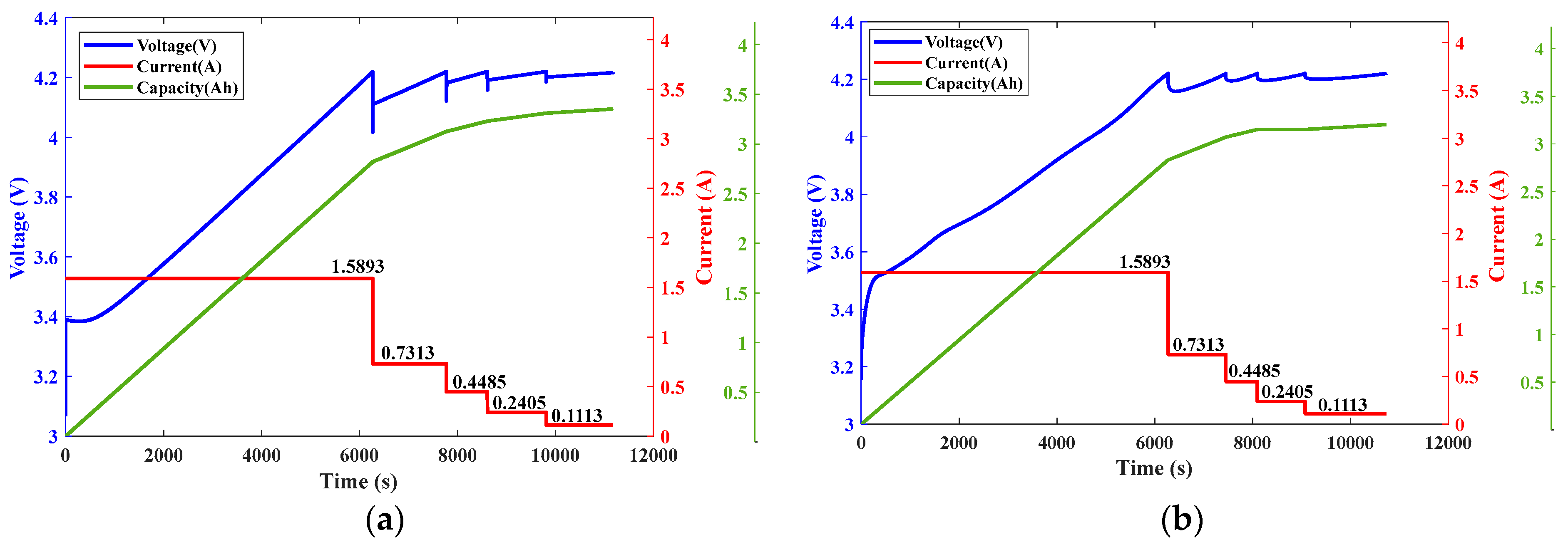
Charging waveforms of MPSO method: (a) simulation; (b) experiment.

Figure 14.
Charging waveforms of PSO method: (a) simulation; (b) experiment.

Figure 15.
Charging waveforms of MGWO method: (a) simulation; (b) experiment.

Figure 16.
Charging waveforms of GWO method: (a) simulation; (b) experiment.

Figure 17.
Charging waveforms of JSA method: (a) simulation; (b) experiment.

Figure 18.
Charging waveforms of FC method: (a) simulation; (b) experiment.

Figure 19.
Charging waveforms of CC-CV method: (a) simulation; (b) experiment.

Figure 20.
Radar chart of comprehensive performance evaluation.


Table 1.
Parameters for CTtotal, ELtotal, and FV computation.
| For CTtotal and ELtotal Calculation | For FV Calculation | ||
|---|---|---|---|
| Rated capacity | 3.3 Ah | CTmax | 14,496 s |
| VCeq at 100% SOC | 4.2 V | CTmin | 9894 s |
| VCeq at 0% SOC | 3.0662 V | ELmax | 5298.3 J |
| Req | As Equation (1) | ELmax | 1926.8 J |
| Ceq | 10,478 F | σ | 0.5 |
Table 2.
Range setting of variables in the particle.
| Vcut-off (V) | I1 (A) | I2 (A) | I3 (A) | I4 (A) | I5 (A) |
|---|---|---|---|---|---|
| 4.2~4.22 | 0~3.3 | 0~3.3 | 0~3.3 | 0~3.3 |
Table 3.
Parameter setting of the used BIOAs.
| Algorithm | Iteration No. | Particle No. | Main Parameters |
|---|---|---|---|
| MPSO | 100 | 200 | c1 = 1, c2 = 2, ω, c3 = 2~0 |
| PSO | 100 | 200 | c1 = 1, c2 = 2, ω = 2~0 |
| MGWO | 100 | 200 | ρ = 30 |
| GWO | 100 | 200 | N/A |
| JSA | 100 | 200 | β = 3, γ = 0.1 |
Table 4.
Simulation results.
| Case | FVbest | CTtotal (s) | ELtotal (J) | CHC (Ah) |
|---|---|---|---|---|
| MPSO | 0.2687 | 10,328 | 2960.03 | 3.2950 |
| PSO | 0.2796 | 11,058 | 2953.17 | 3.2977 |
| MGWO | 0.2809 | 11,046 | 2926.93 | 3.2924 |
| GWO | 0.2810 | 10,780 | 2930.12 | 3.2913 |
| JSA | 0.2700 | 11,400 | 2872.64 | 3.2882 |
| PSO − 0.1 A | 0.3618 | 11,814 | 2727.87 | 3.2920 |
| GWO + 0.1A | 0.3053 | 10,885 | 3088.43 | 3.2907 |
| JSA + 0.1 A | 0.3977 | 11,829 | 3033.13 | 3.3021 |
| FC [36] | 0.7857 | 9216 | 5559.78 | 3.2908 |
| 0.7 C CC-CV | 0.3458 | 11,449 | 3118.50 | 3.2936 |
Table 5.
Obtained OCCP of each simulation case in line with Table 4.
Table 5.
Obtained OCCP of each simulation case in line with Table 4.
| Case | Vcut_off (V) | I1 (A) | I2 (A) | I3 (A) | I4 (A) | I5 (A) |
|---|---|---|---|---|---|---|
| MPSO | 4.22 | 1.6348 | 0.9003 | 0.3640 | 0.2308 | 0.1578 |
| PSO | 4.22 | 1.6185 | 0.8255 | 0.4453 | 0.2405 | 0.1345 |
| MGWO | 4.22 | 1.6153 | 0.8028 | 0.4355 | 0.2438 | 0.1250 |
| GWO | 4.22 | 1.6153 | 0.8515 | 0.4485 | 0.2373 | 0.1337 |
| JSA | 4.22 | 1.5893 | 0.7313 | 0.4485 | 0.2405 | 0.1113 |
| PSO − 0.1 A | 4.22 | 1.5185 | 0.7255 | 0.3453 | 0.1405 | 0.1345 |
| GWO + 0.1 A | 4.22 | 1.7153 | 0.9515 | 0.5485 | 0.3373 | 0.1337 |
| JS + 0.1 A | 4.22 | 1.6893 | 0.8313 | 0.5485 | 0.3405 | 0.1113 |
| FC [36] | 4.22 | 3.3 | 1.3539 | 0.5554 | 0.2278 | 0.0935 |
| 0.7 C CC-CV | 4.2 | 2.31 | − | − | − | − |
Table 6.
Summary of experimental results.
| Case | CT (s) | CHC (Ah) | DHC (Ah) | CE (%) | CWh (Wh) | DWh (Wh) | ATR (°C) | FV |
|---|---|---|---|---|---|---|---|---|
| MPSO | 9694 | 3.1913 | 3.1713 | 99.37 | 12.16 | 11.0993 | 2.09 | 0.1414 |
| PSO | 9994 | 3.1993 | 3.1763 | 99.28 | 12.40 | 11.3497 | 2.46 | 0.2208 |
| MGWO | 10,374 | 3.1932 | 3.1719 | 99.33 | 12.23 | 11.1666 | 2.08 | 0.2117 |
| GWO | 9974 | 3.1962 | 3.1773 | 99.41 | 12.38 | 11.3528 | 2.53 | 0.2303 |
| JSA | 10,729 | 3.2076 | 3.1828 | 99.23 | 12.42 | 11.3748 | 2.30 | 0.2687 |
| FC [36] | 9150 | 3.1952 | 3.1597 | 98.89 | 12.60 | 11.2753 | 2.94 | 0.2705 |
| 0.49 C CC-CV | 12,286 | 3.1949 | 3.1684 | 99.17 | 12.52 | 11.3454 | 2.56 | 0.4560 |
Table 7.
IRs of proposed methods compared with CC-CV method.
| Case | CT (s) | CHC (Ah) | CE (%) | CWh (Wh) | ATR (°C) | FV |
|---|---|---|---|---|---|---|
| MPSO | 21.10% | 0.11% | 0.20% | 2.85% | 18.36% | 68.99% |
| PSO | 18.66% | 0.14% | 0.11% | 0.92% | 7.72% | 54.96% |
| MGWO | 15.56% | 0.05% | 0.16% | 2.32% | 18.86% | 53.57% |
| GWO | 18.82% | 0.04% | 0.24% | 1.12% | 1.17% | 49.51% |
| JSA | 12.67% | 0.40% | 0.06% | 0.76% | 10.20% | 41.08% |
Table 8.
IRs of proposed methods compared with FC method.
| Case | CT (s) | CHC (Ah) | CE (%) | CWh (Wh) | ATR (°C) | FV |
|---|---|---|---|---|---|---|
| MPSO | −5.95% | 0.12% | 0.49% | 3.52% | 28.91% | 47.72% |
| PSO | −9.22% | 0.13% | 0.39% | 1.61% | 16.24% | 24.07% |
| MGWO | −13.38% | 0.06% | 0.44% | 2.99% | 29.35% | 21.73% |
| GWO | −9.01% | 0.03% | 0.53% | 1.81% | 13.95% | 14.88% |
| JSA | −17.26% | 0.39% | 0.34% | 1.44% | 21.80% | 0.67% |
Table 9.
Score corresponding to the radar chart.
| CASE | CT (s) | CHC (Ah) | CE (%) | CWh (Wh) | ATR (°C) | Total Score |
|---|---|---|---|---|---|---|
| MPSO | 0.8265 | 0.0000 | 0.9231 | 1.0000 | 1.0000 | 3.7496 |
| PSO | 0.7309 | 0.3465 | 0.7500 | 0.8898 | 0.7450 | 3.4621 |
| MGWO | 0.6097 | 0.1166 | 0.8462 | 0.8501 | 1.0000 | 3.4225 |
| GWO | 0.7372 | 0.1024 | 1.0000 | 1.0000 | 0.6396 | 3.4792 |
| JSA | 0.4965 | 1.0000 | 0.6538 | 0.7989 | 1.0000 | 3.9493 |
| FC [36] | 1.0000 | 0.0236 | 0.0000 | 0.0000 | 0.0000 | 1.0236 |
| 0.49 C CC-CV | 0.0000 | 0.0000 | 0.5385 | 0.3819 | 0.5928 | 1.5131 |
Disclaimer/Publisher’s Note: The statements, opinions and data contained in all publications are solely those of the individual author(s) and contributor(s) and not of MDPI and/or the editor(s). MDPI and/or the editor(s) disclaim responsibility for any injury to people or property resulting from any ideas, methods, instructions or products referred to in the content. |
© 2023 by the authors. Licensee MDPI, Basel, Switzerland. This article is an open access article distributed under the terms and conditions of the Creative Commons Attribution (CC BY) license (https://creativecommons.org/licenses/by/4.0/).
Share and Cite
MDPI and ACS Style
Wang, S.-C.; Zhang, Z.-Y. Research on Optimum Charging Current Profile with Multi-Stage Constant Current Based on Bio-Inspired Optimization Algorithms for Lithium-Ion Batteries. Energies 2023, 16, 7641. https://doi.org/10.3390/en16227641
AMA Style
Wang S-C, Zhang Z-Y. Research on Optimum Charging Current Profile with Multi-Stage Constant Current Based on Bio-Inspired Optimization Algorithms for Lithium-Ion Batteries. Energies. 2023; 16(22):7641. https://doi.org/10.3390/en16227641
Chicago/Turabian StyleWang, Shun-Chung, and Zhi-Yao Zhang. 2023. "Research on Optimum Charging Current Profile with Multi-Stage Constant Current Based on Bio-Inspired Optimization Algorithms for Lithium-Ion Batteries" Energies 16, no. 22: 7641. https://doi.org/10.3390/en16227641
Note that from the first issue of 2016, this journal uses article numbers instead of page numbers. See further details here.