
On the Thermal Stability of a Counter-Current Fixed-Bed Gasifier

Institute of Energy Process Engineering and Fuel Technology, Clausthal University of Technology, Agricolastrasse 4, 38678 Clausthal-Zellerfeld, Germany
*
Author to whom correspondence should be addressed.
Energies 2023, 16(9), 3762; https://doi.org/10.3390/en16093762
Submission received: 6 March 2023
/
Revised: 18 April 2023
/
Accepted: 20 April 2023
/
Published: 27 April 2023
(This article belongs to the Special Issue Pyrolysis and Gasification of Biomass and Waste II)
Abstract
:In recent years, gasification gained attention again, both as an industrial application and as a research topic. This trend has led to the necessity to understand the process and optimize reactors for various materials and configurations. In this article, the thermal structure of a counter-current reactor is investigated to demonstrate that constraints on the temperature mainly determine the oxidation and the pyrolysis region. A non-dimensional set of equations is written and numerically solved using the method of lines (MOL) with spatial discretization based on a spectral algorithm. The results show that four thermal structures can be identified, two of which are the most common ones found in reactors of practical applications. Two stationary operation positions have been determined, one in the upper and one in the lower part of the reactor. Existence and stability conditions have been discussed based on non-dimensional parameters. The knowledge derived from this analysis was applied to two configurations, one typical of a biomass gasifier and one proposed for waste gasification.
1. Introduction
Gasification is a well-known technology that has been used in industrial plants for nearly 200 years. In the beginning, coal and peat were used to produce light gases for energy or heat production. In fact, conversion of heterogeneous materials into light gaseous fuels such as methane, carbon monoxide, and hydrogen made it possible to increase the efficiency because of the higher adiabatic temperature. Later on, other technologies replaced gasification in the energy sector, and only recently, gasification gained attention again, both as an industrial application and as a research topic. In particular, gasification of less calorific fuels (peat, biomass, plastics, and various kind of wastes) has become of considerable importance in the current energy scenario due to both resources protection and climate precaution, specifically CO2 neutrality (see for the example [1,2,3,4,5,6,7]). Nevertheless, the recycling aspects of the thermal treatment of complex materials for the modern circular economy [8,9,10] are no less important.
The change of feedstock materials requires, in addition to the knowledge of chemical reactions, their products, and their dependence on thermodynamic variables, a thorough and accurate knowledge of the functioning of the reactors used in the various processes. This article proposes an original approach to the mathematical analysis of a particular type of reactor, namely the counter-current (updraft) reactor.
Several types of reactors are currently available for biomass gasification: counter-current fixed bed, co-current fixed bed, fluidized bed, entrained flow, plasma, and free radical reactors. Studies conducted by Gomez-Barea and Leckner [11] reviewed the fluidized-bed technology, Higman [12] studied the entrained-flow gasifiers, while Chopra et al. [13,14] studied the fixed-bed technology. In the present day, there has been a resurgence of interest in this technology, as evidenced by the numerous publications available in the literature. In entrained flow gasifiers, a dry pulverized solid, an atomized liquid fuel, or a fuel slurry is gasified with an enriched oxygen agent in co-current flow. High temperatures and pressures cause a high throughput; however, thermal efficiency is somewhat low, as the gas must be cooled before it can be cleaned with existing technology [15,16]. The fuel is fluidized in oxygen and steam or air in fluidized-bed reactors. Since temperatures are usually relatively low, the fuel must be highly reactive. Fuel throughput is higher than in the fixed bed technology but not as high as in the entrained flow gasifier [11,17,18,19,20,21]. In co-current fixed-bed gasifiers (also known as downdraft type), the gasification agent flows in the same direction as the fuel (downwards, hence the name). Heat needs to be added to the upper part of the reactor, either by oxidizing a small amount of fuel or from external heat sources. The produced gas leaves the gasifier at a high temperature, but since most of this heat can be often transferred to the gasification agent injected at the top of the bed, the resulting energy efficiency is similar to the one achievable with the counter-current reactor type. Since the gas must pass through the hot bed, the tar level is much lower than in the counter-current reactors [13,22,23,24,25,26,27,28]. In counter-current fixed-bed gasifiers (also known as updraft type), the gasification agent and the solid fuel flow in a counter-current configuration. The throughput for this type of reactor is relatively low, while the thermal efficiency is high as the temperatures in the gas exit are relatively low. However, as a consequence, tar and methane production is significant in typical operation conditions, so the product gas must be extensively cleaned before use [29,30,31,32,33,34,35,36].
Despite their advantages and decades of economic and scientific efforts, the fixed-bed gasification process, especially on industrial scales, has yet to establish itself in the market. The low efficiency of the co-current process, the high tar content in the gas in the counter-current process, and the resulting high costs for gas and wastewater treatment often lead to the limits of economic viability. For example, the most recent developments in Germany are based on the entrained-flow technology instead and include the Bioliq reactor [5,15], and TU Freiberg entrained-flow gasifier [37]. In combination with these intense research activities, efforts have also been made, in the recent past, to develop processes for clean thermal treatment of the most challenging fuels, such as biomass, substitute fuels (RDF), and waste with high proportions of chlorine, sulfur, but also heavy metals. In particular, among the various projects started recently, the Ecoloop process [38,39,40] was an attempt at a new innovative counter-flow gasifier that converts various carbonaceous materials into purified syngas. The Ecoloop process was based on a counter-current moving-bed gasifier with a high proportion of calcined mineral rock. This material, almost chemically inert, serves as a support structure and allows the primary cracking of tars, and, simultaneously, is responsible for binding halogens, sulfur, and heavy metals. Due to this innovative process, and in contrast to other standard thermal conversion processes, no harmful organic substances such as dioxin or furan are produced. The movement of the bed allows for a continuous reactor operation and recirculation of the solid material. Energy is not released into the environment but kept inside the process using the recirculation of the calcined rocks. A project has been supported by the German ministry [41] to develop the technology from a laboratory scale to a complete industrial application.
During the execution of the project, the use of mathematical models for the analysis of the behavior of the reactor under different conditions became indispensable but all the models presented in the literature lacked the necessary generality to be applied to this new type of gasifier. In fact, in the past and present literature, there is a multitude of one-dimensional models for the simulation of fixed bed reactors, with a large part limited to the gasification of coals. Accurate and detailed investigations were carried out by the Advanced Combustion Engineering Research Center of the Brigham Young University in Provo (UT, USA) [42]. Despite many simplifications, the model was successfully validated using experiments in a pilot plant. Similar models have been successively developed primarily based on this work (see [43,44,45,46,47]).
On the contrary to the large body of literature available for coals, models for the fixed-bed gasification of non-coals are very sparse. Di Blasi described an unsteady model for the gasification of wood in a counter-current fixed-bed configuration [48]. In addition, these models were successfully validated using pilot-plant scale measurements. Similar models, using wood and jute sticks as fuel, can be found, for example, in [49,50]. Costa et al. [22] presented a phenomenological model flexible to the feedstock composition. The model was developed with the aim of investigating the advantages and limits in the utilization of feedstock different from woodchips, such as hydro-char derived from the hydrothermal carbonization of green waste, or a mix of olive pomace and sawdust. Recently Schwabauer et al. [30] developed a 1D and 3D model for the gasifier configuration described by Mandl et al. [51] in which, together with experiments, a model is also presented. All the aforementioned models are comprehensive of the main chemical and physical processes, including moisture evaporation/condensation, finite-rate kinetics of wood devolatilization and tar degradation, heterogeneous gasification (steam, carbon dioxide, and hydrogen) and combustion of char, combustion of volatile species, finite-rate gas-phase water-gas shift, extraparticle mass transfer resistances, heat and mass transfer across the bed resulting from macroscopic (convection) and molecular (diffusion and conduction) exchanges, solid- and gas-phase heat transfer with the reactor walls, and radiative heat transfer through the porous bed. In addition to the investigation presented by Di Blasi et al., Schwabauer et al. compared a simple 1D model with a more complex and detailed 3D model, demonstrating the validity of the simpler 1D procedure. Both authors presented also results of calculations with parameters varied in a small interval. However, the number of input parameters in both investigations is considerably high and the changed quantities were chosen either for their importance in the process or for their theoretical uncertainty. Therefore, neither of the two authors mentioned above had the interest of analyzing the results from a more purely mathematical and theoretical point of view.
In particular, the investigations mentioned above, both experimental and theoretical, have never investigated the thermal structure of the reactor and its thermal stability as a function of the relevant thermal parameters of the system. The results presented in the literature and highlighted above, are unable to justify why the various types of reactors work as they work, which kind of thermal characteristics can be achieved, and the relevant parameters influencing this structure.
Consequently, new industrial reactors are developed using an analogy principle, assuming that the thermal structure is similar to known, well-functioning reactors, despite the differences in many process parameters. The analogy principle has been the base for the Ecoloop reactor development, whose operational capabilities were based on the thermal structure of Limekiln, a reactor used to calcinate limestone (calcium carbonate) to produce calcium oxide. During the project mentioned above [41], this assumption has been rigorously investigated, and the limitation of the analogy principle has been demonstrated.
As a contribution in closing the gap, this article presents a new analysis of the oxidation front position and its stability in a counter-current continuous moving-bed configuration. The configuration described by Mandl et al. [51] (denoted as MA configuration) and the design suggested in [38,39,40] (denoted as EL configuration) are taken as a reference, but the analysis is far more general. The configurations above are considered as typical design for a standard gasifier (the one presented by Mandl et al.) and for an innovative design (the one shown in [38,39,40]). To circumvent the difficulties of interpreting the reactor phenomenology based on many parameters, three hypotheses have been postulated. Qualitatively and, with a good approximation, also qualitatively correct understanding of the reactor phenomenology can be obtained when:
- The equations are formulated in non-dimensional form;
- They are simplified to such an extent that they can be easily solved, in same cases also analytically;
- Non-dimensional parameters which arise in the non-dimensional equations are responsible alone for the thermal structure of the system.
The decision to use equations in non-dimensional form is based on several reasons. The normalization procedure results in the formation of a set of a few parameters in terms of the many thermodynamic quantities available in the system. These parameters and not the individual thermodynamic quantities are decisive for the thermal structure of the reactor. Some of these parameters acquire an important physical meaning which makes it possible to measure the relative importance of individual processes and, eventually, give a quantitative measure of the chance to discard some of them.
As a fundamental consequence of the three hypothesis formulated above, the thermal structure of counter-current reactors is primarily due to static factors, such as thermal couplings, mass flow rations, and fuel composition, and secondarily, it is influenced by the dynamic details of the chemical reactions in the process. Based on these assumptions, the analysis is started by solving the simplified non-dimensional equations using a flame-sheet approach. In a successive step, a refined solution is numerically achieved using the method of line with a spectral differentiation scheme. In this step, several simplifications made before are relaxed. Existence and stability conditions are discussed based on non-dimensional parameters. The knowledge derived from this analysis is applied to the two configurations mentioned above, the MA configuration typical of a biomass gasifier and the EL configuration proposed for waste gasification.
2. The Method of the Investigation
2.1. The Equation of the Model
The gas and the solid phase are modeled as two different sub-systems, and their description is based on equations balancing the usual thermodynamic quantities:
- Total mass balance (for the gas and the solid system);
- Enthalpy balance written as an equation for the temperature (for both systems);
- Mass balances for each component in each phase.
The equations are formulated for a 1D domain in conservative form for an unsteady process (see, for example [30,48]). The continuity equations for the gaseous and the solid phase are, respectively:
where is the density, is the porosity of the bed, U is the velocity, and is the mass transferred per unit volume from the solid to the gaseous phase during the process a.
The z-axis is aligned with the flow of the gas; therefore, the gas velocity is positive, while the velocity of the solid is negative.
The energy equations for the gaseous phase and the solid phase are:
where and are the sources due to reactions in the gas and solid phase, respectively, , are specific enthalpies, k is the effective conductivity, is the specific contact surface, and is the convective heat transfer coefficient. The specific physical enthalpy of the material transferred from the solid phase to the gaseous phase is denoted .
The effective conductivity coefficient incorporates heat transferred by conduction through the solid phase and the heat transferred by radiation. In fact, in packed bed reactors, the energy transfer due to the radiation is active mostly between neighboring particles. If the diameter of the particles is much smaller than the reactor dimensions (as in both processes analyzed in this paper), the radiative heat transfer becomes nearly a local process. The linearized formula for the heat transfer due to radiation can be written as [52]:
According to this relation, the source term due to radiation can be approximated using the gradient of the solid temperature and can be incorporated into an effective conductivity coefficient.
The species equations for the gas and the solid phase are:
where and are the mass fractions while and the diffusion coefficients. The mass transfer rate of component i from the solid phase to the gaseous phase is denoted with . Evidently . The homogeneous reactions are indicated with the terms and and, since homogeneous reactions will not be further considered, these terms will be dropped from the equations in the rest of the article.
The following thermochemical processes are responsible for the phase coupling:
- Drying and pyrolysis of the fuel.
- Heterogeneous reactions of the fixed char with the gaseous phase (heterogeneous oxidation and gasification reactions);
- Homogeneous reactions in the gas phase (homogeneous oxidation and water gas shift reaction).
The momentum equation for the gas phases reduces to the equation for the pressure:
The function on the right side describes the local pressure loss in the system and can be calculated by a correlation similar to the Ergun equation [53].
The equation system must be completed with boundary conditions (BCs) for both phases, whose inlet conditions are known at for the gas phase and for the solid phase. The pressure is controlled at . For the gas phase, they read:
for the solid phase:
and for the pressure:
If diffusion is incorporated into the model, the equations are of second order and extra boundary conditions must be taken into account, neglecting diffusion compared with the convection. The assumed zero-gradient BCs are not correct for the energy equation, where a loss must be considered, usually by radiation. The inclusion into the model of this loss function would have required the introduction of additional parameters. Tests were also conducted considering a more correct form of BC, and the results, which are not reported here, were not significantly altered.
If the steady state solution is of interest, a simplified form of the previous equations must be solved with . The equations can then be expressed using the mass flow rates per unit area of the reactor cross section ( and ) defined as:
The heat capacities can also be introduced here, to be used later in the equations:
2.2. Assumptions and Simplifications
Several assumptions and simplifications are introduced, which also help the simplification of the mathematical problem and the reduction in the dimension of the parameter space to be analyzed:
- Ideal gas with constant specific heat. The specific enthalpy can then be calculated as follows:
- Ideal solid with constant specific heat. From this assumption, it follows that:
- Constant porosity .
- Negligible thermal conductivity of the gas ().
- Negligible mass diffusivity for both phases ().
The last two assumptions imply that the problem is governed by advection and by the thermal conductivity of the solid only. In most industrial applications; however, the thermal conductivity of the solid can also be neglected (convective dominated problem), and in Section 3, the conductivity in the gas phase is neglected to simplify the analytical solution. The assumption of constant specific heats causes an overestimation of the temperatures of both phases, and it is retained for simplicity, even if not strictly needed by the numerical method used to solve the equations.
Further assumptions are used to simplify the expression of the chemical reaction rates between the phases.
- 6.
- Heterogeneous oxidation and pyrolysis are the only two processes considered here.
- 7.
- Pyrolysis is a single reaction in which the fuel is converted into gas and char. The rate is chemically controlled and is written using the classical Arrhenius rate:in which is the mass fraction of the fuel in the solid.
- 8.
- The pyrolysis energy is negative, and the associated source term is present in the gas–energy equation only. This assumption is justified when the enthalpy of the gas alone determines the pyrolysis process. The gas phase has a higher temperature than the solid, and heat is transferred from the gas into the particle. A thin film on the particle surface is heated, and chemical bonds will be promptly disrupted before the heat can be transferred into the particle’s internal region. Only the gas takes part energetically in the pyrolysis process.
- 9.
- In the modeling of the oxidation rate, both kinetics and diffusion of oxygen in the bulk are considered. The reaction order for the oxygen is assumed equal to one, and the mathematical expression of the reaction rate takes the classical form:where and are the kinetic and diffusion reaction velocity per unit area, respectively. The term represents the area of contact between the phases per unit volume, and is the mass fraction of the char in the solid phase. The kinetics velocity is expressed in an Arrhenius form, while the diffusion velocity is defined as a power of the temperature T.
- 10.
- The heat of combustion is positive, and the associated source term is split between the gas and the solid using a factor f, expressing the amount of heat absorbed directly by the solid phase.
2.3. The Equations in Non-Dimensional Form
The system of Equations (3)–(7) can be rewritten in non-dimensional form using the following procedure:
- The length L of the reactor is used to introduce the variable
- The non-dimensional temperature is defined as:where is the inlet temperature of the gas (usually room temperature) and a normalizing temperature taken . The ignition temperature is not used since its value changes depending on the reactor input conditions, and it is not a property of the fuel alone. As it has been chosen here, a fixed temperature allows for a quick comparison among the temperature profiles for different configurations.
- The length of the reactor and the initial velocity of the solid are used to normalize the time:
- The pressure is normalized using the atmospheric pressure:
- The densities of both phases ( and ) are normalized to and using the initial density of the respective phase, namely at for the gas and at for the solid.
- The fluxes are also normalized using the initial values of the respective streams as:
- The mass sources are normalized using the mass flow rate of the solid:
- The heat of reactions ( and ) are both normalized using the temperature difference and the specific heat of the solid phase:
Since the properties of the solid are used to normalize the sources and the heat of reactions, (see Equation (24)) both also present in the gas phase equations, new parameters must be introduced which describe the ratio of several properties in the two phases:
express the ratio of the specific heats of the phases,
express the ratio of the mass flows,
express the ratio of the heat capacities.
The parameter g introduced in Equation (27), can be related to the air stoichiometric ratio, commonly used in industrial applications, which is defined as the ratio between the air flow rate and the minimum (stoichiometric) air flow rate:
Considering that , using the stoichiometry for the oxygen after few steps, it is derived that:
Using all the previously defined quantities, the non-dimensional equations can be expressed in the following form where is the non-dimensional time and x is the non-dimensional form of the original variable z:
where is the enthalpy of the reaction products, is the ratio of the products and the solid phase specific heats, and are stoichiometric coefficients.
The following important variables naturally arise from the previous procedure:
The variable in Equation (37) appears in all gas phase equations since the normalization of the time has been performed using the velocity of the solid (see Equation (21)). Further, the variable g (defined in Equation (27)) appears in all the gas phase equations. The presence of this variable in the equations for the gaseous phase can be explained by considering that the source terms have also been normalized using the initial mass flow rate of the solid phase (see Equation (24)). The thermal coupling of the two systems is described by the parameter . An increase in this value causes a decrease in temperature differences between the solid and the gas. This parameter determines the amount of heat recirculated inside the reactor, and, as a consequence, higher values of cause an increase in the peak temperature. From Equation (38), it is evident that scales linearly with the length of the reactors; therefore, industrial reactors such as the one used in the EL process tend to have a more tight thermal coupling (if other parameters remain similar).
The parameter , the inverse of the thermal Peclet number, describes the importance of heat transfer by diffusion and radiation compared to heat transferred by convection. If the parameter’s value is smaller than one, then the reactor is advection dominated. An increase in the value of causes more heat to be transferred away from the reaction region and, therefore, a decrease in the solid system’s peak temperature. Equation (39) shows that the parameter scales inversely with the length of the reactor. It is then expected that conduction and radiation play a lesser role in large industrial reactors than in small experimental reactors such as the one used in the MA experiments.
The equation for the pressure can be written finally in the following way:
where
The adiabatic flame temperature, used in combustion, is the temperature reached by a reacting mixture under adiabatic conditions. In terms of the non-dimensional quantities introduced so far, can be expressed by:
where is the initial mass fraction of the carbon in the fuel. It is worth noticing that the adiabatic flame temperature is not the highest temperature that a counter-current system can achieve since heat loss from the reaction zone is recirculated back into it, as shown already in [54].
In Table 1, values for the non-dimensional parameters are reported in the case of the Ecoloop process (labeled as EL) and in the case of the experiments carried out by Mandl (labeled as MA). The values of the parameters that describe the pyrolysis and the oxidation kinetics are derived from the analysis performed in [30]. In the case of the EL process, thermogravimetry data presented in [41] are used. In Table 1, other significant parameters are presented that are discussed later in this paper (see Section 3).
From the data presented in the table, it is essential to note that in the case of the EL process, the parameter is smaller than unity, and, as already pointed out in the report [41], the convective processes largely determine the heat transfer in this reactor. Convection plays a significant role also in the MA process, but since the parameter is larger by a factor of 100, effects due to conduction and radiation in the solid phase are observable. A second significant difference between the two processes under consideration is presented by the values of the parameters , for both oxidation and pyrolysis. Since the EL reactor is fed with fuels and inert material, has smaller values than in the case of the MA experiments.
The previous equations can be rearranged to express the global mass balance and the global energy balance. After summing up Equations (31) and (32), and considering steady state, the following equation is obtained:
After integration of the previous equations over the entire x-domain, and taking care of the boundary conditions, the following relation is obtained:
where:
The relation (44) and (45) are used later for deriving an analytical solution. Equation (45) represents the well-known linear relation between the solid’s exit temperature and the gas’s exit temperature. When the gas leaves the reactor with a low temperature, the solid possesses a high temperature. Correspondingly, the solid leaves at a low temperature when the gas leaves the reactor at a high temperature. The exact linear behavior is just a consequence of the assumptions of constant thermal specific heats. At the same time, the inverse behavior of the exit temperatures also remains in a more general description of the reactor (see [30]).
2.4. The Mathematical Solution
The mathematical problem under investigation requires the solution of a system of partial differential equations with particular characteristics that make the problem difficult to solve by standard numerical methods (recognized in [30,51]). Specifically, the system is non-linear, stiff, and advection dominated. The last characteristic should be considered with particular caution because the strong coupling between the phases moving in opposite directions does not allow a straightforward application of the upwind scheme for the advection term. Perturbations that the upwind scheme handles on a single phase propagate backward on the second phase due to strong coupling and, therefore, can give rise to numerical instabilities.
Several discretization schemes have been tested, but the results are not detailed in this article. The method used for the calculations, which proved to be the most accurate, the most stable, and the fastest, is based on the method of lines [55,56]. The spatial derivatives are discretized using finite differences based on spectral differentiation matrix [57,58]. According to the theory, the domain is discretized using a Chebyshev grid. The resulting set of coupled ordinary differential equations (in the time variable) are solved using a stiff differential equations solver with a variable-order method available in the MATLAB suite codes [59,60].
If the steady state solution is of interest, additional difficulties arise, specifically, the fact that boundary conditions are specified at different endpoints depending on the phase to be calculated. Several approaches have been proposed.
- The shooting method in which the differential equations are written as a system of first-order ordinary differential equations. Boundary conditions at one interval endpoint must be guessed or solved to meet the conditions at the other endpoint. The advantage of this method is that the solution of the ODE system can be easily calculated using highly accurate methods (such as Runge–Kutta methods), where the accuracy can be controlled by grid refining.
- The method proposed by Schwabauer in [30] in which the gas phase and the solid phase are solved separately and iteratively until convergence is achieved.
- The solution of a time-dependent problem (or pseudo-time dependent) for a long enough time interval until steady-state is reached.
Three kinds of difficulties arise when using the shooting method in a parametric study such as this one. The first disadvantage lies in the exponential form of the solution. Minor deviations from the correct unknown boundary conditions quickly produce non-physical values of the solution, and without particular constrains the problem cannot be solved. The second disadvantage lies in the number of boundaries that must be sought. In simple applications such as the one used in Section 4.1, the number of unknowns at the boundary is small, (only two unknowns boundary conditions are used in Section 4.1), the solid exit temperature and the solid exit mass flow. In more complex applications, the number of unknowns becomes larger and larger depending on the detail of the description of the solid system. Finally, when the reactor is operated in sub-stoichiometric conditions, the amount of volatile and fixed carbon (mass fraction w, for example) is equal to zero at the solid outlet. The unknown values cannot be adjusted from that boundary, so a procedure to choose the position and also an additional procedure for choosing the point to shoot at, must be introduced. Because of these drawbacks, the shooting method has been used only for simple modeling as in Section 3.
3. Solution Using the Flame Sheet Approximation
The steady-state solutions of the system of Equations (31)–(36) are derived using the flame sheet approximation in which the total reaction rate is expressed using two Dirac’s deltas of the ignition temperatures:
The parameters and represent the stoichiometric masses of the solid transferred from the solid phase to the gaseous phase during combustion and pyrolysis, respectively. According to the previous equation, the oxidation process is activated when the char reaches the ignition temperature while the pyrolysis process is started when the gas reaches the pyrolysis temperature . The choice of this particular temperatures is in accordance with the discussion made in the description of the pyrolysis process in Section 2.2.
To further clarify this point, it is crucial here to mention that the ignition temperate in a counter-current reactor is different than the ignition temperature used in flame sheet models for reactors in co-flow configuration. The reason for the difference lies in the product present in the reaction rate. Since the distribution of oxygen and solid fuels inside the oxidation zone differ in co-current and counter-current flow, the ignition temperature used here is higher than the standard ignition temperature. More details are given in Section 5.4.
In the flame sheet approximation, the reaction front and the pyrolysis zone (also a sheet in this approximation) are positioned at and , respectively. Discontinuities for all the thermodynamic variables, specifically for the char and the oxygen mass fractions and the temperature profiles, are present at those two positions. The position of both reaction sheets must be determined as a function of the ignition and pyrolysis temperatures.
The temperature and the mass flux in the region (below the oxidation region) are denoted as and , respectively, the temperature and the flux in the region (above the oxidation region) are indicated as and , respectively, and the temperature and the fluxes in the region (above the pyrolysis region) are denoted as and , respectively. The discontinuity in the thermodynamic variables due to oxidation is positioned where the solid temperature equals the ignition temperature:
while the discontinuity due to pyrolysis is determined when:
For all x different than both reaction zone positions, the system of Equations (31)–(36) simplify drastically. The equations for the fluxes and those for the components are (ordinary derivatives are used instead of the partial derivatives since the system is supposed in steady state):
These equations imply that each component’s fluxes and mass fraction remain constant throughout the reactor, with jumps on the sheet positions only.
The equations for the temperatures are slightly more complex:
From the previous equations, the following properties can be inferred:
- The solutions of the equations for the total mass, Equations (50), are straightforward.
- Since the details of the flame front is not resolved in this approximation, the equations for the temperatures are decoupled from the Equations (51) for the fluxes and the concentrations.
- The equations for the temperatures can be analytically solved (see later).
- The position and are determined by the temperature profile as a function of the parameters of the problem.
The equation system must be closed with jump conditions at and which, for the fluxes at the oxidation front, are:
and similar relations on the pyrolysis sheet:
If and the jump conditions for the solid temperature are (here the equations for the oxidation front only):
where:
If and also , the temperatures are continuous, and jumps are present in the first derivatives only:
The jump conditions for the gas temperature are derived from the global energy balance (43):
where is the non-dimensional enthalpy of reaction for the oxidation and for pyrolysis, respectively. The equations are too cumbersome to be reported and they do not add clarity to the text.
3.1. The Temperature Profile
Before analyzing the relations for the position of both reaction zones and , a short discussion of typical temperature profiles is of importance for further understanding. Even if, as already mentioned before, the profiles can be analytically calculated, the general formula is not given here because the analytically derived relations are rather involved and do not add clarity to the results presented in this paper. Therefore, to simplify the mathematical description and the final formulas, the analysis was first conducted for the case without pyrolysis and without conduction in the solid phase.
Equations (52) and (53) describe the temperature profiles when no reactions are present. These equations are identical to the ones valid in a counter-current heat exchanger, and the results are similar to those of the theory of those devices. Excluding the particular case in which , the temperature profiles are described by exponential functions. If the difference in temperature is defined as , the Equations (52) and (53) can be rearranged into the following two independent equations:
where the parameter k in Equation (66) is defined as:
The oxidation and the pyrolysis positions divide the reactor into three different regions with three different because the fluxes are different in each region. When pyrolysis is not present, as considered in this section, two regions are only present and two can be defined, denoted as , and in the range and , respectively.
Using Equation (66) and the boundary values and , the temperature profiles can be analytically calculated using the function :
where, using:
and
the values of and in Equations (68) and (69) are given by:
Inserting them into Equation (67), it is possible to write the values of and in the following form:
The temperature profiles for the whole x-range are calculated with the help of the two jump conditions given by Equations (58) and (59) that determine a relation between and as a function of the and .
The concavity of the temperature profiles in each region of the reactor is determined by the factor k and the temperature difference . In particular (see also Equation (66)), if , the temperature difference between the phases decreases exponentially, while if , the temperature difference increases exponentially as x increases. The concavity of the temperature profiles are determined according to the following cases:
Four typical profiles can be identified, and typical temperature profiles are shown in Figure 1. The profiles correspond to configurations in which pyrolysis is inactive, and the flame sheet is positioned at .
- Thermal state TC1, in which and , at the top left part of Figure 1.
- Thermal state TC2, in which and , at the top right part of Figure 1.
- Thermal state TC3, in which and , at bottom left part of Figure 1.
- Thermal state TC4, in which and , at the bottom right part of Figure 1.
According to the previous explanation, in both profiles on the right of Figure 1 (the profile TC2 and the profile TC4), the concavity of the region is positive, while on the profiles on the left, the concavity in the same x-region is negative. Consequently, in the profiles TC2 and TC4, the temperature of the solid before the runaway (the solid phase move from right to left) is primarily low, growing exponentially near the ignition front only. This effect is more pronounced when the absolute value of parameter is large.
Both profiles on the left of Figure 1, present an opposite behavior. In particular, for the concavity of the temperature profile is negative, and the solid temperature quickly increases around . If the absolute value of is large (compared to one), an asymptotic temperature is quickly reached. In this case, the solid phase before the runaway point experiences a relatively high constant temperature plateau. The next section shows that the runaway can also be achieved in the upper part of the reactor. In such a case, the temperature profiles are similar but spatially mirrored from the ones shown in Figure 1. The solid phase can experience a high-temperature plateau for (because ) after the runaway while its temperature is quickly decreed (because ).
3.1.1. Conditions for the Existence of Each Thermal Condition
After determining the characteristics of the temperature profile in the previous section, the existing conditions of each profile are determined in this section. The inequality is satisfied when:
while the inequality is satisfied when:
In terms of and , the thermal state TC1 is characteristic for and at the same time, and that can be achieved with a small value of w. The thermal state TC2 requires and at the same time, and that can be achieved with a large value for w. The case of TC3 requires , with the consequence that . Considering the definition of and given by the Equations (73), these inequalities hold only if:
This condition, together with the definition of the thermal state TC3 (), requires the specific heat ratio . Similarly, the thermal state TC4 can be obtained only if . The profiles for the thermal states TC1 and TC2 can be achieved with every value of c.
It is worth noticing, that the thermal coupling does not play any role in the determination under which of the four thermal states the reactor operates.
The conditions derived for each thermal state can be recast in terms of stoichiometry number and composition of the fuel using the relation (79) and (80). The relation implies:
and the relation implies:
The results of Equations (79) and (80) are presented in Figure 2, whose curves are derived for complete oxidation of pure carbon to carbon monoxide with standard air. The black and the thin magenta lines correspond to line of constant and , respectively. with the values in the following ranges and . The thick lines present the borders for the various thermal conditions. The left plot is representative of a , and the right is representative of . It is evident from the plots that the two thermal conditions TC3 and TC4 can be achieved in a narrow range of parameters, while in the most common practice, thermal condition TC1 is achieved. Condition TC2 is most likely representative when the fuel’s fixed char is highly diluted with inert material. The decrease in the air excess ratio or the specific heat capacity ratio c both favor the achievement of the thermal condition TC2.
3.1.2. Relaxation of Various Assumptions
Before concluding the discussion of the temperature profiles, a few comments must be made, relaxing some assumptions used previously. Firstly, the calculations in this section have been performed using the flame sheet approximation without conduction in the solid phase (the parameter has been taken equal zero). Already Figure 1 presents, together with the profiles with , profiles when a thin oxidation zone is present and with thermal conduction accounted in the solid phase. The calculations have been performed using and parameters for the oxidation source term chosen in such a way that (see also Section 4.1) the reaction front thickness equals . As a consequence of these improvements, the temperature profiles are continuous functions. The energy released by oxidation is partially removed from the reaction region, and the gas and the solid temperatures outside the oxidation region increase, which is also observed in [54] for stationary adiabatic premixed flames in porous inert media. However, if is increased to larger values, as is shown in Section 4.2, energy is definitely removed from the reaction zone, and the temperatures decrease. The similarity of the profiles calculated with and without approximations is evident, demonstrating the correctness of the conclusions obtained using the reaction sheet approximation.
The second aspect worth mentioning concerns the possibility of composition dependent specific heats. If the specific heats are constant, the conditions and are determined by the initial conditions only and are not altered when crossing the reaction zones. In some reactors, the specific heat changes drastically crossing the reaction zones, mixing the conditions mentioned above. For example, this physical change is observed in Limekilns where the solid phase consists of a mixture of limestone and char. The char possesses a high specific heat, while the lime at the end of the shaft is small. It is common to have in the upper part of the reactor and after the oxidation zone.
The last aspect being commented on concerns the effect of the thermal coupling . In Figure 3, the temperature profile previously presented as a TC1 example is shown for different values of the thermal coupling, namely for a fixed position of the ignition ( in the figure). The position of the flame remains unchanged only if the ignition temperature increases as the thermal coupling increase. The more relevant case in which the ignition temperature is fixed is analyzed later. According to Equation (73), a stronger thermal coupling increases the values of both , shown in the figure with the increased curvature of the temperature profiles for both the gas and the solid phase. The temperatures in the reactor before the runaway () increase, but, since the inlet solid temperature is fixed, the influence of is more pronounced near the oxidation zone and less pronounced at the gas exit (). The gas temperatures in the region are almost unaffected by because the solid temperature is reduced as the thermal coupling increases. This last property is not as general as the first one, depending on which thermal condition is achieved in the reactor and the values of the parameters . More commonly, the temperatures increase also in this region as increases, as shown in Figure 3 on the right, where the profiles are shown for the thermal condition TC3.
3.2. The Position of the Runaway
In the previous sections, the positions of the oxidation fronts have been chosen by appropriate ignition temperatures (around in the case of Figure 1). In real systems, the position of the ignition is not a free parameter, but it is linked, using the jump conditions to the ignition temperature . In this section, the position of the oxidation front is presented as a function of the ignition temperature. The shooting method is used to solve the equations and to capture all the solutions to the problem. The stability of those solutions will be investigated in Section 5.1.
The diagrams in Figure 4 show the runaway position as a function of the ignition temperature for the parameters listed in Table 2. Together with the parameter , the parameter c, has also been varied with steps of for TC1, TC2 and TC4, and for TC3.
Several general characteristics are evidential in the results:
- Only materials with a finite range of ignition temperatures can reach a stable position in the reactor.
- As a consequence of the assumption that the ignition temperature is equal to a specific solid temperature, an oxidation front is present even for small , and it is located at a position near , the upper part of the reactor.
- If a stable oxidation front is stabilized in the upper part of the reactor, an increase of causes a decrease of , and the reaction front moves deeper into the reactor.
- The ignition temperatures that cause the reaction front to be at the bottom part of the reactor , are higher than the ones which stabilize the front in the upper part.
- With an increase of , the maximum clearly increases, and this means that, for materials with a fixed ignition temperature, the oxidation front shifts toward the two ends of the reactor as thermal couplings is increased.
- In most of the conditions, two possible positions exist for a given . Only for small thermal couplings one position is present in the upper part of the reactor.
It is important to notice the differences in ignition temperatures allowed by the system and how the runaway is a function of the two chosen parameters and c. While for each thermal condition (TC), an increase in the thermal coupling causes an increase in ignition temperature, an increase in the specific heat of the solid phase c causes a different trend for each thermal condition. In fact, an increase in the parameter c causes the stabilization of materials with a higher ignition temperature. In Thermal Condition 2 only, an increase of the c value cause the stabilization of fuels with a lower ignition temperature.
The form of the curves is also different for each thermal condition. In Thermal Conditions 1 and 3, the curves are smooth, and stabilization in the central region of the reactor is achieved at somewhat similar . Conversely, in the conditions TC2 and TC4, the runaway in the reactor center are achieved by materials with ignition temperatures in a larger range. This different behavior can be of practical importance, considering that, as pointed out in Section 3.1, a runaway in the reactor’s central region ensures a better process performance.
The qualitative features presented above can be completed by introducing other characteristic parameters. To introduce them, the same data as in Figure 4 are plotted in Figure 5 where the non-dimensional heating value q is presented as a function of the runaway position. The diagram (a) on the left presents the data for several chosen values of and at a constant . In contrast, the diagram on the right presents the same information but for different ignition temperatures () at a fixed value of . The following conclusions can be drawn from the figure:
- A critical parameter exists for which there is no stabilization when . This condition describes the situation in which the exothermic reactions and the thermal coupling cannot heat up the solid to the ignition temperature.
- If the number of solutions depend on a particular value :
- (a)
- If , only one runaway position is possible for the allowed range of ignition temperatures. For values of q slightly higher than , the oxidation front stabilizes in the vicinity of .
- (b)
- If , the system respond to a variation of q in a more complex way. It exists a value for which, when , two positions of the front are allowed, while if , only one position is allowed at the reactor top. When q is slightly higher than , the front stabilizes in a position near the center of the reactor.
The curves (b) on the right in Figure 5, show that an increase in the parameter q cause a shift of the curves towards higher ignition temperatures without changing the qualitative behavior of the relation. This observation means that oxidation stabilizes at the same position materials with higher q if the ignition temperature is higher, while if the remains the same, the stabilization front moves towards the border of the reactor.
The thin lines in the same figure (b) in the right are obtained for , a value characteristic of materials for which the specific heat of the products is higher than the specific heat of the material itself (see the definition ). This condition can be achieved if the solid materials are based on a mixture of char with high -values and inert with low -values. This is the case for the EL configuration [41]. The figure clearly shows that materials with higher have lower ignition temperatures at . For these materials, according to the flame sheet model, higher q-values cause stabilization on the top of the reactor only. Partial oxidation due to a finite reaction rate analyzed in Section 4.1, stabilization can also be achieved on the bottom part of the reactor.
4. Improvements of the Flame Sheet Solution
The flame sheet approximation is based on the assumption that reactions are infinitely quick. For real fuels, oxidation and pyrolysis reaction rates are always temperature and concentration-dependent, and the flame sheet approximation is typically not valid. Indeed, rates for heterogeneous reactions are intrinsically slower than homogeneous reactions, and gasification reactors are usually operated at low temperatures.
4.1. The Role of the Finite Reaction Rate
Several processes determine reaction rates for heterogeneous fuel conversion, namely, bulk diffusion, pore diffusion, and kinetic (see [61]). A pretty general relation containing the three processes mentioned above, can be obtained in the case of unity reactant reaction order:
with being the effectiveness, limiting the kinetic reaction due to pore diffusion, and and being the rate per unit area of particle surface due to bulk diffusion and kinetic, respectively. The kinetic reaction rate is usually written in Arrhenius form with an exponential dependency on the temperature, while the bulk diffusion reaction rate has a power low dependency. Both reaction rates linearly depend on the reactant concentration, because of the unity reaction order for the oxidizer:
The effectiveness can be expressed as a function of the Thiele modulus , defined as the ratio between the kinetic reaction rate and the diffusion rate [61]:
The effectiveness is much smaller than one for particles whose pore radios are small enough (and long enough) to create a resistance to diffusion of the oxidizer into the particle’s interior. From the phenomenological point of view, this limitation can be seen as a reduction in available area and a decrease in the activation energy as well as the oxygen reaction order [61]. In the limit of small effectiveness (large Thiele numbers), the phenomenological activation energy E is half of the intrinsic activation energy. This limit is approached for larger particles, with diameters larger than several hundred micrometers. The diffusion rate limits the total rate at higher temperatures and for large particles with a diameter larger than several millimeters.
A finite rate reaction alters in a few aspects the thermodynamic behavior of the reactor seen until now. Firstly, the oxidation and pyrolysis zones have a finite width. The corresponding temperature profiles have been already discussed above. Secondly, the fluxes and the composition of both the solid and the gaseous phase become a continuous function, quickly varying inside the reaction regions. The solution of the reaction zone structure requires the solution of the mass balance equations coupled with the energy balance equations.
Figure 6 shows temperature profiles for TC1 in which the oxidation rate gives rise to a finite reaction zone width used to label the profiles. The parameters of the reactions have been adjusted so that the center of the oxidation zone is positioned at . The broadening of the oxidation zone is evident, but the most important ones to note are the changes in the temperature level. All the temperatures are generally lower, both in the oxidation region and in the region above it, with a decrease in the solid temperature (the red line in the figure) before the onset of the oxidation, identified by a temperature still denoted as the ignition temperature . Similar behavior can also be observed in the other thermal cases, but the profiles are not reported here.
The possibility of partial oxidation has an higher impact on the thermal structure since partial oxidation implies that less energy is released into the reactor. In fact, as shown before, the amount of energy injected into the system has an impact on the position of the oxidation zone. It has been shown in Section 3.2 that the presence of the oxidation region in the bottom part of the reactor is possible only in a limited range of the non-dimensional calorific value q. As this parameter assumes a larger (and more realistic) value, the only stable position appears to be the upper part of the reactor (see Figure 5). A finite rate for oxidation opens up the possibility of partial oxidation with some fuel leakage from the bottom part of the reactor. The energy released in the reactor is then reduced, and an oxidation front can also be stabilized near the reactor bottom.
Figure 7 (left) shows the position of the oxidation zone near the bottom of the reactor () as a function of the non-dimensional calorific value q for several widths of the oxidation region. For reference, Figure 5 contains the same information derived using the flame sheet approximation. The lowest green curve in Figure 7 presents the results using the flame sheet approximation already given in Figure 5. As seen using the flame sheet approximation, at high non-dimensional calorific values q, the temperature is high enough that the oxidation region is pushed out of the reactor. In those conditions, no oxidation can be stabilized at the bottom of the reactor. When a finite rate reaction is applied, in the same conditions, partial oxidation can cause a reduction in the energy released inside the reactor with a decrease in the peak temperature, and stabilization can be achieved for larger q.
The temperature profiles of the solid phase in the vicinity of the bottom of the reactor () are shown in Figure 7 (right). The green curve presents the temperature profile obtained by the flame sheet approximation with a sheet positioned exactly at . The decrease in temperature due to the partially oxidized material is visible.
Finally, a less important consequence of partial oxidation is the possible change in ratio between gas and solid fluxes at the bottom part of the reactor, so that the thermal condition (TC) can be different than the one expected from the flame sheet approximation. The relation between the factors k and the fluxes has already been presented in Equation (67) and it is here reported again for clarity:
At and , using a new parameter , defined as the oxidized carbon in the process, and considering that and , can be written:
In the limit of no combustion, nothing happens inside the reactor, mathematically expressed by:
- If , the reactor is in TC1 for all the values of ;
- If and we have the sequence TC2 → TC3 → TC1 for a decreasing ;
- If and we have the sequence TC2 → TC4 → TC1 for a decreasing .
4.2. The Role of the Effective Solid Conduction
As shown in Table 1, the applications considered in this article are characterized by small values of the parameter with respect to unity. The mathematical problem is, therefore, a advection-dominated problem. For completeness, however, in this section, we briefly discuss what happens if the conduction in the solid phase becomes significant. Not all the details will be given, but only a few summary points.
In Figure 8, on the left diagram, the temperature profiles, and on the right, the concentration C of the reactive fraction of the solid phase are presented. The profiles are calculated for a fixed stoichiometric number with as a variable parameter. The diagrams correspond to results for the TC1, but similar behavior is also found in other thermal conditions.
Shortly, the following observation can be made when increases:
- The heat is removed from the highest temperature region and stored in the central part of the reactor;
- For sufficiently large , the reactor freezes, and the oxidation zone is quenched;
- The ignition temperature increases with the critical parameters and q;
- The oxidation region widens, and if partial oxidation occurs (as in the case shown in the figure), the burnout increases;
- The steady state position of the oxidation front moves towards the upper part of the reactor.
In pyrolysis mode (under stoichiometric conditions) a similar behavior can be observed with a few minor differences.
4.3. The Role of Pyrolysis
Pyrolysis affects reactor stabilization usually to a lesser extent than oxidation. The pyrolysis reaction rate is expressed in Arrhenius form:
where is the temperature of the gas phase (see the discussion in Section 2.2). The parameters A and E are fuel-specific, and their non-dimensional values are presented in Table 1 for both materials, which are used in the EL process and in the MA process.
Pyrolysis reactions primarily cause changes in the fuel material’s structure, composition, and reactivity (see, for example, [62,63,64]). However, the pyrolysis reaction velocity and its dependency on temperature have an impact on the thermal structure of the reactor. All the details leading to complications will be skipped in this article, mentioning only some aspects relevant to the reactor stability. Following the main line of this paper, pyrolysis causes changes in the following balances:
- Both mass fluxes are changed. The gas-phase flux increases after the region where pyrolysis is active, while the solid-phase flux decreases. The reactor is divided into three regions instead of the two regions as considered in the previous sections.
- The total physical energy available in the system, previously released by oxidation only, will decrease due to endothermic pyrolysis reactions. Consequently, the temperatures decrease.
The ignition temperature is plotted against the position of the oxidation region in Figure 9. The oxidation is treated according to the flame sheet approximation, therefore the figure corresponds to Figure 4 where the different colors plot the results for the four thermal couplings . Pyrolysis occurs at a temperature , and the other parameters are listed in Table 1. The thick lines show the results without pyrolysis, and the curve has already been presented in Figure 4. In contrast, the thinner lines are calculated for several fractions of solid phase converted, namely .
It is clear from the figures that in the case of TC1 (top left), no significant changes in the position of the oxidation region can be observed, while in the other thermal conditions, more substantial differences are observed, especially for larger thermal coupling . Excluding the thermal case TC1, the position of the oxidation front moves downstream of the reactor while keeping the ignition temperature constant. Materials with larger are allowed to stabilize at the lower part of the reactor. In contrast, due to decrease in temperature at the upper part, no thermal stabilization is possible for larger x.
5. Discussion of the Results
Before discussing the application of the results to the two study cases (see Section 5.5), some important aspects of the model need to be discussed. First, the problem of the stability of the obtained solutions is addressed. Secondly, three particular aspects of the modeling are discussed:
- The oscillations before reactor quenching;
- The effects of mathematical description of the pyrolysis reactions;
- The difference between ignition temperature in a co-flow and counter-current flow configuration.
5.1. The Stability of the Steady Solutions
The analysis presented in the previous sections demonstrates that the oxidation front is steady, for most thermal conditions, in two positions, one at the top and one at the bottom of the reactor. The investigation of the stability of these two thermal states is performed by solving the full unsteady Equations (31)–(36). As discussed in Section 2.4, the solution of the equations mentioned above has been achieved using a finite difference schema with spatial discretization performed with the spectral method.
The first and foremost significant result is that a dependency on the initial air stoichiometry ratio appears. Fuel-rich reactor (gasification mode) configurations are stabilized at the bottom of the reactor while fuel-lean reactors (combustion mode) at the top of the reactor. When one of the reactants is less available for reactions, an oxidation front is stabilized near the source of that reactant. This behavior is mathematically explained by observing the speed of the oxidation front, which is a function of the ratio , and it is negative for and positive for . Thus, in combustion mode, the front moves upwards, while in gasification mode it moves downwards.
The proof of this statement is straightforward when the reacting zone is thin compared with the length of the reactor. Unlike the flame speed in the conventional combustion cases (see for an application [54]), in which the reactants are perfectly mixed before the onset of reactions, in opposed flow reactors, the movement of the oxidation front is determined based on the mass balance of char and oxygen only.
From the balance equations for the char ( is the mass fraction of the char in the solid phase) and the oxygen ( is the mass fraction of the oxygen in the gas phase), Equation (35) and (36) can be written in their conservative form:
Subtracting the first equation from the second one (after multiplication by g):
If the profile of each quantity involved (here shortly denoted as ) does not change form but translates with a constant velocity U, , it can be expressed using only a single variable as . The time derivative and the spatial derivative are expressed using in the following way:
If the reaction zone is thin compared with the reactor length, at no char is present, and at , no oxygen is present, regardless of the stoichiometric coefficient . By integrating Equation (91) between 0 and 1, and imposing the boundary conditions at both extremes, the following relation can be obtained:
which describes the behavior of the front as a function of the air ratio mentioned above.
Despite the drastic assumptions of the previous calculation, the relationship (93) can also be successfully applied in the two study cases under consideration. The contour of the temperature in the plane is presented in Figure 10 for both (a) on the left, and for (b) on the right. The MA configuration [51] is used since the oxidation region is particularly thin compared with the reactor size and the approximations better holds. In both diagrams, after ignition at a transient period is present, which lasts differently for the two configurations. Specifically, when , the ignition region is carried down by the solid material, and only after the front has reached the lower part of the reactor, does the true oxidation front move to the stable position located at the top of the reactor. In the case of , the oxidation front is immediately transported to the lower part of the reactor where it stabilizes. The comparison of the results of this calculations and the values given by Equation (93) shows an excellent agreement.
The oxidation front is stabilized when the thin reaction zone approximation is no longer applicable and the the presence of the boundary conditions becomes important. In particular, temperature becomes an essential variable and stabilization is achieved when the temperature decreases enough to reduce the rate of the oxidation reaction.
When is equal to one, every stationary position identified earlier is stable, and the position at which the reactor stabilizes depends on the mode of ignition.
Before closing the section, it is worth emphasizing that the air ratio is calculated here (see Equation (29)) using the char and the oxygen available at the respective boundaries. In a real gasifier, this number is not fixed for two reasons. Firstly, because of low temperatures, the pyrolysis reaction rates responsible for char production can be low, and the expected amount of char cannot be formed (see later for more details). Secondly, and most importantly, gasification reactions (C reacting with CO2 and H2O) can be activated, reducing char concentration in the oxidation region. In both cases, the air ratio will increase, possibly changing the stoichiometry of the oxidation reaction. If one of both mechanisms is efficiently active, the oxidation front will switch from the lower to the upper part, drastically changing the reactor’s temperature profile.
5.2. Oscillations before Flame Quenching
In the previous sections, it has been shown that for the reactor stabilization, it is required a minimum specific heat and its value depends on the thermal coupling as shown in Figure 5 and Figure 7. If the non-dimensional heating value is slightly smaller than , oscillations can take place, as shown in Figure 11. The treatment of the oscillations, presented in this section, does not want to be an exhaustive investigation, but it serves only as a reference to complete the description of the thermal behavior.
Figure 11 presents the time variations of the solid temperature at the outlet ( in blue) and the maximal solid temperature (in red) for two different thermal couplings. The left diagram represents the results for reactors with smaller thermal coupling (in the figure ), while the right plot represents the results for a higher thermal coupling (in the figure ). After a transient period at short non-dimensional times, the proper oscillations appear. The data in the figure arise in a fuel-rich reactor (pyrolysis mode), but similar oscillations are also noticed in a fuel-lean reactor (combustion mode).
In all cases, the reactor is dynamically stabilized by the re-ignition of the fuel in a position further away from the position when the solid temperature is not high enough to maintain a stable oxidation. During the quenching of the oxidation region (the red curve and the blue curve in the left plot are superimposed), less gaseous products are formed. Since the gas is colder than the solid, the cooling effect for the solid phase decreases. The temperature of the solid phase tends to slightly increase (the red curve bends up while the blue curve still descends), and, eventually, the ignition temperature is reached away upstream (the red curve is higher than the blue one).
With an increase in the thermal coupling (see Figure 11 on the right), the period of the oscillations increases, and the amplitude decreases. For a tighter thermal coupling, no oscillations are allowed anymore. As an example, with the parameters used in this section, a maximum value of has been found for the maximum thermal coupling.
If q further decreases below a second critical value, the oxidation reactions quench entirely, and the reactor freezes.
Di Blasi has also found oscillatory behavior in [48] where the duration of the cycle is in the range 25 to 100 ms. In Figure 11, the cycle has period of (left) and (right), both on the same order of magnitude of . The variable is a non-dimensional time normalized using Equation (21) therefore the period of oscillation in real time depends on the mass flow of the solid material and the reactor height. In the case of EL operating condition correspond to h while in the MA experiment correspond h.
The cause of these “dynamic patterns of the combustion/gasification zone” (as cited in the reference) has been identified in “the variations in the rates of solid/gas heat transfer”. In the present work, the parameter identified by Di Blasi is the coefficient in Equations (3) and (4). With the mathematical apparatus developed in this work, the identified parameter is part of the non-dimensional number. Di Blasi discussed the sequence of events leading to an oscillating behavior in terms of particle diameters, basically caused by a reduction in the particle size at the minimum value. This explanation is partial since there is no variation of diameters in the present model. In a more general explanation, it has been proven that the cause of the oscillations lies in the relationship ; therefore, it lies in a combination of thermal characteristics of the feedstock (q) and thermal coupling between the phases.
5.3. On the Modeling of Pyrolysis
Until this section, the fuel has been modeled to be composed of an inert fraction, a fraction that takes no part in the pyrolysis (the char), and a fraction that, thermally treated, is transformed into a gas (the volatile fraction). The fractions of inert, char, and volatile are fixed at the beginning of the calculations, independently from the thermal history of the solid material. In particular, a fixed amount of reactive char is always available in the oxidation region. In opposition to this simple model, there is experimental evidence (see [65,66] for recent results) that the amount of volatile depends on the sample thermal history. A theoretical explanation of this evidence, also supported by arguments for chemical structure changes, is based on the fact that char, the fraction of the solid phase available for oxidation, is formed during the pyrolysis process itself. As a consequence, an alternative, more accurate but still simple modeling approach, assumes that solid material (F) available in the raw material, during pyrolysis, undergoes the following splitting:
where char C and gaseous volatile V are formed. As before, the reaction rate is still described by a rate in Arrhenius form. Variations of this model allow the dependency of the volatile yield on the heating rate [67]. However, the effects of those models on the thermal structure of the reactor are not deeply investigated here.
Using this more complex pyrolysis model, it is not guaranteed that all the fuel F is converted into reactive char C and volatile V when the temperatures are too low. If the pyrolysis is modeled this way, reactors running with thermal parameters near the critical values found in the previous sections are unstable. In particular, if the pyrolysis zones and the combustion zone are not clearly separated (as in the EL setup) the oscillations observed in Section 5.2 disappear.
5.4. The Ignition Temperature
The last point to be discussed concerns the ignition temperature . As already mentioned, this temperature cannot be identified with the ignition temperature found in a co-current flow configuration or a well-mixed reactor. In fact, in a counter-current reactor, the char fraction and the oxygen fraction profile, which appear in the reaction rate, differ from the same profile in a parallel flow reactor.
Figure 12 presents a typical temperature variation of a solid material slowly heated up ( in the figure). The solid-phase temperature is shown for a co-current configuration (the blue lines) and a counter-current configuration (the magenta lines). In both cases, the horizontal lines identify the ignition temperature for the runaway. The figure shows that the ignition temperature is higher in the counter-current flow configuration than in a parallel flow configuration. In the same figure, the product of the fraction of char and partial pressure of oxygen is also plotted, showing the difference that causes an increase in the ignition temperature.
5.5. Application to the Test Cases
The simplified model described until now can be applied to two processes, the EL process [38] and the MA process [51] (see Table 1 for the parameters of both processes), both used as test cases. Figure 13 presents the temperature profiles for the MA process (Left in the figure) and for the EL process (right in the figure). A model based on the flame sheet approximation (the thick lines in the figure) is compared with the one based on finite rate chemistry with effective conduction in the solid phase (the thin lines in the figures). In case of the MA process, a measured temperature profile is also available [51], and temperature data are reported in the figure mentioned above as dots, together with the predictions from the models. The good agreement between the two models, already noticed previously in the discussion of Figure 1, validates the utilization of the flame sheet approximation. This validation is reinforced by the good agreement with the measured temperature in the case of the MA process. It is important to point out that both models used for this discussion remain simplified models, with the consequence that no perfect agreement can be reached. Specifically the temperature dependency of the specific heats of both the gas and the solid material has been disregarded. For a more accurate modeling approach with a tighter agreement with measurements the reader is referred to the original paper [51] and to the successive analysis [30].
In both processes, the oxidation front is stabilized at the bottom of the reactor, which is a consequence that both reactors are gasifiers and they are operated in under-stoichiometric conditions.
A notable difference between the two temperate profiles is that, in case of MA reactor, the pyrolysis region is positioned at the top of the reactor, while in the case of the EL process, the pyrolysis is just above the oxidation front. This observation is a consequence of the different thermal conditions TC for the reactors and the difference in the non-dimensional heating value q. In fact, the oxidation zone of the MA experiments is in thermal condition TC1, while the reactor proposed in EL is in thermal condition TC2 (see Table 1). Both characteristics can be traced back to the presence of a considerable quantity of inert material in the EL process.
Recalling the analysis of thermal profiles in Section 3.1, a negative value of the parameter imposes an exponentially increasing solid temperature profile (decreasing x, i.e., following the movement of the solid). The exponential increase forces large temperature gradients with the consequence that conditions, where the pyrolysis is active, are found near the oxidation front, as seen in the EL case. On the contrary, a positive value of the parameter imposes a milder increase in the solid temperature, and significant temperature changes are observable only in the upper region of the reactor. Conditions for pyrolysis are found near the upper part of the reactor, as seen in the MA configuration. This observation is general, and the two proposed reactor configurations are just a realization of the underlying different thermal structures.
To make this statement clearer, Figure 14 presents the position of the pyrolysis zone as a function of the oxidation zone for calculations performed with parameters similar to MA and EL, while the pyrolysis temperature is for both processes. The curves are calculated with four different thermal couplings () and for the EL configuration and for the MA configuration.
In case of a process similar to the MA process (on the left), a slight influence of the thermal coupling is observed, the pyrolysis zone is positioned for all the coupling investigated at the top of the reactor (see also Figure 9 and the corresponding discussion). The plot on the right in Figure 14, representative of a thermal condition similar to the EL process, the thermal coupling does not influence much the relative positions of both reaction zones. Moreover, the pyrolysis zone is tightly correlated with the position of the oxidation, and both reaction zones are always positioned near each other.
In industrial applications, the proximity of both regions can be a disadvantage. In fact, in the case of low char reactivity, oxygen may diffuse from the oxidation region and reacts with the pyrolysis gas, reducing the efficiency of the gasifier. The conditions and the consequences of overlapping between the oxidation and the pyrolysis regions in the EL process have also been proven by simulations with a more detailed model (see [30,41]) and the discussion is not here elaborated further.
6. Conclusions
The paper presents a simplified model to investigate the configurations of stationary conditions in a counter-current reactor. The stability of the stationary configurations are also analyzed. The flame sheet approximation is used at first because of its numerical simplicity and the model is used primarily to identify non-dimensional parameters responsible for the thermal structure of the reactor. In a second step, a more complex model with temperature dependent conductivity and reaction rates in the solid material are taken into account. The differential equations are solved using the finite difference method based on spectral approach.
The following conclusions can be listed after the analysis of the results:
- There are four possible thermal structures in a counter-current reactor;
- The constraints on the thermal structure allow, for most of the parameters, only two steady-state positions of the oxidation front, one in the upper part of the reactor and one in the lower part of the reactor;
- An increase in the heating value of the solid material or an increase in thermal coupling results in forcing both steady state positions to drift towards the extremities of the reactor;
- The position of the oxidation zone in the upper part of the reactor is stable in fuel-lean conditions (combustion mode), while the position in the bottom part is stable in fuel-reach conditions (gasification mode);
- A critical minimum heat value of the feedstock exists under which the reactor cannot be stabilized by an oxidation front; this value is primarily a function of the thermal coupling between the phases;
- Thermal oscillations can exist for heating values smaller than the critical heating value if enough char is available in the oxidation zone and if the thermal coupling is not too strong.
These unique results offer a theoretical basis for the interpretation of reactors operation, which is also useful for the conception of future reactors but the model lacks the accuracy needed for detailed predictions. Not all the simplifications have been removed as, for example, some thermodynamic quantities are still held constant. However, a model capable of being detailed, must implement more advanced correlations following the investigation in [30,48] for example. In particular, the gasification reactions and the water–gas shift reaction must be implemented if the product composition is of interest, as shown in the previously cited work. Such a model has the ability to predict the thermodynamic structure for a given real material not only qualitatively, but also quantitatively.
From the scientific point of view, the following phenomena needs to be further investigated:
- Interaction between the combustion zone and the pyrolysis zone. In the previous sections, it has been demonstrated that there is an interaction between the two regions. As a unique result, it has been shown that the thermal structure of the reactor is primarily responsible for this interaction, but a more detailed analysis taking into account more precise reaction rates needs to be performed.
- The existence of possible oscillations was discovered in [48] and in this work a more accurate theoretical explanation has been provided. Although probably not relevant for industrial applications, the study of oscillations in an analysis of reactor dynamic phenomena is of interest. In particular, the amplitude and frequency of the oscillations depend on the operating conditions of the reactor, the property of the feedstock, and the detail of the pyrolysis reactions.
Author Contributions
Conceptualization: M.M.; Software: M.M.; Validation: A.S.; Writing—Original draft: M.M.; Writing—Review and editing: A.S. All authors have read and agreed to the published version of the manuscript.
Funding
This research received no external funding.
Data Availability Statement
No new data were created or analyzed in this study. Data sharing is not applicable to this article.
Conflicts of Interest
The authors declare no conflict of interest.
Abbreviations
The following abbreviations are used in this manuscript:
| Thermo-physical quantities: | ||
| Porosity | ||
| Density | ||
| U | Velocity | |
| Mass sources | ||
| Specific heat | ||
| T | Temperature | |
| Heat source | ||
| h | Convective coefficient | |
| k | Thermal conductivity | |
| Volumetric contact surface | ||
| Mass flux | ||
| Heat capacity | ||
| f | Energy splitting factor | - |
| Mass fraction | ||
| D | Mass diffusion coefficient | |
| p | Pressure | |
| Stoichiometric coefficients | ||
| Air-fuel equivalence ratio | - | |
| Enthalpy of products | ||
| Specific heat of products | ||
| A | Pre-exponential factor | |
| E | Activation energy | |
| Q | Heat of reaction | |
| Geometrical quantities: | ||
| z | Variable for the reactor height | |
| t | Variable for the time | |
| L | Length of the reactor | |
| Indexes: | ||
| g | Gas | |
| s | Solid | |
| c | Contact gas–solid | |
| o | Oxidation | |
| p | Pyrolysis | |
| Reduced variables: | ||
| x | Height | |
| Time | ||
| Temperature | ||
| Fluxes | ||
| Mass fraction | ||
| Pressure | ||
| Mass sources | ||
| Thermal coupling | ||
| Conduction | ||
| q | Heat of Reaction | |
| c | Specific heats ratio | |
| g | Mass fluxes ratio | |
| w | Heat capacities ratio | |
| Product specific heat ratio | ||
References
- Papa, A.A.; Di Carlo, A.; Bocci, E.; Taglieri, L.; Del Zotto, L.; Gallifuoco, A. Energy Analysis of an Integrated Plant: Fluidized Bed Steam Gasification of Hydrothermally Treated Biomass Coupled to Solid Oxide Fuel Cells. Energies 2021, 14, 7331. [Google Scholar] [CrossRef]
- Barisano, D.; Canneto, G.; Nanna, F.; Villone, A.; Fanelli, E.; Freda, C.; Grieco, M.; Lotierzo, A.; Cornacchia, G.; Braccio, G.; et al. Investigation of an Intensified Thermo-Chemical Experimental Set-Up for Hydrogen Production from Biomass: Gasification Process Integrated to a Portable Purification System;Part II. Energies 2022, 15, 4580. [Google Scholar] [CrossRef]
- Papa, A.A.; Savuto, E.; Di Carlo, A.; Tacconi, A.; Rapagnà, S. Synergic Effects of Bed Materials and Catalytic Filter Candle for the Conversion of Tar during Biomass Steam Gasification. Energies 2023, 16, 595. [Google Scholar] [CrossRef]
- Wang, Y.; Yang, Y. Research on Greenhouse Gas Emissions and Economic Assessment of Biomass Gasification Power Generation Technology in China Based on LCA Method. Sustainability 2022, 14, 729. [Google Scholar] [CrossRef]
- Kolb, T.; Aigner, M.; Kneer, R.; Müller, M.; Weber, R.; Djordjevic, N. Tackling the challenges in modelling entrained-flow gasification of low-grade feedstock. J. Energy Inst. 2016, 89, 485–503. [Google Scholar] [CrossRef]
- Brown, R.C. The Role of Pyrolysis and Gasification in a Carbon Negative Economy. Processes 2021, 9, 882. [Google Scholar] [CrossRef]
- Tezer, Ö.; Karabağ, N.; Öngen, A.; Özgür Çolpan, C.; Ayol, A. Biomass gasification for sustainable energy production: A review. Int. J. Hydrogen Energy 2022, 47, 15419–15433. [Google Scholar] [CrossRef]
- Sobolewski, A.; Chmielniak, T.; Bigda, J.; Billig, T.; Fryza, R.; Popowicz, J. Closing of Carbon Cycle by Waste Gasification for Circular Economy Implementation in Poland. Energies 2022, 15, 4983. [Google Scholar] [CrossRef]
- Xu, H.; Shi, B. Design and System Evaluation of Mixed Waste Plastic Gasification Process Based on Integrated Gasification Combined Cycle System. Processes 2022, 10, 499. [Google Scholar] [CrossRef]
- Santos, S.M.; Assis, A.C.; Gomes, L.; Nobre, C.; Brito, P. Waste Gasification Technologies: A Brief Overview. Waste 2023, 1, 140–165. [Google Scholar] [CrossRef]
- Gŏmez-Barea, A.; Leckner, B. Modeling of biomass gasification in fluidized bed. Prog. Energy Combust. Sci. 2010, 36, 444–509. [Google Scholar] [CrossRef]
- Higman, C. Gasification process technology. In Advances in Clean Hydrocarbon Fuel Processing; Khan, M.R., Ed.; Woodhead Publishing Series in Energy; Woodhead Publishing: Sawston, UK, 2011; pp. 155–185. [Google Scholar] [CrossRef]
- Chopra, S.; Jain, A.K. A Review of Fixed Bed Gasification Systems for Biomass. Agric. Eng. Int. CIGR J. 2007, 9, 1–23. [Google Scholar]
- Breault, R.W. Gasification Processes Old and New: A Basic Review of the Major Technologies. Energies 2010, 3, 216–240. [Google Scholar] [CrossRef]
- Eberhard, M.; Santo, U.; Michelfelder, B.; Günther, A.; Weigand, P.; Matthes, J.; Waibel, P.; Hagenmeyer, V.; Kolb, T. The bioliq® Entrained-Flow Gasifier—A Model for the German Energiewende. ChemBioEng Rev. 2020, 7, 106–118. [Google Scholar] [CrossRef]
- Mularski, J.; Modliński, N. Entrained-Flow Coal Gasification Process Simulation with the Emphasis on Empirical Char Conversion Models Optimization Procedure. Energies 2021, 14, 1729. [Google Scholar] [CrossRef]
- Lian, Z.; Wang, Y.; Zhang, X.; Yusuf, A.; Famiyeh, L.; Murindababisha, D.; Jin, H.; Liu, Y.; He, J.; Wang, Y.; et al. Hydrogen Production by Fluidized Bed Reactors: A Quantitative Perspective Using the Supervised Machine Learning Approach. J 2021, 4, 266–287. [Google Scholar] [CrossRef]
- Di Renzo, A.; Scala, F.; Heinrich, S. Recent Advances in Fluidized Bed Hydrodynamics and Transport Phenomena—Progress and Understanding. Processes 2021, 9, 639. [Google Scholar] [CrossRef]
- Grohn, P.; Lawall, M.; Oesau, T.; Heinrich, S.; Antonyuk, S. CFD-DEM Simulation of a Coating Process in a Fluidized Bed Rotor Granulator. Processes 2020, 8, 1090. [Google Scholar] [CrossRef]
- Shim, S.; Won, S.; Reza, A.; Kim, S.; Ahmed, N.; Ra, C. Design and Optimization of Fluidized Bed Reactor Operating Conditions for Struvite Recovery Process from Swine Wastewater. Processes 2020, 8, 422. [Google Scholar] [CrossRef]
- Wang, C.; Zhu, L.; Zhang, M.; Han, Z.; Jia, X.; Bai, D.; Duo, W.; Bi, X.; Abudula, A.; Guan, G.; et al. A two-stage circulated fluidized bed process to minimize tar generation of biomass gasification for fuel gas production. Appl. Energy 2022, 323, 119639. [Google Scholar] [CrossRef]
- Costa, M.; La Villetta, M.; Piazzullo, D.; Cirillo, D. A Phenomenological Model of a Downdraft Biomass Gasifier Flexible to the Feedstock Composition and the Reactor Design. Energies 2021, 14, 4226. [Google Scholar] [CrossRef]
- Havilah, P.R.; Sharma, A.K.; Govindasamy, G.; Matsakas, L.; Patel, A. Biomass Gasification in Downdraft Gasifiers: A Technical Review on Production, Up-Gradation and Application of Synthesis Gas. Energies 2022, 15, 3938. [Google Scholar] [CrossRef]
- Paiva, M.; Vieira, A.; Gomes, H.T.; Brito, P. Simulation of a Downdraft Gasifier for Production of Syngas from Different Biomass Feedstocks. ChemEngineering 2021, 5, 20. [Google Scholar] [CrossRef]
- Huang, Y.; Wan, Y.; Liu, S.; Zhang, Y.; Ma, H.; Zhang, S.; Zhou, J. A Downdraft Fixed-Bed Biomass Gasification System with Integrated Products of Electricity, Heat, and Biochar: The Key Features and Initial Commercial Performance. Energies 2019, 12, 2979. [Google Scholar] [CrossRef]
- Ghorbani, S.; Atashkari, K.; Borji, M. Three-stage model-based evaluation of a downdraft biomass gasifier. Renew. Energy 2022, 194, 734–745. [Google Scholar] [CrossRef]
- Sharma, P.; Gupta, B.; Pandey, M.; Singh Bisen, K.; Baredar, P. Downdraft biomass gasification: A review on concepts, designs analysis, modelling and recent advances. Mater. Today Proc. 2021, 46, 5333–5341. [Google Scholar] [CrossRef]
- Fazil, A.; Kumar, S.; Mahajani, S.M. Downdraft co-gasification of high ash biomass and plastics. Energy 2022, 243, 123055. [Google Scholar] [CrossRef]
- Calì, G.; Deiana, P.; Bassano, C.; Meloni, S.; Maggio, E.; Mascia, M.; Pettinau, A. Syngas Production, Clean-Up and Wastewater Management in a Demo-Scale Fixed-Bed Updraft Biomass Gasification Unit. Energies 2020, 13, 2594. [Google Scholar] [CrossRef]
- Schwabauer, A.; Mancini, M.; Poyraz, Y.; Weber, R. On the Mathematical Modelling of a Moving-Bed Counter-Current Gasifier Fuelled with Wood-Pellets. Energies 2021, 14, 5840. [Google Scholar] [CrossRef]
- Zhu, F.; Shen, L.; Xu, P.; Yuan, H.; Hu, M.; Qi, J.; Chen, Y. Numerical Simulation of an Improved Updraft Biomass Gasifier Based on Aspen Plus. Int. J. Environ. Res. Public Health 2022, 19, 17089. [Google Scholar] [CrossRef]
- Preisner, N.C.; Linder, M. A Moving Bed Reactor for Thermochemical Energy Storage Based on Metal Oxides. Energies 2020, 13, 1232. [Google Scholar] [CrossRef]
- Song, H.; Yang, G.; Xue, P.; Li, Y.; Zou, J.; Wang, S.; Yang, H.; Chen, H. Recent development of biomass gasification for H2 rich gas production. Appl. Energy Combust. Sci. 2022, 10, 100059. [Google Scholar] [CrossRef]
- Nunes, L.J. Biomass gasification as an industrial process with effective proof-of-concept: A comprehensive review on technologies, processes and future developments. Results Eng. 2022, 14, 100408. [Google Scholar] [CrossRef]
- Mishra, S.; Upadhyay, R.K. Review on biomass gasification: Gasifiers, gasifying mediums, and operational parameters. Mater. Sci. Energy Technol. 2021, 4, 329–340. [Google Scholar] [CrossRef]
- Patuzzi, F.; Basso, D.; Vakalis, S.; Antolini, D.; Piazzi, S.; Benedetti, V.; Cordioli, E.; Baratieri, M. State-of-the-art of small-scale biomass gasification systems: An extensive and unique monitoring review. Energy 2021, 223, 120039. [Google Scholar] [CrossRef]
- Safronov, D.; Förster, T.; Schwitalla, D.; Nikrityuk, P.; Guhl, S.; Richter, A.; Meyer, B. Numerical study on entrained-flow gasification performance using combined slag model and experimental characterization of slag properties. Fuel Process. Technol. 2017, 161, 62–75. [Google Scholar] [CrossRef]
- Ecoloop. Recycle to Gas. Available online: https://www.ecoloop.eu/ (accessed on 19 January 2023).
- Hüser, T. Synthesegas aus Kunststoffabfällen. Available online: https://www.process.vogel.de/synthesegas-aus-kunststoffabfaellen-a-533433/ (accessed on 19 January 2023).
- Möller, R. Synthesegasherstellung aus Kunststoffabfällen—Erfahrungen und Kennzahlen aus der Inbetriebnahme einer 32 MW-Pilotanlage. In Alternativen zur Abfallverbrennung; Neuruppin: Brandenburg, Germany, 2014; Volume 11, pp. 797–888. [Google Scholar]
- Stefan Brinker, A.L.; Mancini, M.; Muster, M.; Schwabauer, A.; Weber, R. Energieeffiziente Nutzung von pyrolysierbarem Material als Energieträger in Kalkwerken (Projekt Ecoloop); Teilvorhaben: Mechanische und verfahrenstechnische Optimierung des Prozesses; Final Report; Technical University of Clausthal: Clausthal-Zellerfeld, Germany, 2017. [Google Scholar]
- Hobbs, M.L.; Radulovic, P.T.; Smoot, L.D. Modeling fixed-bed coal gasifiers. AIChE J. 1992, 38, 681–702. [Google Scholar] [CrossRef]
- Hobbs, M.; Radulovic, P.; Smoot, L. Combustion and gasification of coals in fixed-beds. Prog. Energy Combust. Sci. 1993, 19, 505–586. [Google Scholar] [CrossRef]
- Thunman, H.; Leckner, B. Co-current and counter-current fixed bed combustion of biofuel: A comparison. Fuel 2003, 82, 275–283. [Google Scholar] [CrossRef]
- Thunman, H.; Leckner, B. Modeling of the combustion front in a countercurrent fuel converter. Proc. Combust. Inst. 2002, 29, 511–518. [Google Scholar] [CrossRef]
- Yang, W.; Ryu, C.; Choi, S. Unsteady one-dimensional model for a bed combustion of solid fuels. Proc. Inst. Mech. Eng. Part A J. Power Energy 2004, 218, 589–598. [Google Scholar] [CrossRef]
- Radulovic, P.T.; Ghani, M.; Smoot, L. An improved model for fixed bed coal combustion and gasification. Fuel 1995, 74, 582–594. [Google Scholar] [CrossRef]
- Di Blasi, C. Modeling wood gasification in a countercurrent fixed-bed reactor. AIChE J. 2004, 50, 2306–2319. [Google Scholar] [CrossRef]
- Kayal, T.; Chakravarty, M.; Biswas, G. Mathematical modelling of continuous updraft gasification of bundled jute stick—A low ash content woody biomass. Bioresour. Technol. 1994, 49, 61–73. [Google Scholar] [CrossRef]
- Girgis, E.; Hallett, W.L.H. Wood Combustion in an Overfeed Packed Bed, Including Detailed Measurements within the Bed. Energy Fuels 2010, 24, 1584–1591. [Google Scholar] [CrossRef]
- Mandl, C.; Obernberger, I.; Biedermann, F. Modelling of an updraft fixed-bed gasifier operated with softwood pellets. Fuel 2010, 89, 3795–3806. [Google Scholar] [CrossRef]
- Howell, J.; Mengüc, M.; Siegel, R. Thermal Radiation Heat Transfer, 7th ed.; CRC Press: Boca Raton, FL, USA, 2020. [Google Scholar]
- Ergun, S.; Orning, A.A. Fluid Flow through Randomly Packed Columns and Fluidized Beds. Ind. Eng. Chem. 1949, 41, 1179–1184. [Google Scholar] [CrossRef]
- Pereira, F.M.; Oliveira, A.A.; Fachini, F.F. Asymptotic analysis of stationary adiabatic premixed flames in porous inert media. Combust. Flame 2009, 156, 152–165. [Google Scholar] [CrossRef]
- Schiesser, W.E. The Numerical Method of Lines: Integration of Partial Differential Equations; Academic Press: San Diego, CA, USA, 1991. [Google Scholar]
- Schiesser, W.E.; Griffiths, G.W. A Compendium of Partial Differential Equation Models: Method of Lines Analysis with Matlab; Cambridge University Press: Cambridge, UK, 2009. [Google Scholar]
- Trefethen, L.N. Spectral Methods in MATLAB; SIAM: Philadelphia, PA, USA, 2000. [Google Scholar]
- Weideman, J.A.; Reddy, S.C. A MATLAB differentiation matrix suite. ACM Trans. Math. Softw. (TOMS) 2000, 26, 465–519. [Google Scholar] [CrossRef]
- Shampine, L.F.; Reichelt, M.W. The MATLAB ODE Suite. SIAM J. Sci. Comput. 1997, 18, 1–22. [Google Scholar] [CrossRef]
- Shampine, L.F.; Reichelt, M.W.; Kierzenka, J.A. Solving Index-1 DAEs in MATLAB and Simulink. SIAM Rev. 1999, 41, 538–552. [Google Scholar] [CrossRef]
- Laurendeau, N.M. Heterogeneous kinetics of coal char gasification and combustion. Prog. Energy Combust. Sci. 1978, 4, 221–270. [Google Scholar] [CrossRef]
- Elnour, A.Y.; Alghyamah, A.A.; Shaikh, H.M.; Poulose, A.M.; Al-Zahrani, S.M.; Anis, A.; Al-Wabel, M.I. Effect of Pyrolysis Temperature on Biochar Microstructural Evolution, Physicochemical Characteristics, and Its Influence on Biochar/Polypropylene Composites. Appl. Sci. 2019, 9, 1149. [Google Scholar] [CrossRef]
- Guizani, C.; Jeguirim, M.; Valin, S.; Limousy, L.; Salvador, S. Biomass Chars: The Effects of Pyrolysis Conditions on Their Morphology, Structure, Chemical Properties and Reactivity. Energies 2017, 10, 796. [Google Scholar] [CrossRef]
- Kalina, M.; Sovova, S.; Svec, J.; Trudicova, M.; Hajzler, J.; Kubikova, L.; Enev, V. The Effect of Pyrolysis Temperature and the Source Biomass on the Properties of Biochar Produced for the Agronomical Applications as the Soil Conditioner. Materials 2022, 15, 8855. [Google Scholar] [CrossRef]
- Hanif, M.U.; Zwawi, M.; Capareda, S.C.; Iqbal, H.; Algarni, M.; Felemban, B.F.; Bahadar, A.; Waqas, A. Influence of Pyrolysis Temperature on Product Distribution and Characteristics of Anaerobic Sludge. Energies 2020, 13, 79. [Google Scholar] [CrossRef]
- Krishnamoorthy, V.; Yeboah, Y.D.; Pisupati, S.V. Influence of Pyrolysis Gas on Volatile Yield and CO2 Reaction Kinetics of the Char Samples Generated in a High-Pressure, High-Temperature Flow Reactor. Energies 2019, 12, 107. [Google Scholar] [CrossRef]
- Kobayashi, H.; Howard, J.; Sarofim, A. Coal devolatilization at high temperatures. Symp. (Int.) Combust. 1977, 16, 411–425. [Google Scholar] [CrossRef]
Figure 1.
Typical temperature profiles present in a counter-current reactor in which the ignition is on the lower side of the reactor . The red lines indicate the temperature of the solid phase and the blue lines indicate the temperature of the gas phase.
Figure 1.
Typical temperature profiles present in a counter-current reactor in which the ignition is on the lower side of the reactor . The red lines indicate the temperature of the solid phase and the blue lines indicate the temperature of the gas phase.
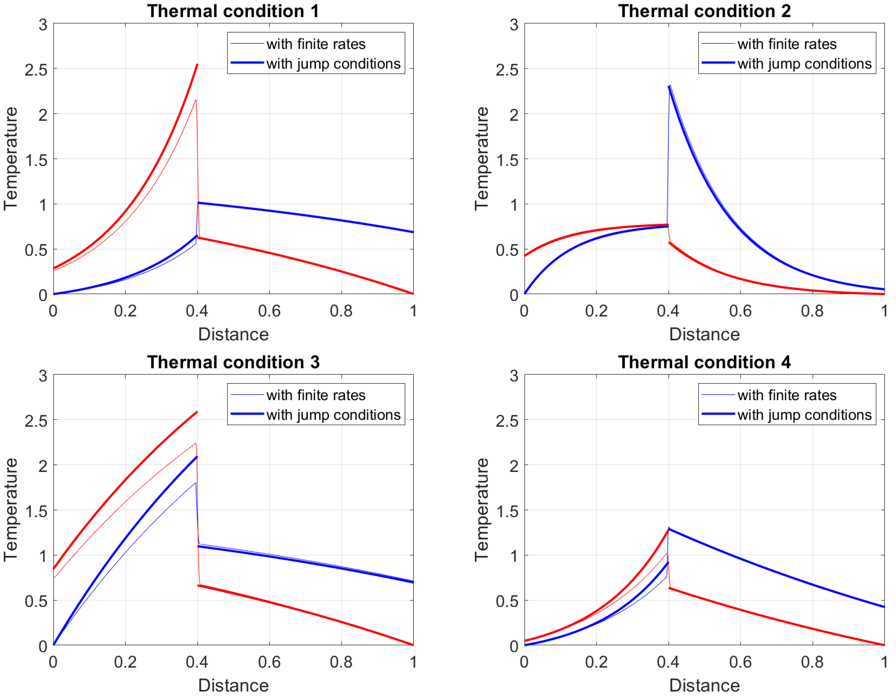
Figure 2.
Existence conditions for the four thermal cases as a function of the char concentration in the fuel and the air excess ratio . The black and the thin magenta lines correspond to and , respectively, while the think lines present the borders for the various thermal conditions. Plot (a) is representative of a , and Plot (b) is representative of .

Figure 3.
Typical temperature profiles expected in the counter current gasifier for . Pyrolysis is not present, and the reactor works under Thermal Condition 1 (a) and Thermal Condition 3 (b). The red lines indicate the temperature of the solid phase and the blue lines indicate the temperature of the gas phase.
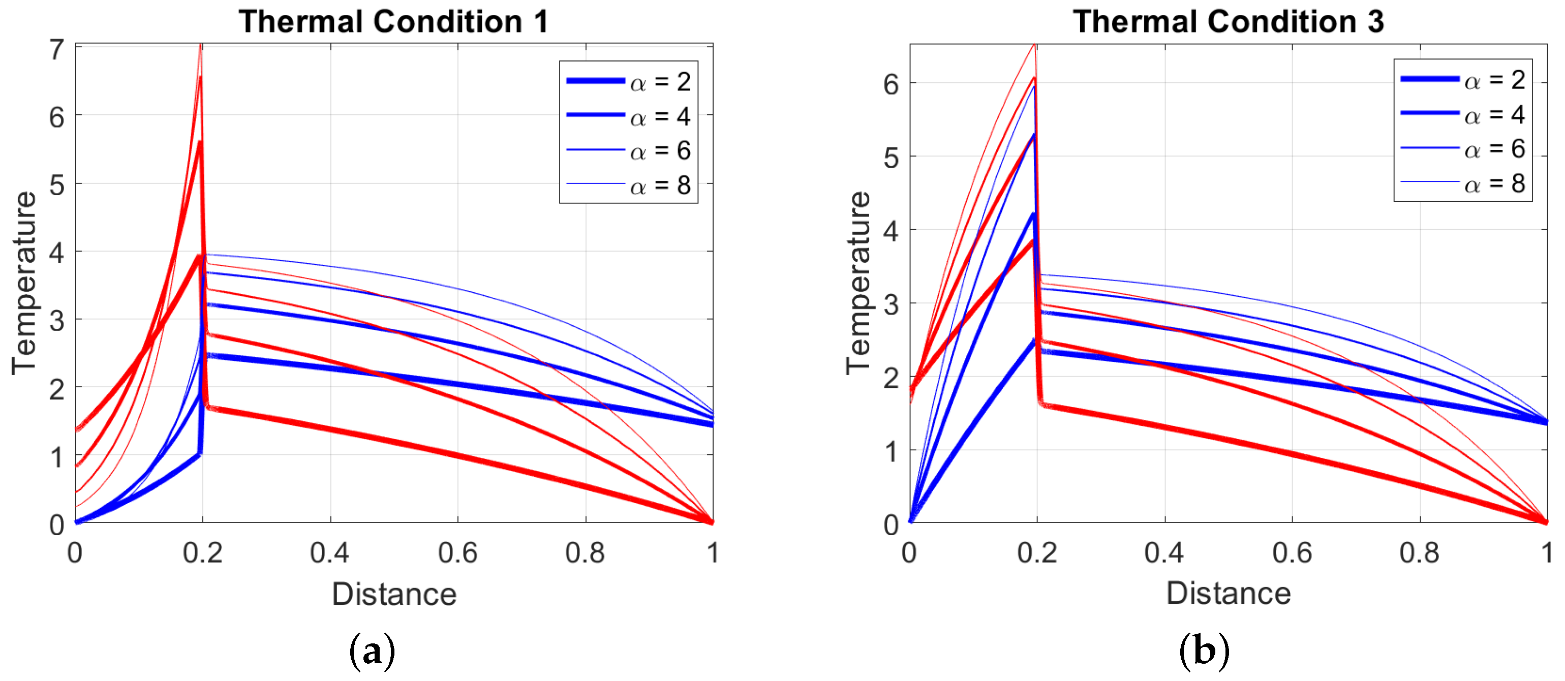
Figure 4.
Ignition temperature as a function of the position for the four thermal conditions. The curves are presented for four different values of the parameter and for different values of the parameter c.
Figure 4.
Ignition temperature as a function of the position for the four thermal conditions. The curves are presented for four different values of the parameter and for different values of the parameter c.
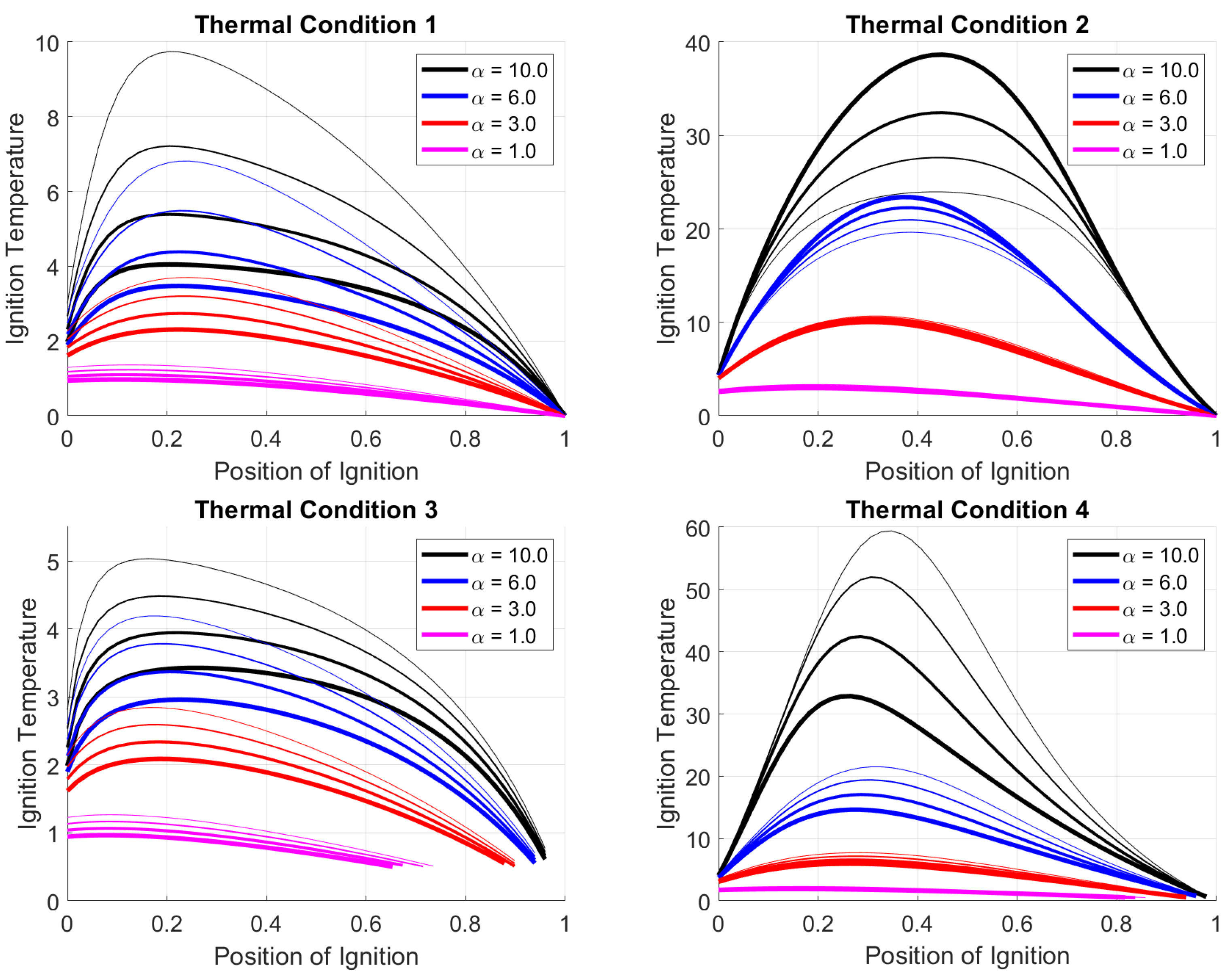
Figure 5.
Runaway position as a function of the non-dimensional fuel heating value q. (a) The plot on the left shows the runaway position for several parameters and constant , while (b) the plot on the right shows the runaway position for several ignition temperatures at a fixed thermal coupling . The thin lines are calculated with .

Figure 6.
Gas and solid phase temperature profiles for several reaction zones widths. The calculations have been performed in TC1. The blue lines show the gas temperature and the red lines the solid temperature.
Figure 6.
Gas and solid phase temperature profiles for several reaction zones widths. The calculations have been performed in TC1. The blue lines show the gas temperature and the red lines the solid temperature.

Figure 7.
The same as Figure 5 with a finite rate oxidation.
Figure 7.
The same as Figure 5 with a finite rate oxidation.

Figure 8.
(a) Solid temperature profiles and (b) char fraction profiles for different choices of the parameter . The calculation has been performed in TC1 and .
Figure 8.
(a) Solid temperature profiles and (b) char fraction profiles for different choices of the parameter . The calculation has been performed in TC1 and .
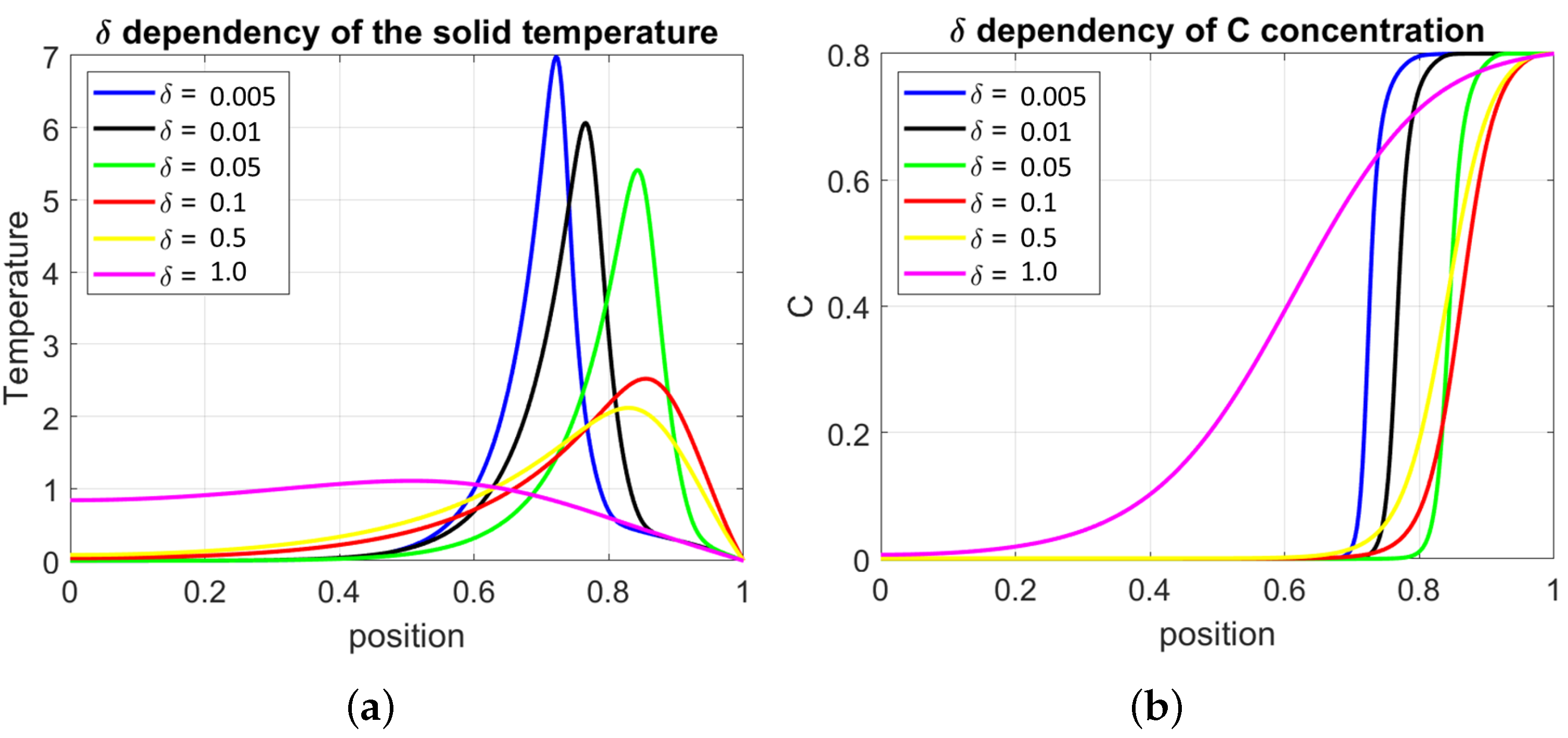
Figure 9.
Ignition temperature as a function of the position for the four cases when pyrolysis is present in the process. The other conditions are the same as for the calculations presented in Figure 4.
Figure 9.
Ignition temperature as a function of the position for the four cases when pyrolysis is present in the process. The other conditions are the same as for the calculations presented in Figure 4.

Figure 10.
Contour plot of the temperature in the space calculated with (a) (b) .

Figure 11.
Time variations of the solid temperature at the outlet ( in blue) and the maximal solid temperature (in red). (a) results for thermal coupling ; (b) results for thermal coupling .
Figure 11.
Time variations of the solid temperature at the outlet ( in blue) and the maximal solid temperature (in red). (a) results for thermal coupling ; (b) results for thermal coupling .
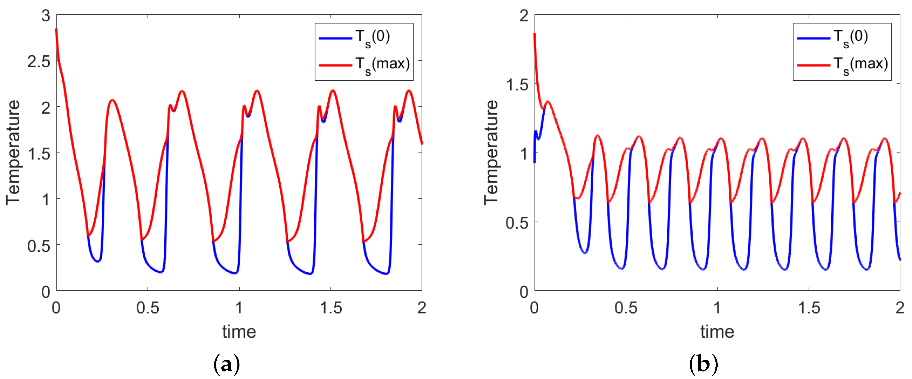
Figure 12.
Comparison between the ignition temperature in counter-current conditions (the magenta lines) and in co-flow conditions (the blue lines). The product is also shown.
Figure 12.
Comparison between the ignition temperature in counter-current conditions (the magenta lines) and in co-flow conditions (the blue lines). The product is also shown.
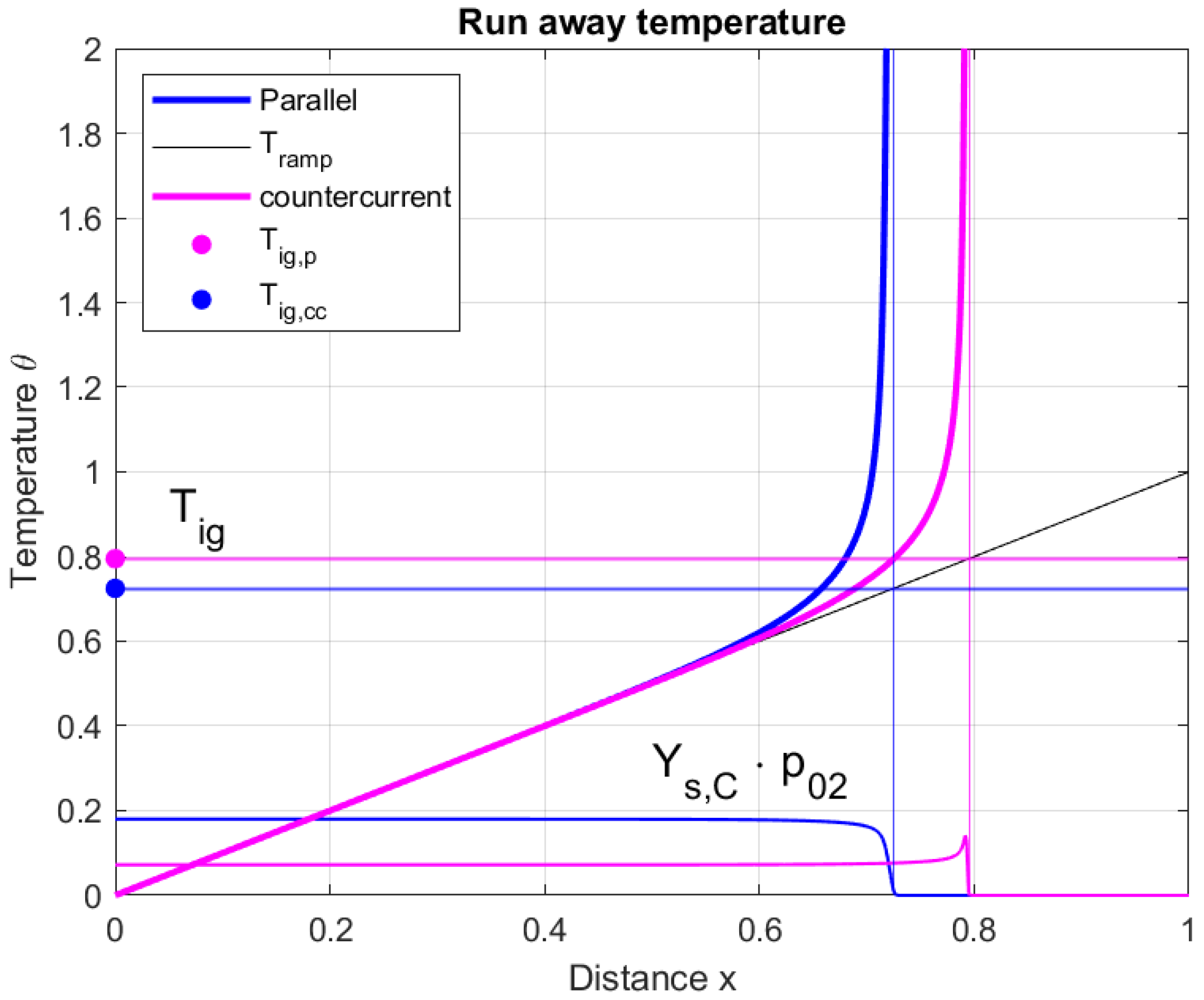
Figure 13.
Profiles of solid-phase Temperature (in red) and gas-pahse temperaturte (in blue) (a) of the MA process and (b) of the EL process. The thick lines are calculated with the flame front approximation while the thin lines are calculated with the finte rate model.
Figure 13.
Profiles of solid-phase Temperature (in red) and gas-pahse temperaturte (in blue) (a) of the MA process and (b) of the EL process. The thick lines are calculated with the flame front approximation while the thin lines are calculated with the finte rate model.
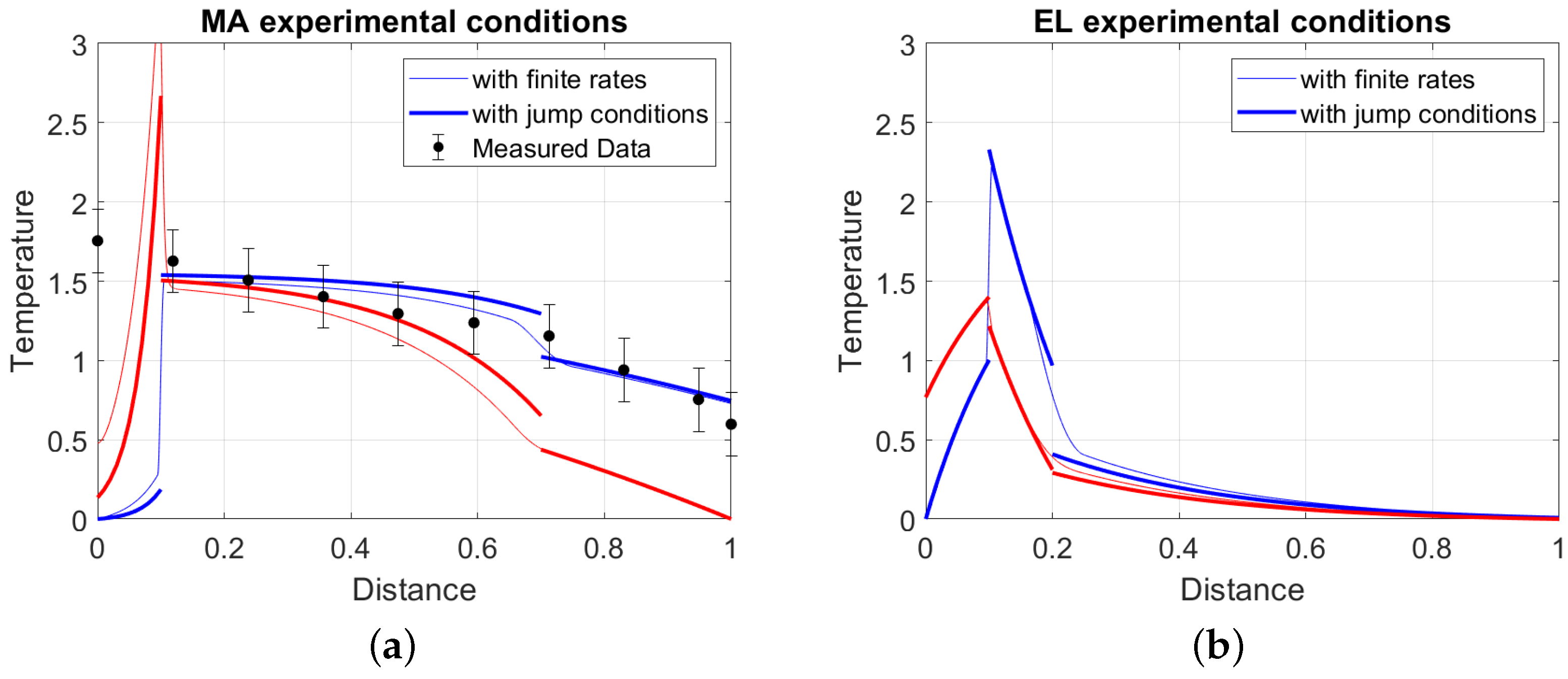
Figure 14.
Position of the Pyrolysis region as a function of the position of the combustion region for (a) the MA process and (b) for the EL process. The curves are calculated with four different thermal couplings (, the black, blue, rad and magenta lines respectively) and for the EL configuration and for the MA configuration.


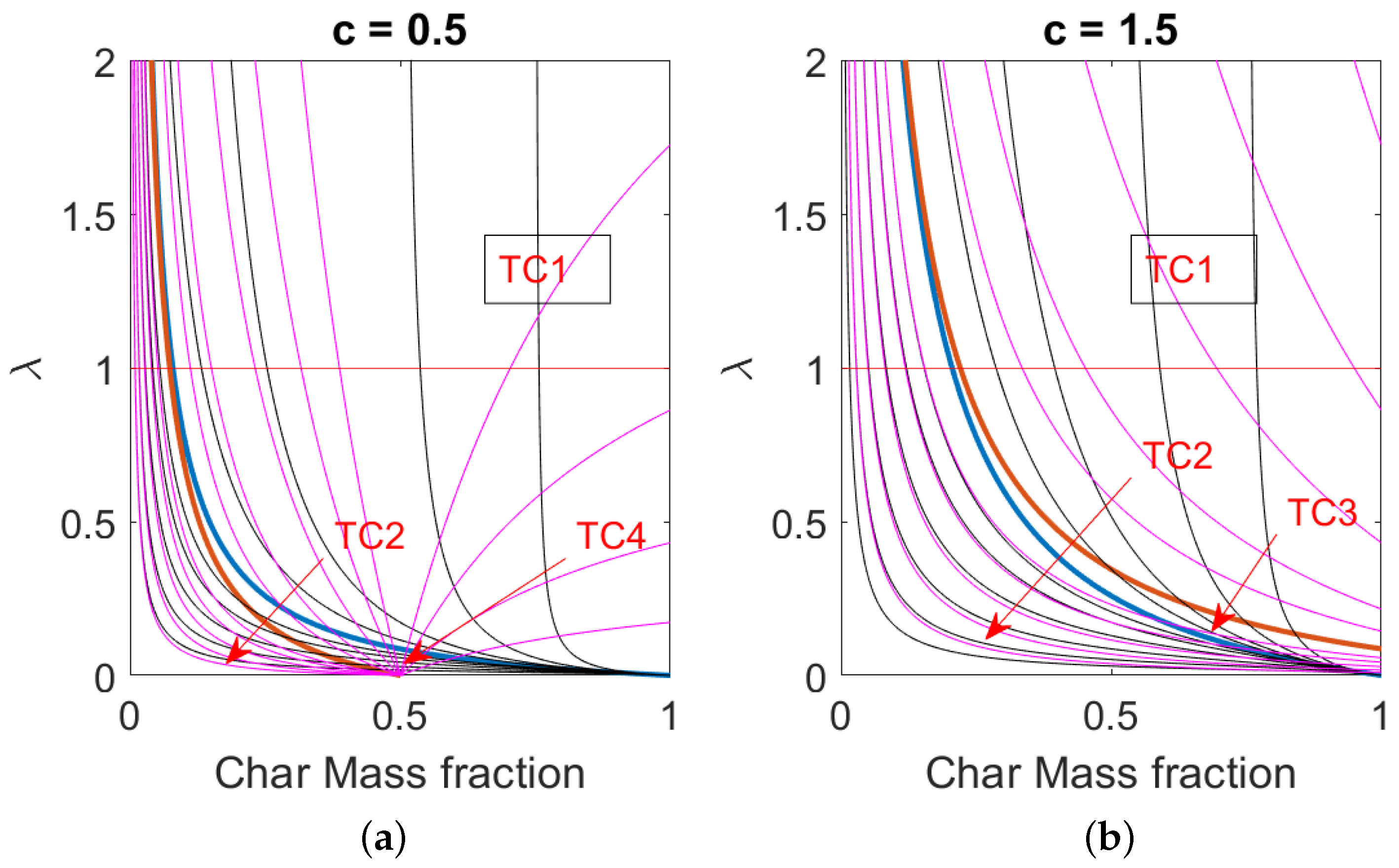
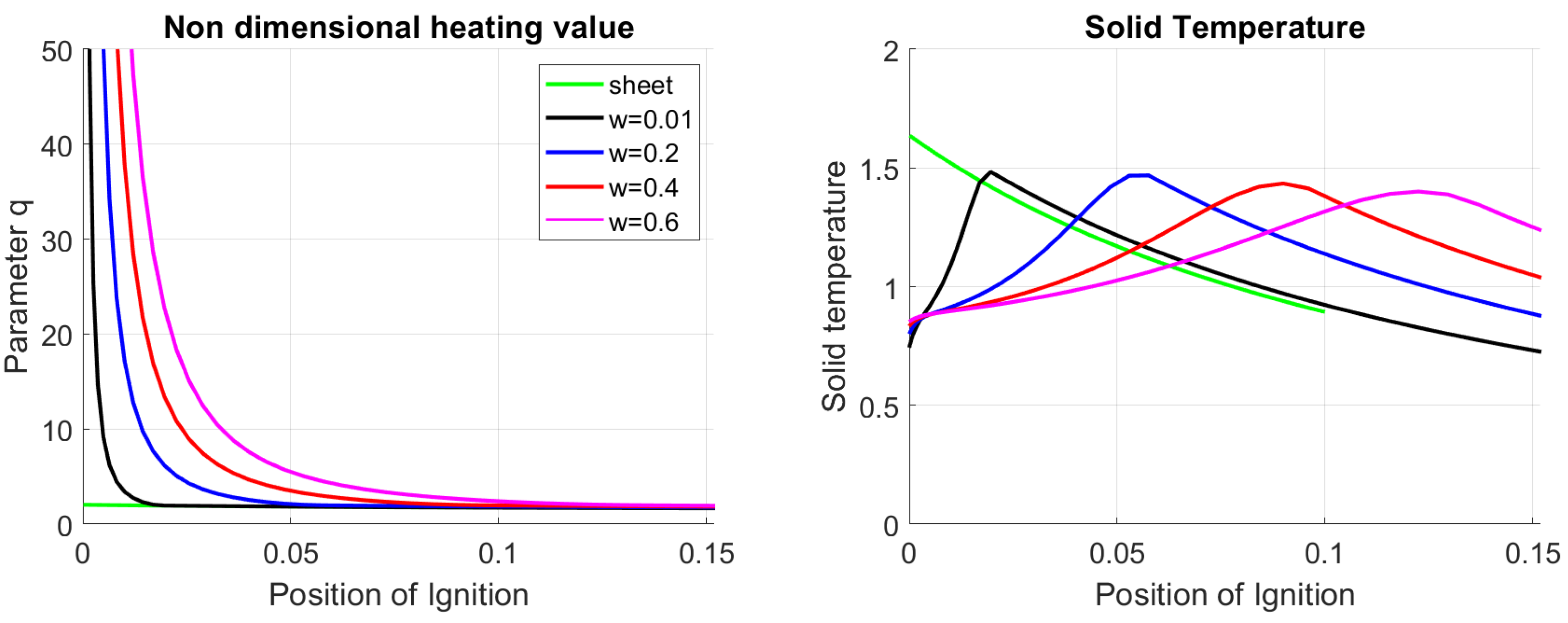
Table 1.
Values of the non-dimensional variables used for the simulation of the MA [30] and EL process [41].
| Oxidation | Pyrolysis | |||||||||||
|---|---|---|---|---|---|---|---|---|---|---|---|---|
| g | c | w | q | E | A | q | E | A | ||||
| EL process | ||||||||||||
| 9.0 | 2.2 | 0.9 | 1.98 | 0.06 | 15 | 10.8 | 0.14 | −3 | 6.5 | 400 | ||
| MA process | ||||||||||||
| 10 | 0.7 | 1.5 | 1.05 | 0.25 | 5 | 9.6 | 0.68 | −0.1 | 8.0 | 500 | ||
| Derived parameters | ||||||||||||
| Thermal case | w | |||||||||||
| EL | 0.73 | 0.78 | 0.54 | TC 2 | 1.25 | 1.20 | 1.44 | 1.98 | ||||
| MA | −13.2 | −0.52 | −0.6 | TC 1 | 14.25 | 1.37 | 1.63 | 1.05 | ||||
Table 2.
Parameters used in the calculation whose results are presented in Figure 4.
Table 2.
Parameters used in the calculation whose results are presented in Figure 4.
| TC 1 | TC 2 | TC 3 | TC 4 | |
|---|---|---|---|---|
| m | 0.4 | 0.4 | 0.4 | 0.4 |
| g | 1.6 | 1.6 | 8 | 1.6 |
| q | 4.0 | 4.0 | 4.0 | 4.0 |
| [10, 6, 3, 1] | ||||
| c | 0.8 | 2.3 | 0.6 | 2.3 |
| derived parameters | ||||
| 3.33 | 3.33 | 3.33 | 3.33 | |
| 2.12 | 2.12 | 6.60 | 2.12 | |
| w | 1.28 | 3.68 | 4.00 | 2.40 |
| −2.05 | 0.35 | 0.67 | −0.93 | |
| −0.84 | 1.56 | −2.60 | 0.28 | |
Disclaimer/Publisher’s Note: The statements, opinions and data contained in all publications are solely those of the individual author(s) and contributor(s) and not of MDPI and/or the editor(s). MDPI and/or the editor(s) disclaim responsibility for any injury to people or property resulting from any ideas, methods, instructions or products referred to in the content. |
© 2023 by the authors. Licensee MDPI, Basel, Switzerland. This article is an open access article distributed under the terms and conditions of the Creative Commons Attribution (CC BY) license (https://creativecommons.org/licenses/by/4.0/).
Share and Cite
MDPI and ACS Style
Mancini, M.; Schwabauer, A. On the Thermal Stability of a Counter-Current Fixed-Bed Gasifier. Energies 2023, 16, 3762. https://doi.org/10.3390/en16093762
AMA Style
Mancini M, Schwabauer A. On the Thermal Stability of a Counter-Current Fixed-Bed Gasifier. Energies. 2023; 16(9):3762. https://doi.org/10.3390/en16093762
Chicago/Turabian StyleMancini, Marco, and Andreas Schwabauer. 2023. "On the Thermal Stability of a Counter-Current Fixed-Bed Gasifier" Energies 16, no. 9: 3762. https://doi.org/10.3390/en16093762
Note that from the first issue of 2016, this journal uses article numbers instead of page numbers. See further details here.