Improving the Methodology for Determining the Biomass/Coal Co-Combustion Ratio: Predictive Modeling of the ¹⁴C Activity of Pure Biomass

Abstract

Sampling and ¹⁴C detection of biomass are now essential steps to ensure the accuracy of the ¹⁴C method, but they require additional time and economic investment. When there are multiple types of biomass fuels, it is not possible to guarantee the uniformity of sampling. The ¹⁴C activity of biomass fuels exhibits variability, and this value significantly impacts the precision of the ¹⁴C method. Therefore, this study aims to investigate the influencing factors of ¹⁴C activity in biomass fuels. It also provides predicted values of ¹⁴C activity for different types of biomass fuels for each year from 2020 to 2030. Additionally, this study discusses the potential blending ratio measurement errors that may arise due to the uncertainties of the predicted values. The reduction in the ¹⁴C activity of biomass fuels can occur due to the utilization of fossil fuels, human activities, and the photosynthesis mode of C3 plants. This study presents a prediction method for determining the reduction factor. The other component of the prediction methodology involves determining the original ¹⁴C activity of biomass fuels. The ¹⁴C activity of the annual biomass is equal to the ¹⁴CO₂ activity (the ¹⁴C activity of CO₂) of the surrounding environment, and it experiences a decline of 0.355 pMC/year. The ¹⁴C activity has ranges of five types of perennial biomass fuels, including wood chips and branches, bark, leaves, wasted furniture, and abandoned building wood, for the time period between 2020 and 2030, are 97.34~102.84, 96.35~106.27, 96.35~102.64, 111.00~118.60, and 111.32~129.47 pMC, respectively. Based on these, this study introduces a new formula for calculating blending ratios, which enhances the current methodology. The calculation errors of blending ratios caused by the uncertainties of the predicted values are generally negligible, with the exception of wasted furniture and construction wood. The annual decrease in the blending ratio calculation error, caused by the uncertainty associated with the predicted value, can be observed. This study aims to reduce the implementation time and economic cost of the ¹⁴C method while ensuring the accuracy of biomass blending ratio detection.

1. Introduction

Biomass–coal co-firing power generation technology has been identified as an effective approach to facilitate the achievement of “carbon peaking and neutrality” [1] and the utilization of biomass resources [2,3,4]. Currently, a significant amount of research has been dedicated to accurately determining the biomass/coal co-firing blending ratio [5,6,7]. This is performed in order to establish a foundation for the precise calculation of carbon emission reduction.

Among the various methods available, the ¹⁴C method is widely regarded as having the highest potential for accurately determining the blending ratio [8]. The ¹⁴C method is utilized to quantitatively measure the proportion of biogenic fuels, which contain a specific concentration of ¹⁴C, to fossil fuels, where the radiocarbon has completely decayed. This is achieved by analyzing the ¹⁴CO₂ activity in the flue gas [9,10]. The ¹⁴C activity is the percentage ratio of the ¹⁴C/¹²C value in the substance to the ¹⁴C/¹²C value in the international standard reference material (oxalic acid). In this particular process, the ¹⁴C activity of pure biomass is utilized as the reference value in the calculation formula, as demonstrated in Equation (1), and it significantly influences the accuracy of the calculation results [5]. The conventional method for obtaining this reference value, in order to ensure the accuracy of the co-firing blending ratio calculation results, typically involves the sampling -¹⁴C detection process of the biomass fuels combusted in furnaces [11]. Alternatively, some standards recommend using the ¹⁴C activity of the current atmospheric CO₂ as a predictor of the ¹⁴C activity of biomass fuels [12]. Biomass is continually undergoing photosynthesis and respiration during its growth cycle, and the carbon in its body is derived from CO₂ in the air. Due to the carbon exchange cycle, the ¹⁴C activity of biomass should theoretically be equal to the ¹⁴C activity of atmospheric CO₂. However, it is important to note that the actual value may deviate from this theoretical expectation, either increasing or decreasing, due to various influencing factors.

$${\mathrm{f}}_{\mathrm{b}\mathrm{i}\mathrm{o}\mathrm{m}\mathrm{a}\mathrm{s}\mathrm{s}}^{\mathrm{c}\mathrm{b}}=\frac{{\mathrm{A}}_{\mathrm{f}\mathrm{l}\mathrm{u}\mathrm{e}\mathrm{g}\mathrm{a}\mathrm{s}}-{\mathrm{A}}_{\mathrm{N}\mathrm{a}\mathrm{O}\mathrm{H}}\times {\mathrm{f}}_{\mathrm{N}\mathrm{a}\mathrm{O}\mathrm{H}}^{\mathrm{c}\mathrm{b}}}{{\mathrm{A}}_{\mathrm{b}\mathrm{i}\mathrm{o}\mathrm{m}\mathrm{a}\mathrm{s}\mathrm{s}}}\times 100\%$$

(1)

where ${\mathrm{f}}_{\mathrm{b}\mathrm{i}\mathrm{o}\mathrm{m}\mathrm{a}\mathrm{s}\mathrm{s}}^{\mathrm{c}\mathrm{b}}$ and ${\mathrm{A}}_{\mathrm{b}\mathrm{i}\mathrm{o}\mathrm{m}\mathrm{a}\mathrm{s}\mathrm{s}}$ are the carbon-based blending ratio and the ¹⁴C activity of biomass, respectively. ${\mathrm{A}}_{\mathrm{f}\mathrm{l}\mathrm{u}\mathrm{e}\mathrm{g}\mathrm{a}\mathrm{s}}$ and ${\mathrm{A}}_{\mathrm{N}\mathrm{a}\mathrm{O}\mathrm{H}}\times {\mathrm{f}}_{\mathrm{N}\mathrm{a}\mathrm{O}\mathrm{H}}^{\mathrm{c}\mathrm{b}}$ are the ¹⁴C activity of CO₂ in flue gas absorbed by NaOH.

The ¹⁴C activity of biomass is subject to various factors, including the growth cycle, growth location, and biomass types. The atmospheric ¹⁴CO₂ activity remained in a state of dynamic equilibrium with minor fluctuations around 100 pMC until the 1960s. However, the frequent nuclear explosion tests conducted during this period resulted in a nearly twofold increase in the atmospheric ¹⁴CO₂ activity [13]. The significant utilization of fossil fuels during the later period has resulted in a decline in the atmospheric ¹⁴CO₂ activity. This decline has continued in recent years at a rate of 0.3 to 0.5 pMC/year [14]. Figure 1 illustrates the ¹⁴C activity of the atmospheric background in the northern hemisphere, spanning the years 1920 to 2019. For annual agricultural waste, such as straw, in recent years, it has been observed that the predicted ¹⁴C activity closely approximates the ¹⁴C activity of the atmospheric background for that specific year [15,16]. However, the ¹⁴C activity of perennial biomass, especially wood board, which undergoes growth cycles that may be influenced by fluctuations in atmospheric ¹⁴CO₂ activity, exhibits significant variability [11,12,17,18]. This is the influence of the growth cycle and types on the ¹⁴C activity of biomass. Another aspect to consider regarding the impact of biomass types is the potential for varying photosynthesis patterns, which can cause slight isotopic fractionation. This, in turn, can lead to notable disparities in the ¹⁴C activities of C3 and C4 biomass [19]. Moreover, in certain regions, the extensive utilization of fossil fuels and human-induced activities may lead to a decrease in the local ¹⁴CO₂ activity compared to the atmospheric background ¹⁴CO₂ activity, and this reduction can result in a decrease in the ¹⁴C activity of biomass within that specific area [20,21]. The aforementioned statement highlights the impact of growth location on the ¹⁴C activity of biomass.

Previous studies have examined the prediction of ¹⁴C activity in pure biomass, considering various influencing factors. Fellner [12] and Mohn [18] provided the predicted value of ¹⁴C activity for biogenic fractions in waste power plants in 2008 and 2009. However, this value was only applicable to the biomass fraction in waste and solid recovered fuels, and the predicted year is no longer relevant today. Tang [11] proposed a formula to predict the ¹⁴C activity of biomass fuels in biomass–coal co-combustion power plants. However, the study lacked sufficient investigation into factors such as the growth cycle. Biomass fuels used in power plants come from a variety of sources, making it difficult to obtain accurate ¹⁴C activity reference values through sampling and testing. This process also incurs additional time and economic costs. Furthermore, when government departments visit power plants to monitor biomass blending ratios, they are not permitted to conduct uniform sampling of biomass fuels and ¹⁴C testing due to time constraints. Therefore, conducting a comprehensive study on various influencing factors is crucial for accurately predicting ¹⁴C activity values for different biomass fuels in the future. This is essential for the effective application of the ¹⁴C method in industrial power plants.

In this study, we conducted a detailed investigation of the various factors influencing the ¹⁴C activity of biomass fuel in biomass and coal-coupled combustion power plants. This involved sampling, ¹⁴C detection, calculation, and other methods. Additionally, we proposed an innovative prediction model for the ¹⁴C activity of biomass in co-combustion power plants. The proposed calculation method can eliminate the need for sampling, sample preparation, and the ¹⁴C detection of biomass fuel in the ¹⁴C method. This can significantly improve the timeliness and cost effectiveness of the ¹⁴C method and provide a great convenience for government testing departments to monitor biomass blending ratios in real time. We investigate the effects of the growth cycle, growth location, and biomass type in order to develop this method. The anticipated ¹⁴C activity levels of yearly biomass, wood chips, bark, branches, leaves, waste furniture, and construction wood were also computed for each year spanning from 2020 to 2030. This study addresses the requirement for the optimal and rational utilization of the ¹⁴C method in industrial power plants. Furthermore, the advancement of the ¹⁴C methodology has facilitated the widespread adoption and advancement of biomass energy utilization technologies, leading to a reduction in the reliance on fossil fuels and contributing to sustainable socio-economic development.

2. Materials and Methods

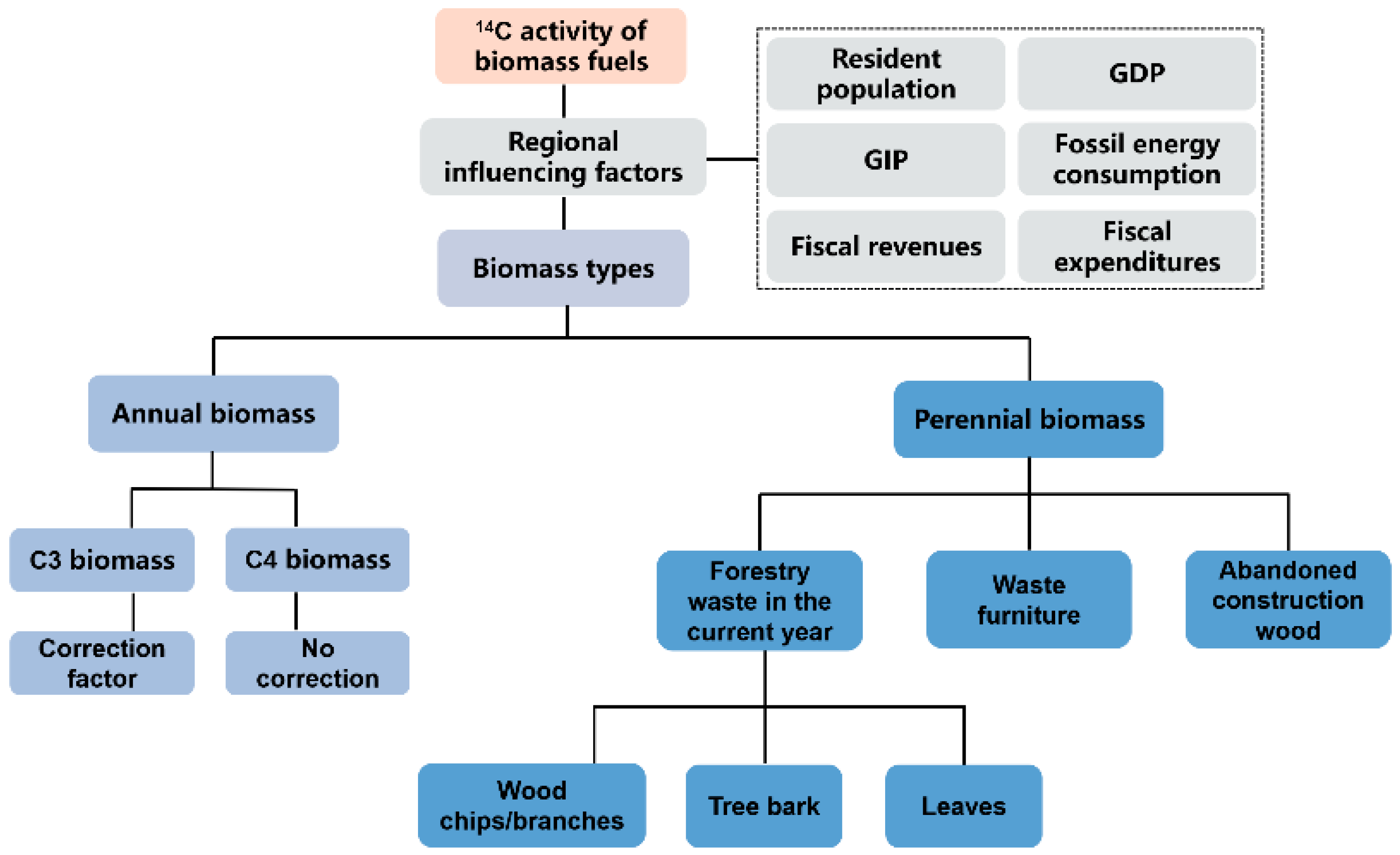
2.1. Biomass Classification

In the present study, the classification of biomass fuels was conducted, distinguishing between annual biomass and perennial biomass. Among the various types of biomasses, the annual biomass consists of C3 plants, such as wheat straw and rice straw, as well as C4 plants, which are represented by corn straw. Plants that initially produce the four-carbon compound malic acid or aspartate instead of the three-carbon compound 3-phosphoglyceric acid in the photosynthetic carbon cycle are called C4 plants. Plants that initially produce 3-phosphoglyceric acid are called C3 plants. Perennial biomass encompasses various forms of organic waste, such as forestry residues (wood chips, branches, bark, and leaves), as well as wasted furniture wood and construction wood, commonly known as wood board.

2.2. Sampling and Processing

2.2.1. Tree Ring Samples

Tree rings, which exhibit annual growth patterns, serve as the most accurate indicators of atmospheric ¹⁴CO₂ levels within a given year. In this study, the rings of camphor trees were sampled from ten cities in Zhejiang Province, China, including Hangzhou, Ningbo, Jinhua, Quzhou, Wenzhou, Lishui, Taizhou, Jiaxing, Shaoxing, and Huzhou. The sampling sites were all in the suburbs far from the main urban area, and there were no highways within 1 km and no residential houses within 100 m. The objective was to examine the influence of regional factors on atmospheric ¹⁴CO₂ activity in different locations. This was achieved by analyzing data from various economic indicators of each city and combining them with the ¹⁴C activity of the collected tree ring samples. Following the collection process described by Hou [20], representative samples of tree rings were obtained for each city’s atmospheric ¹⁴CO₂ activity in 2019.

2.2.2. C3 Plants Samples

In this paper, the most typical C3 biomass fuels, wheat straw and rice straw, were selected for this study. Wheat straw and rice straw were collected from two townships in Pingdingshan, China, and two townships in Hangzhou, China, respectively, at the maturity of the wheat and rice. The two sampling points in Pingdingshan were Wangping Village and Guangtian Township, and the two sampling points in Hangzhou were Linjiang Village and Hongdong Village. While the straw samples were collected, air carbon dioxide was collected from the field at different times of the day for the subsequent comparison of the ¹⁴C activity of CO₂ and straw samples. The sampling point of carbon dioxide is within 3 m of the sampling point of straw. The air was passed through two 1 mol/L NaOH solutions at a flow rate of 4 L/min to absorb CO₂ from the air. After being absorbed, the NaCO₃ solution was converted into SrCO₃ precipitation for the purpose of subsequent sample preparation and testing. The carbon in SrCO₃ comes from atmospheric CO₂.

2.2.3. ¹⁴C Sample Preparation and Detection

A high-vacuum graphitization synthesis system, comprising a high-vacuum ion pump and a high-vacuum reactor, was employed to transform the tree rings, straw, and air CO₂ samples into graphite [5,7,11]. The preparation process of graphite samples includes oxidation combustion and catalytic reduction. The graphite samples were submitted to an accelerator mass spectrometry facility for the purpose of detecting their ¹⁴C activities.

2.3. Data Acquisition

This study collected data on various variables, including the resident population, gross regional product (GDP), gross industrial product (GIP), fossil energy consumption, fiscal revenue, and fiscal expenditure, for dozens of cities in different years. The data were partially obtained from the yearbooks of each city, including nine districts in Beijing in 2009 [24], fifteen cities in 2010 [25,26,27,28,29,30,31,32,33,34,35,36,37,38,39], five cities in 2014 [40,41,42,43,44], and ten cities in Zhejiang Province in 2019 [45,46,47,48,49,50,51,52,53,54]. Furthermore, previous studies have gathered atmospheric ¹⁴C activity data for specific years in various cities throughout the country [15,55,56,57,58]. These data sources were utilized to establish a solid foundation for the examination of regional influencing factors.

The prediction of ¹⁴C activity in perennial biomass necessitates the utilization of growth function models specific to each tree species. In this study, a total of 14 commonly found tree species were selected for analysis. The subsequent sections will discuss the growth function models for these species.

2.4. Prediction Method

2.4.1. Regional Influencing Factors

In this study, the standard equation method was used to resolve the linear fitting equations of the six economic indicators of a specific region with respect to the reduction factor of atmospheric ¹⁴CO₂ activity ($\mathrm{R}\mathrm{F}$, defined as the ratio of the atmospheric ¹⁴CO₂ activity at the site to the ¹⁴CO₂ activity of the northern hemisphere atmospheric background in the current year), as shown in the subsequent equation:

$$\mathrm{R}\mathrm{F}={\mathrm{a}}_0+{\mathrm{a}}_1\times {\mathrm{x}}_1+{\mathrm{a}}_2\times {\mathrm{x}}_2+{\mathrm{a}}_3\times {\mathrm{x}}_3+{\mathrm{a}}_4\times {\mathrm{x}}_4+{\mathrm{a}}_5\times {\mathrm{x}}_5+{\mathrm{a}}_6\times {\mathrm{x}}_6$$

(2)

where ${\mathrm{x}}_1$~${\mathrm{x}}_6$ are the economic indicator data of each city in the dataset and ${\mathrm{a}}_0$~${\mathrm{a}}_6$ are the fitting coefficients in front of each variable of the linear equation. The dataset includes data from previous studies and data from 10 cities in Zhejiang Province obtained by this study. The dataset is divided into training sets and test sets.

$$\mathrm{J}({\mathrm{a}}_0,{\mathrm{a}}_1,{\mathrm{a}}_2,{\mathrm{a}}_3,{\mathrm{a}}_4,{\mathrm{a}}_5,{\mathrm{a}}_6)=\frac{1}{2\mathrm{m}}\times {\displaystyle \sum _{\mathrm{i}=1}^{\mathrm{m}}{({\mathrm{h}}_{\mathrm{a}}({\mathrm{x}}^{(\mathrm{i})})-\mathrm{R}{\mathrm{F}}^{(\mathrm{i})})}^2}$$

(3)

Equation (3) defines the cost function ($\mathrm{J}({\mathrm{a}}_0,{\mathrm{a}}_1,{\mathrm{a}}_2,{\mathrm{a}}_3,{\mathrm{a}}_4,{\mathrm{a}}_5,{\mathrm{a}}_6)$) for fitting the equation, i.e., the average value of the residuals of each array in the training set. ${\mathrm{h}}_{\mathrm{a}}({\mathrm{x}}^{(\mathrm{i})})$ and $\mathrm{R}{\mathrm{F}}^{(\mathrm{i})}$ are the fitting value and actual value of the reduction factor. Our aim is to fit a suitable ${\mathrm{a}}_0$~${\mathrm{a}}_6$ that minimizes the value of this cost function. Since the image model of this cost function contains only one extreme point, the ${\mathrm{a}}_0$~${\mathrm{a}}_6$ corresponding to the position of this extreme point is the prediction result. Define matrix $\mathrm{X}$, $\mathrm{R}\mathrm{F}$, and $\mathsf{\omega }$ as the matrix composed of each city’s economic indicators, reduction factor, and ${\mathrm{a}}_0$~${\mathrm{a}}_6$, respectively, and then there is the following formula to find the matrix $\mathsf{\omega }$. ${\mathrm{X}}^{\mathrm{T}}$ is the transpose of $\mathrm{X}$.

$$\mathrm{J}({\mathrm{a}}_0,{\mathrm{a}}_1,{\mathrm{a}}_2,{\mathrm{a}}_3,{\mathrm{a}}_4,{\mathrm{a}}_5,{\mathrm{a}}_6)=\frac{1}{2\mathrm{m}}\times {(\mathrm{R}\mathrm{F}-\mathrm{X}\mathsf{\omega })}^{\mathrm{T}}\times (\mathrm{R}\mathrm{F}-\mathrm{X}\mathsf{\omega })$$

(4)

$$\frac{\partial }{\partial {\mathsf{\alpha }}_{\mathrm{j}}}\mathrm{J}(\mathrm{a})=0$$

(5)

$$\mathsf{\omega }={({\mathrm{X}}^{\mathrm{T}}\mathrm{X})}^{-1}{\mathrm{X}}^{\mathrm{T}}\mathrm{R}\mathrm{F}$$

(6)

2.4.2. Annual Biomass

C3 plants are a classification of plants that produce a three-carbon compound called 3-phosphoglyceric acid as their initial product of CO₂ assimilation in the photosynthetic carbon cycle. Certain plants undergo isotopic fractionation to a certain extent when they absorb CO₂ from the atmosphere. This process leads to a reduction in their own ¹⁴C activity in comparison to the ¹⁴CO₂ activity in the surrounding air. This study was based on the isotope fractionation correction method [59] and aimed to forecast the degree of variation in the ¹⁴C activity of C3 plants compared to atmospheric CO₂. ¹³C is a kind of stable isotope of carbon. ¹³C content refers to the value of ¹³C/¹²C of the substance. This was achieved by utilizing the difference in ¹³C content (expressed in thousandths of a percent) between C3 plants and air CO₂, as shown in the subsequent equation:

$$\frac{{}^{14}\mathrm{C}_{\mathrm{N}}}{{}^{14}\mathrm{C}}={(\frac{{}^{13}\mathrm{a}_{\mathrm{N}}}{{}^{13}\mathrm{a}})}^{\mathsf{\theta }}={(\frac{1+{}^{13}\mathsf{\delta }_{\mathrm{N}}}{1+{}^{13}\mathsf{\delta }})}^{\mathsf{\theta }}$$

(7)

where the numerator is the correlation value of C3 plants, which is equal to the corrected value, while the denominator term is the correlation value of air CO₂, which is equal to the pre-corrected value. In this study, four sets of data obtained from the four sampling sites were fitted to the value of the correction parameter $\mathsf{\theta }$, and then we can calculate the degree of deviation of the ¹⁴C activity of C3 plants relative to the atmospheric CO₂ in each location using the ${}^{13}\mathsf{\delta }$ values of C3 plants and air CO₂. This is a more accurate way of correcting for the ¹⁴C activity of annual C3 biomass. ${}^{13}\mathrm{a}$ and ${}^{13}\mathsf{\delta }$ represent the ¹³C activity value and its thousandth difference from the standard matter.

2.4.3. Perennial Biomass

Based on previous studies [12], the average ¹⁴C activity of perennial plants is calculated according to the following equation:

$${}^{14}\mathrm{C}=\frac{{\displaystyle {\int }_{{\mathrm{t}}_1}^{{\mathrm{t}}_2}\mathrm{p}\mathrm{M}\mathrm{C}(\mathrm{t})\times \frac{\mathrm{d}\mathrm{V}}{\mathrm{d}\mathrm{t}}\mathrm{d}\mathrm{t}}}{{\displaystyle {\int }_{{\mathrm{t}}_1}^{{\mathrm{t}}_2}\frac{\mathrm{d}\mathrm{V}}{\mathrm{d}\mathrm{t}}\mathrm{d}\mathrm{t}}}$$

(8)

$\mathrm{V}$ is the growth function model of the plant and $\mathrm{p}\mathrm{M}\mathrm{C}(\mathrm{t})$ is the atmospheric ¹⁴C activity in the corresponding year. $\mathrm{t}$ is the age of the plant. The growth function represents the relationship between plant volume and age. The harvesting age refers to the stage in the plant’s growth when it reaches the cutting standard. In this study, the growth function models for 14 different tree species were initially gathered. The common plant growth function is presented in Table S1, and the growth model functions for these trees are presented in

Table 1. The growth function models of fourteen kinds of trees.

Tree Types	Growth Function	Harvesting Age
Eucalyptus	$\mathrm{V}(\mathrm{t})=\frac{0.07965}{1+\exp (2.7076-0.8577\times \mathrm{t})}$	6~10
Cypress	$\mathrm{V}(\mathrm{t})=0.01927\times {[1-0.98444\times \exp (-0.08419\times \mathrm{t})]}^{4.52246}$	40~50
Sassafras	$\mathrm{V}(\mathrm{t})=0.725806\times {[1-\exp (-0.07412\times \mathrm{t})]}^{5.205163}$	20~50
Birch	$\mathrm{V}(\mathrm{t})=\frac{0.91692}{1+\exp (5.41257-0.17846\times \mathrm{t})}$	15~50
Oak	$\mathrm{V}(\mathrm{t})=0.7013\times {[1-\exp (-0.0334\times \mathrm{t})]}^{5.2521}$	50~100
Willow	$\mathrm{V}(\mathrm{t})=1.55274\times {[1-3.18331\times \exp (-0.40973\times \mathrm{t})]}^{3.04096}$	15~20
Cedar	$\mathrm{V}(\mathrm{t})=0.210524\times {[1-0.7323\times \exp (-0.02487\times \mathrm{t})]}^{5.16562}$	20~40
Pinus Massoniana	$\mathrm{V}(\mathrm{t})=0.35833\times {[1-\exp (-0.04606\times \mathrm{t})]}^{5.22947}$	25~40
Chinese Red Pine	$\mathrm{V}(\mathrm{t})=\frac{0.166}{1+216.656\times \exp (-0.164\times \mathrm{t})}$	30~60
Larch	$\mathrm{V}(\mathrm{t})=\frac{0.045}{1+1035.485\times \exp (-0.407\times \mathrm{t})}$	30~40
Camphor	$\mathrm{V}(\mathrm{t})=\frac{1.1768}{1+50.4297\times \exp (-0.0907\times \mathrm{t})}$	30~80
Poplar	$\mathrm{V}(\mathrm{t})=0.5483\times {[1-\exp (-0.1848\times \mathrm{t})]}^{3.9547}$	10~20
Beech	$\mathrm{V}(\mathrm{t})=\mathrm{A}\times {[1-\exp (0.0333-0.0167\times \mathrm{t})]}^2$	50~100
Locust	$\mathrm{V}(\mathrm{t})=0.41129\times {[1-\exp (-0.03468\times \mathrm{t})]}^{1.54264}$	10~60

. Additionally, the age at which each tree reaches maturity, also known as the age at felling, is provided in the table. The growth patterns exhibited by the majority of tree species adhered to the Chapman–Richard and Logistic models. Subsequently, the average ¹⁴C activity of trees at various ages, which were harvested each year, was individually calculated. The ¹⁴C activity prediction values for wood chips and branches were determined by selecting the average values of the ¹⁴C activity from the harvested trees within the specified age range. For the analysis of bark and leaves, it is necessary to establish prediction values based on the annual renewal cycles of these tree components. Wood board fuels primarily derive from discarded furniture and abandoned construction wood, with an average lifespan of 10~30 years and 50~60 years. Therefore, the wood board fuels that were harvested in a specific year were actually cut down several decades ago. Both the service life and the age at which the tree is cut down are considered in the prediction process. For instance, the year of the felling of waste poplar furniture in 2023 should fall within the range of 1993 and 2013. Within this range, the ¹⁴C activity of poplar at each harvesting age, corresponding to each felling year, represents an average term of the predicted value.

2.5. Improved Methodology

Based on the prediction of ¹⁴C activity of various types of biomasses, the following equation was proposed in this study for the calculation of the biomass/coal co-combustion blending ratio:

$${\mathrm{f}}_{\mathrm{b}\mathrm{i}\mathrm{o}\mathrm{m}\mathrm{a}\mathrm{s}\mathrm{s}}^{\mathrm{c}\mathrm{b}}=\frac{{\mathrm{A}}_{\mathrm{f}\mathrm{l}\mathrm{u}\mathrm{e}\mathrm{g}\mathrm{a}\mathrm{s}}-{}^{14}\mathrm{C}_{\mathrm{air}}\times {\mathrm{f}}_{\mathrm{a}\mathrm{i}\mathrm{r}}^{\mathrm{c}\mathrm{b}}}{{\displaystyle \sum _{\mathrm{i}=1}^{\mathrm{n}}{}^{14}\mathrm{C}_{\mathrm{pre\_i}}\times {\mathrm{f}}_{\mathrm{f}\mathrm{u}\mathrm{e}\mathrm{l}\_\mathrm{i}}}}\times 100\%$$

(9)

where ${}^{14}\mathrm{C}_{\mathrm{pre\_i}}$ is the prediction value of the ¹⁴C activity of different types of biomass fuel and ${\mathrm{f}}_{\mathrm{f}\mathrm{u}\mathrm{e}\mathrm{l}\_\mathrm{i}}$ is the carbon-based percentage of the biomass fuel. The specific calculations will be described in subsequent chapters. ${\mathrm{A}}_{\mathrm{f}\mathrm{l}\mathrm{u}\mathrm{e}\mathrm{g}\mathrm{a}\mathrm{s}}$ is the ¹⁴C activity of flue gas CO₂. ${}^{14}\mathrm{C}_{\mathrm{air}}\times {\mathrm{f}}_{\mathrm{a}\mathrm{i}\mathrm{r}}^{\mathrm{c}\mathrm{b}}$ represents the ¹⁴C activity originated from the air CO₂. Unlike the traditional ¹⁴C calculation formula (such as Equation (1)), the ¹⁴C activity value of biomass in the denominator of this formula is not obtained through actual detection but is a predicted value based on the research results in this paper. This approach eliminates the need for sampling and the ¹⁴C detection of biomass fuel, improving the timeliness and cost effectiveness of the ¹⁴C method while ensuring accuracy. In addition, when there are multiple types of biomass fuels in the power plant, achieving uniform sampling becomes challenging. Predicting the ¹⁴C activity of biomass can provide a quick way to determine the blending ratio.

3. Results and Discussion

3.1. Regional Influencing Factors

3.1.1. Fitting Results at the City Level

The research results in this section are based on the city as the smallest unit. Figure 2 illustrates the correlation between atmospheric ¹⁴CO₂ activity and various socio-economic factors, including the number of residents, GDP, GIP, fossil energy consumption, fiscal revenue, and fiscal expenditure, in ten cities located in Zhejiang Province in the year 2019. These data were obtained through the tree ring sample -¹⁴C detection process conducted in this study. Similar to the findings of previous research [15], there is a tendency for the atmospheric ¹⁴CO₂ activity in a given region to exhibit a negative correlation with the level of economic development in that region. Hangzhou and Ningbo, being the two most prominent cities in Zhejiang Province, exhibit the lowest levels of atmospheric ¹⁴CO₂ activity. The level of fossil energy consumption exhibits a significant negative correlation (R² = 0.885), making it the primary factor responsible for the decline in atmospheric ¹⁴CO₂ activity. Since only 10 cities’ tree rings were sampled in this study, which may be under-representative, multiple sets of data from other studies were used in the fitting at the same time, encompassing different cities and different years, to make it more statistically representative. The findings of previous research [15,21,57,58] demonstrate consistent outcomes, as depicted in Figures S1 and S2. These figures illustrate the correlation between the reduction factor of atmospheric ¹⁴C activity and local economic indicators in various cities nationwide in 2010 and 2014, respectively. In the present study, the standard equation method, as described in Section 2.4.1, was employed to perform linear regression analysis on a dataset comprising data from 27 cities (refer to Figure 1, Figures S1 and S2). The test set for detecting the relative errors of the prediction results consisted of data from four cities: Jiuquan, Yantai, Hangzhou, and Lishui.

The results of the prediction are presented in Table 1. To compare the fitting results of various factors, the statistical software SPSS 26.0 was employed to analyze the correlation among these factors. The analysis revealed that fossil energy consumption, the number of resident populations, and the GDP exhibited the highest level of significance, while the remaining three factors demonstrated comparatively weaker significance. Therefore, in addition to conducting a full factor fitting analysis with six economic indicators, alternative analyses were performed. These included the one-factor fit analysis involving the amount of fossil energy consumption, the two-factor fit analysis involving the amount of fossil energy consumption and the number of resident populations, and the three-factor fit analysis involving the three most significant factors. Based on the obtained results, it is evident that the four fitting methods can be ranked in terms of accuracy as follows: two factor, single factor, three factor, and full factor. The test set’s average error for the two-factor fit was −0.07%, whereas the average error for the full-factor fit was −0.21%. This discrepancy suggests that certain factors, such as fiscal revenues and expenditures, which exhibit weak correlations, have a detrimental effect on the accuracy of the fitting process. For the analysis at the city level, the reduction factor should be determined using the following equation:

$$\mathrm{R}\mathrm{F}=1.0-9.4\times {10}^{-6}\times {\mathrm{a}}_1-4.0\times {10}^{-6}\times {\mathrm{a}}_4$$

(10)

where ${\mathrm{a}}_1$ and ${\mathrm{a}}_4$ are the number of resident population and fossil energy consumption, respectively.

3.1.2. Fitting Results at the District Level

The results of this study in this section differ from the previous ones, and they are based on a smaller area that can be used as the minimum unit. In this study, we have also established the prediction equation at a smaller regional level by analyzing the atmospheric ¹⁴CO₂ activity data from various districts of Beijing in 2009, as documented in the study by Xi [55]. The correlation between atmospheric ¹⁴CO₂ activity and various local economic indicators is depicted in Figure S3. Based on the SPSS analysis, it was found that only the significance coefficient of fossil energy consumption at the district level exceeded 0.7 (0.709). Therefore, both the single-factor fit and the full-factor fit were conducted.

As indicated in

Table 2. The multifactor linear fitting results at the city level.

Fitting Methods	${\mathrm{a}}_0$	${\mathrm{a}}_1$	${\mathrm{a}}_2$	${\mathrm{a}}_3$	${\mathrm{a}}_4$	${\mathrm{a}}_5$	${\mathrm{a}}_6$	Relative Error (%)
Full factor	1.0 × 100	−1.4 × 10−5	−5.4 × 10−7	−8.6 × 10−8	−3.4 × 10−6	−3.3 × 10−6	7.6 × 10−6	−0.21
Single factor	1.0 × 100	-	-	-	−6.0 × 10−6	-	-	−0.15
Two factor	1.0 × 100	−9.4 × 10−6	-	-	−4.0 × 10−6	-	-	−0.07
Three factor	1.0 × 100	−7.6 × 10−6	-	−4.2 × 10−7	−3.6 × 10−6	-	-	−0.18

, there is a notable enhancement in the precision of the single-factor model in comparison to the full-factor model, with average relative errors of −0.04% and 0.89% for the test set, specifically the Huairou and Changping districts, respectively. This observation implies that in a smaller geographical area, the influence of additional factors will significantly affect the accuracy of predicting the reduction factor. This can be attributed to the fact that fossil energy consumption has the most direct impact, which becomes more evident at smaller regional scales. For the district level, the calculation of the reduction factor should be based on the following equation:

$$\mathrm{R}\mathrm{F}=0.97-3.3\times {10}^{-5}\times {\mathrm{a}}_4$$

(11)

where ${\mathrm{a}}_4$ is the value of fossil energy consumption.

3.2. ¹⁴C Content Bias of C3 Biomass

Similar to the previous study [11], the isotopic fractionation effect resulting from various photosynthetic pathways causes the ¹⁴C activity of C3 biomass to be slightly lower than the local atmospheric ¹⁴CO₂ activity. The correction coefficient was derived by aligning the calculations with the methodology outlined in Section 2.4.2, as illustrated in

Table 3. The multifactor linear fitting results at the district level.

Fitting Methods	${\mathrm{a}}_0$	${\mathrm{a}}_1$	${\mathrm{a}}_2$	${\mathrm{a}}_3$	${\mathrm{a}}_4$	${\mathrm{a}}_5$	${\mathrm{a}}_6$	Relative Error (%)
Full factor	−9.5 × 10−1	−3.2 × 10−5	−2.2 × 10−5	1.8 × 10−5	−6.3 × 10−5	−4.2 × 10−4	7.0 × 10−4	0.89
Single factor	9.7 × 10−1	-	-	-	−3.3 × 10−5	-	-	−0.04

. RS refers to rice straw and WS refers to wheat straw.

It is evident that the atmospheric ¹⁴CO₂ activity in Pingdingshan surpasses that of Hangzhou due to the same underlying factor previously discussed in this paper, namely, the level of fossil energy consumption, as shown in

Table 4. The correction coefficient for isotopic fractionation of C3 biomass.

Site	Sample	${}^{14}\mathrm{C}$ (pMC)	${}^{13}\mathsf{\delta }$ (‰)	${}^{13}\mathrm{a}$ (%)	${}^{14}\mathrm{C}_{\mathrm{n}}/{}^{14}\mathrm{C}$	${}^{13}\mathrm{a}_{\mathrm{n}}/{}^{13}\mathrm{a}$	$\mathsf{\theta }$
LinJiang	RS	96.31	−25.02	97.50	0.9836	0.9877	1.3345
	Air	97.91	−12.89	98.71
HongTong	RS	96.01	−28.43	97.16	0.9795	0.9848	1.3527
	Air	98.02	−13.45	98.66
WangPing	WS	96.19	−30.05	97.00	0.9725	0.9808	1.4341
	Air	98.90	−11.02	98.90
GuangTian	WS	97.13	−31.12	96.89	0.9738	0.9815	1.4228
	Air	99.75	−12.85	98.72

. The 1 content of the air in both locations exhibits a comparable pattern, which can be attributed to the lower ¹³C content of fossil fuels compared to atmospheric CO₂ [19]. A comparison between wheat straw and rice straw demonstrates that the ¹⁴C activity ratio of wheat straw to the surrounding air is lower than that of rice straw. Additionally, the value of $\mathsf{\theta }$ calculated is also higher for wheat straw compared to rice straw. The corrected calculated $\mathsf{\theta }$ values for both wheat and rice ranged from 1.33 to 1.43, suggesting that the correction parameter for C3 biomass remains relatively consistent. Based on the findings of this research and the values of the ¹³C activity range of C3 plants [19], it can be determined that the reduction factor of ¹⁴C activity for C3 biomass, such as wheat, which undergoes a growth cycle including winter, is approximately 0.974. On the other hand, the reduction factor of ¹⁴C activity for C3 biomass, such as rice, which does not experience winter during its growth cycle, is calculated to be 0.981.

3.3. Perennial Biomass

3.3.1. Growth Function

Firstly, the average ¹⁴C activity of each tree at various ages for each year of felling was computed using Equation (8) and utilized for subsequent calculations. The results of the calculations are demonstrated by utilizing Pinus massoniana and Poplar as illustrative examples, as depicted in Figure 3. The figure includes distinct colored labels to indicate the various years of tree felling. For trees that were felled after 1960, both pinus massoniana and poplar exhibited a pattern of increasing and then decreasing average ¹⁴C activity with age. Additionally, the peak of ¹⁴C activity gradually decreased as the felling years increased. This phenomenon can be attributed to the peak of atmospheric ¹⁴CO₂ activity resulting from the nuclear explosion in the 1960s. It was observed that trees with faster growth rates during this period exhibited higher ¹⁴C activity values, which aligns with the findings of a previous study [12,18]. Unlike Pinus massoniana, the ¹⁴C activity of poplar exhibited a significant and rapid change as it aged. When the ¹⁴C activity of a particular age reaches its maximum, it subsequently experiences a rapid decline to its lowest level as the tree grows. In contrast, the ¹⁴C activity of pinus massoniana changes at a slower rate. This disparity can primarily be attributed to variations in the growth function of the two entities. The rapid growth rate of poplar trees results in a strong dependence of their mean ¹⁴C activity on the atmospheric ¹⁴CO₂ activity during the years of rapid growth. Consequently, when the atmospheric ¹⁴CO₂ activity experienced a rapid decline after the 1960s, the mean ¹⁴C activity of poplar trees of the same age also exhibited a rapid decline. The calculation method for the remaining tree species is consistent and will not be individually discussed in this context.

3.3.2. Prediction of Different Types of Perennial Biomass

Based on the method proposed in Section 2.4.3 for predicting the ¹⁴C activity of perennial biomass, the ¹⁴C activity of various fuel sources, including wood chips, branches, tree bark, leaves, and wood board fuels (such as waste furniture and abandoned construction wood), is calculated for each year from 2020 to 2030. The detailed results of these calculations are presented in the subsequent subsections.

Wood Chips and Branches

Table 5. The predicted ¹⁴C activity of wood chips/branches.

Year	Eucalyptus	Cypress	Sassafras	Birch	Oak	Willow	Cedar	Pinus Massoniana	Chinese Red Pine	Larch Pine	Camphor	Poplar	Beech	Locust
2030	97.84 ± 0.67	105.30 ± 2.15	101.26 ± 4.43	99.87 ± 4.33	110.27 ± 9.64	102.15 ± 1.21	99.80 ± 1.41	99.38 ± 1.23	102.33 ± 5.76	102.93 ± 2.17	105.81 ± 11.2	98.54 ± 1.28	112.97 ± 8.97	103.97 ± 11.1
2029	98.19 ± 0.67	105.79 ± 2.22	101.67 ± 4.53	100.25 ± 4.41	110.83 ± 9.32	102.60 ± 1.21	100.18 ± 1.43	99.75 ± 1.25	102.76 ± 5.93	103.36 ± 2.20	106.34 ± 11.2	98.91 ± 1.30	113.45 ± 8.97	104.49 ± 11.7
2028	98.55 ± 0.67	106.30 ± 2.30	102.08 ± 4.64	100.64 ± 4.50	111.39 ± 8.96	103.07 ± 1.14	100.57 ± 1.46	100.13 ± 1.27	103.21 ± 6.11	103.80 ± 2.22	106.88 ± 11.3	99.26 ± 1.33	113.92 ± 8.95	105.02 ± 12.3
2027	98.90 ± 0.67	106.83 ± 2.39	102.50 ± 4.76	101.04 ± 4.60	111.95 ± 9.11	103.54 ± 1.05	100.96 ± 1.49	100.51 ± 1.29	103.67 ± 6.31	104.24 ± 2.26	107.43 ± 11.5	99.63 ± 1.36	114.39 ± 8.91	105.57 ± 12.9
2026	99.26 ± 0.67	107.37 ± 2.50	102.93 ± 4.90	101.44 ± 4.70	112.51 ± 9.23	103.98 ± 0.99	101.36 ± 1.52	100.90 ± 1.31	104.14 ± 6.53	104.69 ± 2.31	107.99 ± 11.6	99.99 ± 1.37	114.85 ± 8.84	106.15 ± 13.5
2025	99.61 ± 0.67	107.93 ± 2.61	103.37 ± 5.05	101.85 ± 4.82	113.07 ± 9.34	104.38 ± 0.97	101.76 ± 1.56	101.29 ± 1.33	104.62 ± 6.77	105.15 ± 2.36	108.56 ± 11.7	100.37 ± 1.43	115.30 ± 8.74	106.74 ± 14.3
2024	99.96 ± 0.66	103.82 ± 2.74	103.82 ± 5.21	102.26 ± 4.94	113.62 ± 9.43	104.78 ± 0.94	102.17 ± 1.59	101.69 ± 1.36	105.12 ± 7.04	105.62 ± 2.42	109.13 ± 11.7	100.75 ± 1.47	115.74 ± 8.62	107.36 ± 15.1
2023	100.32 ± 0.66	109.13 ± 2.88	104.28 ± 5.40	102.68 ± 5.08	114.17 ± 9.51	105.18 ± 1.06	102.58 ± 1.64	102.09 ± 1.39	105.63 ± 7.32	106.10 ± 2.49	109.72 ± 11.8	101.14 ± 1.50	116.17 ± 8.46	108.01 ± 15.9
2022	100.68 ± 0.68	109.77 ± 3.04	104.75 ± 5.60	103.11 ± 5.22	114.71 ± 9.57	105.62 ± 1.21	103.00 ± 1.68	102.50 ± 1.42	106.16 ± 7.61	106.59 ± 2.56	110.31 ± 11.8	101.53 ± 1.52	116.59 ± 8.26	108.68 ± 16.6
2021	101.04 ± 0.72	110.45 ± 3.22	105.24 ± 5.82	103.55 ± 5.39	115.25 ± 9.61	106.08 ± 1.28	103.44 ± 1.73	102.92 ± 1.45	106.71 ± 7.90	107.09 ± 2.63	110.91 ± 11.8	101.93 ± 1.54	117.01 ± 8.03	109.37 ± 17.0
2020	101.43 ± 0.78	111.15 ± 3.41	105.74 ± 6.07	104.00 ± 5.57	115.78 ± 9.62	106.58 ± 1.37	103.88 ± 1.79	103.35 ± 1.49	107.27 ± 8.21	107.60 ± 2.70	111.52 ± 11.8	102.34 ± 1.55	117.41 ± 7.74	110.07 ± 17.1

presents the predicted ¹⁴C activity of wood chips and branches from a total of 14 different tree species. Given that wood chips and branches are forestry waste following tree felling, their ¹⁴C activity is primarily influenced by the age of the felled tree, i.e., the tree’s maturity age. This is in contrast to discarded furniture and construction wood, which have lifespans spanning several decades. Due to the fact that the age of mature trees of oak and beech is more widely distributed and longer, 50~100 years old, the ¹⁴C activity of wood chips and branches of oak and beech is higher. It is probable that the oak and beech trees that were cut down in the past few years were planted prior to the occurrence of nuclear explosions, and their growth patterns coincided with the periods of highest atmospheric ¹⁴CO₂ levels. In contrast, eucalyptus and poplar are characterized by their rapid growth, leading to a similarity in their ¹⁴C activity with atmospheric ¹⁴CO₂ in recent years. The extent of the uncertainty primarily stems from the age range of the mature trees that are eligible for harvesting. The uncertainty of ¹⁴C activity in mature trees increases with a wider age range, as accurately determining their exact felling age becomes challenging.

Tree Bark

Table 6. The predicted ¹⁴C activity of tree bark.

Year	Eucalyptus	Cypress	Sassafras	Birch	Oak	Willow	Cedar	Pinus Massoniana	Chinese Red Pine	Larch Pine	Camphor	Poplar	Beech	Locust
2030	96.35 ± 0.15	121.08 ± 7.07	113.1 ± 15.1	96.35 ± 0.15	118.56 ± 56.9	102.89 ± 1.24	109.04 ± 6.56	110.34 ± 5.26	124.61 ± 29.2	111.79 ± 3.81	125.55 ± 49.9	101.85 ± 2.28	118.56 ± 56.9	116.46 ± 37.4
2029	96.7 ± 0.15	122.48 ± 8.49	113.97 ± 17.0	96.7 ± 0.15	117.98 ± 57.5	103.36 ± 1.15	109.63 ± 6.97	111 ± 5.6	126.13 ± 29.9	112.49 ± 4.11	125.33 ± 50.1	102.27 ± 2.24	117.98 ± 57.5	117.56 ± 38.5
2028	97.06 ± 0.15	123.95 ± 8.81	114.88 ± 17.9	97.06 ± 0.15	117.34 ± 58.1	103.84 ± 1.04	110.25 ± 7.19	111.68 ± 5.76	127.75 ± 31.8	113.22 ± 4.22	125.1 ± 50.3	102.69 ± 2.19	117.34 ± 58.1	118.72 ± 40.8
2027	97.41 ± 0.15	125.46 ± 8.64	115.82 ± 18.3	97.41 ± 0.15	116.67 ± 58.8	104.28 ± 0.98	110.89 ± 7.45	112.38 ± 5.96	129.51 ± 35.0	113.99 ± 4.35	124.87 ± 50.6	103.11 ± 2.15	116.67 ± 58.8	119.97 ± 44.5
2026	97.77 ± 0.15	127.13 ± 9.53	116.83 ± 19.8	97.77 ± 0.15	115.97 ± 59.5	104.68 ± 0.95	111.56 ± 7.79	113.11 ± 6.24	131.44 ± 38.6	114.81 ± 4.53	124.62 ± 50.8	103.54 ± 2.09	115.97 ± 59.5	121.33 ± 48.7
2025	98.12 ± 0.15	128.99 ± 10.8	117.94 ± 21.9	98.12 ± 0.15	115.23 ± 60.2	105.07 ± 0.93	112.26 ± 8.17	113.86 ± 6.57	133.52 ± 41.9	115.67 ± 4.76	124.36 ± 51.1	103.97 ± 2.03	115.23 ± 60.2	122.78 ± 52.7
2024	98.48 ± 0.15	131 ± 11.48	119.11 ± 23.4	98.48 ± 0.15	114.43 ± 61.0	105.47 ± 1.08	113.02 ± 8.8	114.67 ± 7.15	135.48 ± 39.9	116.6 ± 5.22	124.1 ± 51.3	104.41 ± 2.14	114.43 ± 61.0	124.17 ± 51.3
2023	98.83 ± 0.15	133.15 ± 12.4	120.37 ± 25.2	98.83 ± 0.15	113.57 ± 61.9	105.91 ± 1.25	113.81 ± 9.49	115.54 ± 7.76	136.71 ± 38.7	117.61 ± 5.69	123.82 ± 51.6	104.88 ± 2.29	113.57 ± 61.9	125.12 ± 50.3
2022	99.19 ± 0.15	135.5 ± 13.6	121.72 ± 27.4	99.19 ± 0.15	112.65 ± 62.8	106.38 ± 1.31	114.65 ± 10.1	116.47 ± 8.28	137.2 ± 38.2	118.69 ± 6.06	123.52 ± 51.9	105.34 ± 2.35	112.65 ± 62.8	125.62 ± 46.9
2021	99.54 ± 0.15	137.95 ± 13.7	123.14 ± 28.5	99.54 ± 0.15	111.66 ± 63.8	106.89 ± 1.41	115.53 ± 10.6	117.46 ± 8.68	137.46 ± 38.0	119.83 ± 6.31	123.22 ± 52.2	105.8 ± 2.51	111.66 ± 63.8	125.98 ± 49.5
2020	99.89 ± 0.12	140.47 ± 13.4	124.61 ± 29.2	99.89 ± 0.12	110.62 ± 64.8	107.43 ± 1.44	116.47 ± 11.7	118.54 ± 9.61	137.69 ± 37.7	121.08 ± 7.07	122.9 ± 52.5	106.27 ± 2.6	110.62 ± 64.8	126.33 ± 49.1

presents the predicted ¹⁴C activity of the tree bark. The ¹⁴C activity of the bark is primarily influenced by the tree’s age at maturity and the manner in which the bark is renewed. The barks of eucalyptus and birch undergo annual renewal, resulting in their ¹⁴C activity being equal to the atmospheric ¹⁴CO₂ activity of the present year. The shedding of bark in the other species does not occur throughout the year, with bark formation primarily taking place during the early stages of growth. Therefore, the atmospheric ¹⁴CO₂ activity within the range of planting years, as determined by the age range of mature trees, is likely to reflect the ¹⁴C activity of the bark. As a result of this phenomenon, the ¹⁴C activity pattern of the bark exhibited a tendency to increase with the age of maturity. The ¹⁴C activity of the bark from various tree species varied between 96.35 and 140.47 pMC in 2020~2030.

Leaves

Table 7. The predicted ¹⁴C activity of leaves.

Year	Eucalyptus	Cypress	Sassafras	Birch	Oak	Willow	Cedar	Pinus Massoniana	Chinese Red Pine	Larch Pine	Camphor	Poplar	Beech	Locust
2030	98.83 ± 0.71	121.08 ± 7.07	96.35 ± 0.15	96.35 ± 0.15	96.35 ± 0.15	96.35 ± 0.15	109.04 ± 6.56	110.34 ± 5.26	124.61 ± 29.2	96.35 ± 0.15	125.55 ± 49.9	96.35 ± 0.15	96.35 ± 0.15	96.35 ± 0.15
2029	99.19 ± 0.7	122.48 ± 8.49	96.7 ± 0.15	96.7 ± 0.15	96.7 ± 0.15	96.7 ± 0.15	109.63 ± 6.97	111.00 ± 5.6	126.13 ± 29.9	96.7 ± 0.15	125.33 ± 50.1	96.7 ± 0.15	96.7 ± 0.15	96.7 ± 0.15
2028	99.55 ± 0.73	123.95 ± 8.81	97.06 ± 0.15	97.06 ± 0.15	97.06 ± 0.15	97.06 ± 0.15	110.25 ± 7.19	111.68 ± 5.76	127.75 ± 31.8	97.06 ± 0.15	125.1 ± 50.3	97.06 ± 0.15	97.06 ± 0.15	97.06 ± 0.15
2027	99.9 ± 0.71	125.46 ± 8.64	97.41 ± 0.15	97.41 ± 0.15	97.41 ± 0.15	97.41 ± 0.15	110.89 ± 7.45	112.38 ± 5.96	129.51 ± 34.9	97.41 ± 0.15	124.87 ± 50.6	97.41 ± 0.15	97.41 ± 0.15	97.41 ± 0.15
2026	100.25 ± 0.67	127.13 ± 9.53	97.77 ± 0.15	97.77 ± 0.15	97.77 ± 0.15	97.77 ± 0.15	111.56 ± 7.79	113.11 ± 6.24	131.44 ± 38.6	97.77 ± 0.15	124.62 ± 50.8	97.77 ± 0.15	97.77 ± 0.15	97.77 ± 0.15
2025	100.6 ± 0.71	128.99 ± 10.8	98.12 ± 0.15	98.12 ± 0.15	98.12 ± 0.15	98.12 ± 0.15	112.26 ± 8.17	113.86 ± 6.57	133.52 ± 41.9	98.12 ± 0.15	124.36 ± 51.1	98.12 ± 0.15	98.12 ± 0.15	98.12 ± 0.15
2024	100.96 ± 0.72	131 ± 11.48	98.48 ± 0.15	98.48 ± 0.15	98.48 ± 0.15	98.48 ± 0.15	113.02 ± 8.8	114.67 ± 7.15	135.48 ± 39.9	98.48 ± 0.15	124.1 ± 51.3	98.48 ± 0.15	98.48 ± 0.15	98.48 ± 0.15
2023	101.31 ± 0.71	133.15 ± 12.4	98.83 ± 0.15	98.83 ± 0.15	98.83 ± 0.15	98.83 ± 0.15	113.81 ± 9.49	115.54 ± 7.76	136.71 ± 38.7	98.83 ± 0.15	123.82 ± 51.6	98.83 ± 0.15	98.83 ± 0.15	98.83 ± 0.15
2022	101.71 ± 0.91	135.5 ± 13.6	99.19 ± 0.15	99.19 ± 0.15	99.19 ± 0.15	99.19 ± 0.15	114.65 ± 10.1	116.47 ± 8.28	137.2 ± 38.2	99.19 ± 0.15	123.52 ± 51.9	99.19 ± 0.15	99.19 ± 0.15	99.19 ± 0.15
2021	102.17 ± 1.04	137.95 ± 13.7	99.54 ± 0.15	99.54 ± 0.15	99.54 ± 0.15	99.54 ± 0.15	115.53 ± 10.6	117.46 ± 8.68	137.46 ± 37.9	99.54 ± 0.15	123.22 ± 52.2	99.54 ± 0.15	99.54 ± 0.15	99.54 ± 0.15
2020	102.64 ± 1.03	140.47 ± 13.4	99.89 ± 0.12	99.89 ± 0.12	99.89 ± 0.12	99.89 ± 0.12	116.47 ± 11.7	118.54 ± 9.61	137.69 ± 37.7	99.89 ± 0.12	122.9 ± 52.5	99.89 ± 0.12	99.89 ± 0.12	99.89 ± 0.12

presents the predicted ¹⁴C activity in the leaves of 14 different tree species. The predicted approach for determining the ¹⁴C activity of leaves is comparable to that used for tree bark. The ¹⁴C activity of deciduous tree leaves is influenced by the atmospheric ¹⁴CO₂ activity during the year they are cut down, whereas evergreen trees exhibit a broader range of variability in their ¹⁴C activity. The level of prediction uncertainties in deciduous wood, such as eucalyptus, is lower in comparison to evergreen wood, such as cypress. Leaf fuel in power plants, derived from deciduous species or identifiable specific species, exhibit significantly reduced uncertainty in their projected ¹⁴C activity values.

Waste Furniture

In this study, seven kinds of tree species commonly used in furniture making were selected as raw materials for waste furniture.

Table 8. The predicted ¹⁴C activity of waste furniture.

Year	Eucalyptus	Birch	Willow	Pinus Massoniana	Chinese Red Pine	Camphor	Poplar
2030	106.03 ± 5.12	109.76 ± 7.24	113.00 ± 8.87	108.62 ± 6.67	114.62 ± 8.93	117.84 ± 6.32	107.11 ± 5.65
2029	106.52 ± 5.25	110.42 ± 7.52	113.80 ± 9.47	109.24 ± 6.98	115.45 ± 9.13	118.46 ± 6.32	107.65 ± 5.86
2028	107.02 ± 5.42	111.11 ± 7.82	114.65 ± 10.28	109.87 ± 7.32	116.29 ± 9.31	119.07 ± 6.30	108.19 ± 6.10
2027	107.54 ± 5.64	111.83 ± 8.13	115.55 ± 11.12	110.54 ± 7.71	117.16 ± 9.45	119.67 ± 6.27	108.76 ± 6.34
2026	108.08 ± 5.90	112.57 ± 8.47	116.52 ± 11.90	111.24 ± 8.15	118.04 ± 9.57	120.26 ± 6.22	109.36 ± 6.70
2025	108.63 ± 6.21	113.34 ± 8.82	117.54 ± 12.77	111.98 ± 8.61	118.93 ± 9.64	120.83 ± 6.15	109.97 ± 7.06
2024	109.21 ± 6.53	114.15 ± 9.18	118.65 ± 12.83	112.75 ± 9.11	119.84 ± 9.65	121.40 ± 6.07	110.62 ± 7.46
2023	109.80 ± 6.88	114.98 ± 9.54	119.84 ± 14.94	113.56 ± 9.65	120.76 ± 9.61	121.95 ± 5.96	111.29 ± 7.90
2022	110.43 ± 7.24	115.84 ± 9.89	121.11 ± 16.02	114.42 ± 10.20	121.68 ± 9.50	122.47 ± 5.85	112.00 ± 8.39
2021	111.08 ± 7.63	116.74 ± 10.25	122.49 ± 17.25	115.32 ± 10.78	122.60 ± 9.33	122.98 ± 5.71	112.76 ± 8.95
2020	111.77 ± 8.05	117.67 ± 10.59	123.96 ± 18.58	116.26 ± 11.37	123.52 ± 9.38	123.47 ± 5.56	113.55 ± 9.55

presents the predicted ¹⁴C activity of the wasted furniture derived from seven different tree species. The lifespan of wasted furniture typically falls within the range of 10 to 30 years. It results in a higher average ¹⁴C activity for wasted furniture, as well as a wider range of uncertainty, unless precise information regarding the furniture’s lifespan and the specific tree species used can be obtained. The elevated projected ¹⁴C activity observed in camphor wood furniture can be primarily attributed to the extensive age of camphor wood and the growth cycle of camphor wood as a material for furniture, which coincides with the period of highest atmospheric ¹⁴CO₂ activity in the 1960s.

Abandoned Construction Wood

Table 9. The predicted ¹⁴C activity of abandoned construction wood.

Year	Eucalyptus	Cypress	Sassafras	Birch	Oak	Willow	Cedar	Pinus Massoniana	Chinese Red Pine	Larch Pine	Camphor	Poplar	Beech	Locust
2030	151.83 ± 13.9	112.99 ± 6.96	132.55 ± 7.36	139.16 ± 4.12	115.27 ± 4.69	121.63 ± 32.4	139.67 ± 5.14	142.47 ± 5.28	128.16 ± 7.50	118.63 ± 19.1	122.27 ± 5.55	149.86 ± 3.48	112.20 ± 3.17	125.88 ± 3.19
2029	153.87 ± 13.3	111.68 ± 6.75	131.30 ± 8.41	138.59 ± 5.62	114.39 ± 4.93	116.71 ± 30.2	138.92 ± 6.71	141.75 ± 7.16	126.82 ± 8.20	115.38 ± 18.4	121.26 ± 6.08	149.80 ± 6.78	111.49 ± 3.35	124.91 ± 3.93
2028	155.13 ± 11.8	110.43 ± 6.53	129.84 ± 9.42	137.73 ± 7.19	113.45 ± 5.16	112.36 ± 26.1	137.87 ± 8.32	140.68 ± 9.05	125.33 ± 8.85	112.37 ± 17.2	120.15 ± 6.60	149.10 ± 10.5	110.74 ± 3.53	123.78 ± 4.69
2027	155.42 ± 9.28	109.21 ± 6.30	128.18 ± 10.4	136.58 ± 8.93	112.47 ± 5.39	108.74 ± 20.2	136.52 ± 10.0	139.25 ± 11.0	123.71 ± 9.50	109.67 ± 15.7	118.94 ± 7.15	147.75 ± 14.1	109.96 ± 3.71	122.49 ± 5.50
2026	154.65 ± 17.0	108.05 ± 6.07	126.32 ± 11.4	135.08 ± 10.9	111.44 ± 5.65	105.96 ± 15.6	134.82 ± 11.95	137.43 ± 13.1	121.95 ± 10.2	107.30 ± 13.8	117.62 ± 7.75	145.73 ± 17.6	109.14 ± 3.92	121.04 ± 6.39
2025	152.83 ± 23.9	106.92 ± 5.85	124.24 ± 12.4	133.20 ± 13.3	110.36 ± 5.94	103.83 ± 13.1	132.75 ± 14.1	135.18 ± 15.4	120.05 ± 10.8	105.26 ± 11.9	116.17 ± 8.41	143.03 ± 20.7	108.27 ± 4.13	119.41 ± 7.31
2024	150.05 ± 28.7	105.83 ± 5.63	121.95 ± 13.5	130.87 ± 15.9	109.21 ± 6.25	102.12 ± 10.9	130.27 ± 16.4	132.49 ± 17.8	118.01 ± 11.5	103.56 ± 10.0	114.60 ± 9.12	139.71 ± 23.3	107.35 ± 4.34	117.59 ± 8.22
2023	146.41 ± 31.3	104.79 ± 5.41	119.48 ± 14.2	128.12 ± 18.3	108.03 ± 6.45	100.75 ± 8.22	127.42 ± 18.3	129.40 ± 19.8	115.86 ± 11.9	102.17 ± 8.18	112.91 ± 9.64	135.85 ± 24.9	106.39 ± 4.57	115.62 ± 9.11
2022	142.05 ± 31.8	103.81 ± 5.17	116.94 ± 13.9	125.11 ± 18.9	106.83 ± 6.23	99.75 ± 5.58	124.34 ± 18.6	126.07 ± 19.9	113.69 ± 11.6	101.06 ± 6.54	111.19 ± 9.46	131.66 ± 24.7	105.43 ± 4.73	113.58 ± 9.86
2021	137.06 ± 30.5	102.91 ± 4.89	114.44 ± 12.9	122.02 ± 17.8	105.68 ± 5.99	99.08 ± 3.70	121.21 ± 17.4	122.69 ± 18.6	111.56 ± 11.1	100.19 ± 5.10	109.49 ± 8.68	127.37 ± 22.8	104.50 ± 4.58	111.56 ± 10.3
2020	131.62 ± 31.6	102.10 ± 4.58	112.03 ± 13.2	118.92 ± 16.2	104.59 ± 5.99	98.64 ± 2.42	118.10 ± 16.4	119.33 ± 17.9	109.53 ± 11.1	99.53 ± 3.87	107.85 ± 8.86	123.08 ± 23.7	103.61 ± 4.04	109.61 ± 9.20

presents the predicted ¹⁴C activity of abandoned construction wood derived from 14 different tree species. Abandoned furniture typically has a lifespan of 50–60 years; therefore, the year of tree harvesting must also be backward when calculating its age. The average ¹⁴C activity and its associated uncertainty of abandoned construction wood exhibit a notable increase compared to that of wasted furniture. This observation can be attributed to the rapid decline in atmospheric ¹⁴CO₂ activity following its peak, which is particularly evident in construction wood derived from poplar and eucalyptus. By the year 2030, the level of uncertainty in the predicted ¹⁴C activities of various species of waste construction wood will have significantly decreased, and this reduction will continue to occur as the years progress. This trend suggests that the significant fluctuations in biomass ¹⁴C activity, caused by the impact of nuclear explosions, are gradually diminishing.

3.3.3. Summary of Values

Given the challenge of identifying the specific tree species associated with perennial biomass fuels used in power plants, it becomes imperative to present average values of ¹⁴C activity for various categories of perennial biomass fuels. The values of poplar and eucalyptus were chosen as representative values for wood chips, branches, bark, and leaves in power plants located in northern and southern China because the poplar and eucalyptus are the primary sources of forestry waste and are known for their fast growth. As shown in the first three columns in

Table 10. The average values of predicted ¹⁴C activity of perennial biomass fuels.

Year	Wood Chips, Branches	Tree Bark	Leaves	Waste Furniture	Abandoned Construction Wood
2030	98.54 ± 1.28 97.84 ± 0.67	101.85 ± 2.28 96.35 ± 0.15	96.35 ± 0.15 98.83 ± 0.71	111.00 ± 6.97	129.47 ± 22.36
2029	98.90 ± 1.30 98.19 ± 0.67	102.27 ± 2.24 96.70 ± 0.15	96.70 ± 0.15 99.19 ± 0.70	111.65 ± 7.22	128.35 ± 25.52
2028	99.26 ± 1.33 98.55 ± 0.67	102.69 ± 2.19 97.06 ± 0.15	97.06 ± 0.15 99.55 ± 0.73	112.32 ± 7.51	127.07 ± 28.06
2027	99.63 ± 1.36 98.90 ± 0.67	103.11 ± 2.15 97.41 ± 0.15	97.41 ± 0.15 99.90 ± 0.71	113.01 ± 7.81	125.64 ± 29.78
2026	99.99 ± 1.39 99.26 ± 0.67	103.54 ± 2.09 97.77 ± 0.15	97.76 ± 0.15 100.25 ± 0.67	113.72 ± 8.13	124.04 ± 30.61
2025	100.37 ± 1.43 99.61 ± 0.67	103.97 ± 2.03 98.12 ± 0.15	98.12 ± 0.15 100.60 ± 0.71	114.46 ± 8.47	122.25 ± 30.58
2024	100.75 ± 1.47 99.96 ± 0.66	104.41 ± 2.14 98.48 ± 0.15	98.48 ± 0.15 100.96 ± 0.72	115.23 ± 8.83	120.26 ± 29.79
2023	101.14 ± 1.50 100.32 ± 0.66	104.88 ± 2.29 98.83 ± 0.15	98.83 ± 0.15 101.31 ± 0.71	116.03 ± 9.21	118.09 ± 28.33
2022	101.53 ± 1.52 100.68 ± 0.68	105.34 ± 2.35 99.19 ± 0.15	99.19 ± 0.15 101.71 ± 0.91	116.85 ± 9.59	115.82 ± 26.22
2021	101.93 ± 1.54 101.04 ± 0.72	105.80 ± 2.51 99.54 ± 0.15	99.54 ± 0.15 102.17 ± 1.04	117.71 ± 9.99	113.56 ± 23.51
2020	102.34 ± 1.55 101.43 ± 0.78	106.27 ± 2.60 99.89 ± 0.15	99.89 ± 0.12 102.64 ± 1.03	118.60 ± 10.44	111.32 ± 20.30

, the first row represents northern China, and the second row represents southern China. For the wood board fuels, the predicted average value was determined using the average value of each type of tree. The outcomes of the computations are presented in Table 10, while a more detailed representation of the results for select years can be observed in Figure 4.

Starting from the year 2023, the ¹⁴C activity of waste furniture surpasses that of abandoned construction wood, with respective values of 118.09 and 116.03 pMC. This significant increase is in contrast to the findings of previous studies [12,18]. The main reason is that the previous study focused on predicting the ¹⁴C activity of fuels in 2010. During that year, the raw materials used for wood board fuels were not influenced by the effects of a nuclear explosion. The average ¹⁴C activity of waste construction wood is expected to exhibit an annual increase, whereas the average ¹⁴C activity of other types of perennial biomass fuels is anticipated to decrease over time. Additionally, the uncertainties associated with these predicted values are expected to decrease progressively. In accordance with the findings of the preceding study [11,12,18], the primary factor contributing to uncertainty in the projected ¹⁴C activity of biomass remains wood board fuels, albeit with a diminishing impact over time. In power plants, the identification of the fuel source can significantly decrease the level of uncertainty associated with the calculation of the biomass/coal blending ratio. If the origin of the fuel source cannot be ascertained, the estimated values provided in this study may be utilized, and a comprehensive analysis of the associated errors is subsequently presented.

3.4. Prediction Formula

This study aims to propose a comprehensive method for predicting the ¹⁴C activity of biomass fuels used in biomass–coal co-firing power plants. The method consists of two steps, as illustrated in Figure 5. The initial step involves determining the reduction factor “$\mathrm{R}\mathrm{F}$”, followed by determining the original ¹⁴C activity of the fuel “${}^{14}\mathrm{C}_{\mathrm{ori}}$”. The predicted value is denoted as “${}^{14}\mathrm{C}_{\mathrm{pre}}=\mathrm{R}\mathrm{F}\times {}^{14}\mathrm{C}_{\mathrm{ori}}$”.

The initial step in the process involves identifying the origin of the fuel, a task that is typically straightforward. Based on the resident population, fossil energy consumption, and gross industrial product, the local atmospheric ¹⁴CO₂ reduction factor is calculated using the methodology outlined in Section 3.1. For C3 annual biomass, the total reduction factor is calculated by multiplying the local atmospheric ¹⁴CO₂ reduction factor by an isotope fractionation effect reduction factor ranging from 0.974 to 0.981. However, for C4 annual biomass and perennial biomass, the total reduction factor is equal to the reduction factor for the regional influence factor. Secondly, the original ¹⁴C activity of annual biomass corresponds to the ¹⁴CO₂ activity of the atmospheric background during the growth period. The proposal for the ¹⁴CO₂ activity of atmospheric background after 2019 has not been put forth yet. According to previous studies [22,23], the atmospheric background ¹⁴CO₂ value after 2019 can be predicted using the formula “${}^{14}\mathrm{C}{\mathrm{O}}_{2\_\mathrm{y}\mathrm{e}\mathrm{a}\mathrm{r}}=-0.355\times \mathrm{y}\mathrm{e}\mathrm{a}\mathrm{r}+816.82$”. Detailed information regarding the original ¹⁴C activities of various species of perennial biomass is provided in Section 3.3.

3.5. Improved Methodology for Determining Biomass Blending Ratios

Based on the previous discussion in Section 3, the equation in Section 2.5 can be expanded as follows:

$${\mathrm{f}}_{\mathrm{b}\mathrm{i}\mathrm{o}\mathrm{m}\mathrm{a}\mathrm{s}\mathrm{s}}^{\mathrm{cb}}=\frac{{\mathrm{A}}_{\mathrm{f}\mathrm{l}\mathrm{u}\mathrm{e}\mathrm{g}\mathrm{a}\mathrm{s}}-{}^{14}\mathrm{C}_{\mathrm{air}}\times {\mathrm{f}}_{\mathrm{a}\mathrm{i}\mathrm{r}}^{\mathrm{c}\mathrm{b}}}{{\displaystyle \sum _{\mathrm{i}=1}^{\mathrm{n}}{}^{14}\mathrm{C}{\mathrm{O}}_{2\_\mathrm{y}\mathrm{e}\mathrm{a}\mathrm{r}\_\mathrm{i}}\times \mathrm{R}{\mathrm{F}}_1\times \mathrm{R}{\mathrm{F}}_2\times {\mathrm{f}}_{\mathrm{f}\mathrm{u}\mathrm{e}\mathrm{l}\_\mathrm{i}}}+{\displaystyle \sum _{\mathrm{j}=1}^{\mathrm{n}}{}^{14}\mathrm{C}{\mathrm{O}}_{2\_\mathrm{y}\mathrm{e}\mathrm{a}\mathrm{r}\_\mathrm{j}}\times \mathrm{R}{\mathrm{F}}_1\times {\mathrm{f}}_{\mathrm{f}\mathrm{u}\mathrm{e}\mathrm{l}\_\mathrm{j}}}+{\displaystyle \sum _{\mathrm{k}=1}^{\mathrm{n}}{}^{14}\mathrm{C}_{\mathrm{ori}}\times \mathrm{R}{\mathrm{F}}_1\times {\mathrm{f}}_{\mathrm{f}\mathrm{u}\mathrm{e}\mathrm{l}\_\mathrm{k}}}}\times 100\%$$

(12)

where $\mathrm{R}{\mathrm{F}}_1$ and $\mathrm{R}{\mathrm{F}}_2$ are the reduction factor caused by the regional influences and the photosynthesize routine of C3 biomass and the subscript “i, j, k” represents C3 annual biomass, C4 annual biomass, and perennial biomass, respectively. Other corresponding values have been given in detail above. Advancements in methodology have made it possible to accurately predict average ¹⁴C activity values for complex types of biomass fuels, greatly facilitating the use of the ¹⁴C method in biomass–coal co-combustion power plants. When government monitoring authorities visit power plants, the combined combustion ratio of biomass can be quickly obtained. In the following section, we will thoroughly discuss the errors in the improved methodology.

3.6. Error Analysis

The primary aim of this study is to establish a benchmark value for the ¹⁴C activity of pure biomass. This benchmark will be used to determine the co-firing ratios of biomass and coal in industrial power plants using the ¹⁴C method. Therefore, it is imperative to examine the potential calculation error in the blending ratio due to the uncertainty associated with the predicted value of the ¹⁴C activity in biomass fuels. According to the blending ratio calculation formula [5], it is evident that the calculation error of the blending ratio, denoted as “${\mathrm{E}}_{\mathrm{r}\mathrm{a}\mathrm{t}\mathrm{i}\mathrm{o}}$ [%]”, resulting from the uncertainty of the ¹⁴C activity of biomass, denoted as “${\mathrm{E}}_{\mathrm{b}\mathrm{i}\mathrm{o}\mathrm{m}\mathrm{a}\mathrm{s}\mathrm{s}}$ [%]”, is independent of the actual blending ratio value. Instead, it is solely associated with “${\mathrm{E}}_{\mathrm{r}\mathrm{a}\mathrm{t}\mathrm{i}\mathrm{o}}$“, and the “${\mathrm{E}}_{\mathrm{r}\mathrm{a}\mathrm{t}\mathrm{i}\mathrm{o}}$ [%]” is determined by the following formula:

$${\mathrm{E}}_{\mathrm{r}\mathrm{a}\mathrm{t}\mathrm{i}\mathrm{o}}=\frac{{\mathrm{E}}_{\mathrm{b}\mathrm{i}\mathrm{o}\mathrm{m}\mathrm{a}\mathrm{s}\mathrm{s}}}{100+{\mathrm{E}}_{\mathrm{b}\mathrm{i}\mathrm{o}\mathrm{m}\mathrm{a}\mathrm{s}\mathrm{s}}}\times 100$$

(13)

The prediction error of biomass ¹⁴C activity, as proposed in this study, comprises two primary components. The first component pertains to the error in predicting the reduction factor value, while the second component relates to the error in predicting the original ¹⁴C activity value. According to the findings presented in Section 3.1, it is evident that the prediction error associated with the reduction factor, resulting from the prediction of the regional influence factor, is merely −0.07%, and this error has a negligible impact on the measurement of the blending ratio. For C3 plants, the impact of isotopic fractionation effects on error is minimal and can be considered negligible. Therefore, the primary source of the error lies in the accuracy of predicting the original ¹⁴C activity of biomass fuels.

For annual plants, the projected value of the original ¹⁴C activity corresponds to the projected value of atmospheric ¹⁴CO₂ activity in future years, as demonstrated in Section 3.4. According to the consistent trend observed in the atmospheric ¹⁴CO₂ levels over the past years, it can be inferred that any potential error associated with it is negligible.

Table 11. The maximum potential errors in the measurement of blending ratios caused by uncertainties in the predicted values of ¹⁴C activity for different types of perennial biomass fuels.

Year	Wood Chips, Branches	Tree Bark	Leaves	Waste Furniture	Abandoned Construction Wood
2030	±1.29 ±0.68	±2.19 ±0.16	±0.16 ±0.71	±6.11	±14.73
2029	±1.30 ±0.67	±2.15 ±0.15	±0.15 ±0.70	±6.29	±16.59
2028	±1.32 ±0.67	±2.09 ±0.15	±0.15 ±0.73	±6.49	±18.09
2027	±1.34 ±0.67	±2.04 ±0.15	±0.15 ±0.71	±6.70	±19.16
2026	±1.38 ±0.67	±1.98 ±0.15	±0.15 ±0.66	±6.90	±19.79
2025	±1.41 ±0.66	±1.91 ±0.15	±0.15 ±0.70	±7.12	±20.07
2024	±1.44 ±0.66	±2.01 ±0.15	±0.15 ±0.71	±7.35	±19.85
2023	±1.46 ±0.66	±2.14 ±0.15	±0.15 ±0.70	±7.58	±19.35
2022	±1.47 ±0.67	±2.19 ±0.15	±0.15 ±0.89	±7.80	±18.46
2021	±1.49 ±0.71	±2.31 ±0.15	±0.15 ±1.01	±8.03	±17.15
2020	±1.50 ±0.77	±2.39 ±0.12	±0.12 ±1.00	±8.30	±15.42

presents the maximum potential errors in the measurement of blending ratios caused by uncertainties in the predicted values of ¹⁴C activity for different types of perennial biomass fuels. The errors resulting from the predicted quantities of wood chips, branches, bark, and leaves are relatively minor and exhibit a declining trend over time. The discrepancy in predicted values between poplar and eucalyptus is attributed to the contrasting growth patterns of these two trees. During the temporal span from 2020 to 2030, the measurement error associated with the maximum blending ratio attributable to the projected values of waste furniture varied between ±6.11 and 8.30%, whereas the corresponding range for abandoned construction wood was ±14.73 to 20.07%. The error resulting from the predicted value of waste furniture exhibits a gradual decrease as the number of years increases. Conversely, the error stemming from the predicted value of abandoned construction wood initially increases and subsequently decreases with the passage of time, reaching its peak in the year 2025. From this trend, it is evident that the stabilization of atmospheric ¹⁴CO₂ activity in recent years has resulted in a decrease in the errors associated with the measurement of the biomass/coal blending ratio predicted values over time. However, in recent years, due to the significant uncertainty in predicting the wood board fuel, it is advisable to use the sampling -¹⁴C detection method to improve accuracy. This method involves obtaining the actual ¹⁴C activity and comparing it with the predicted value, especially when this type of fuel constitutes a significant portion of the power plant’s fuel source.

4. Conclusions

In an effort to enhance the utilization of the ¹⁴C method in determining blending ratios in biomass–coal co-firing power plants, this study investigates key factors that influence the ¹⁴C activity of biomass fuels. These factors include the growth location, growth cycle, and biomass species. This study also provides predicted values of the ¹⁴C activity for different types of biomass fuels for each year from 2020 to 2030 and proposes a new formula for determining the biomass blending ratio. The aim is to improve the timeliness and accuracy of the ¹⁴C method in biomass–coal co-firing power plants. Meanwhile, this study discusses the potential measurement errors in the blending ratio caused by the predicted values. This study innovatively proposes a methodology for predicting biomass ¹⁴C activity, which is suitable for biomass and coal co-combustion power plants, and promotes the application of the ¹⁴C method in industrial power plants. In this study, the sampling and detection process of biomass fuel in the traditional ¹⁴C method has been eliminated. This makes the calculation of biomass and the coal blending ratio more efficient and cost effective and facilitates real-time monitoring of the blending ratio in each power plant by government departments.

(1) The utilization of fossil fuels and various human activities will result in a discernible decline in the atmospheric ¹⁴CO₂ activity in comparison to the background level. Linear regression can be used to fit atmospheric ¹⁴CO₂ activity reduction factors to various economic indicators. At the city level, the indicators considered for the analysis include the resident population and fossil energy consumption. At a smaller regional level, the analysis focuses solely on the resident population as an indicator.

(2) The photosynthetic process in C3-type biomass, such as wheat and rice straw, leads to a decrease in its ¹⁴C activity in comparison to the atmospheric ¹⁴CO₂ activity in its surroundings. The reduction factors obtained from the fitting calculations ranged from 0.974 to 0.981.

(3) Perennial biomass was classified into various categories, including wood chips and branches, bark, leaves, waste furniture, and abandoned construction wood. The predicted ¹⁴C activity ranges of the five perennial biomass fuels were 97.34~102.84, 96.35~106.27, 96.35~102.64, 111.00~118.60, and 111.32~129.47 pMC for the time period between 2020 and 2030, respectively.

(4) The level of uncertainty in the predicted values of abandoned construction wood initially increases and subsequently decreases over time, while the uncertainty in the predicted values of the remaining perennial biomass fuels decreases steadily year after year. The largest source of uncertainty was observed in the predicted values of abandoned construction wood, followed by waste furniture. Conversely, the predicted values of other fuels exhibited relatively small levels of uncertainty.

(5) The prediction formula for ¹⁴C activity in biomass fuels comprises two components: the reduction factor and the original ¹⁴C activity. The error in the reduction factor’s prediction is minimal and has a negligible impact on the accuracy of the blending ratio computation. The variability in the estimated quantities of wood chips and branches, bark, and leaves introduces a maximum error of ±2.39% in the calculation of the blending ratio. Conversely, the predicted values of waste furniture and abandoned buildings cause errors ranging from ±6.11~8.30% to 14.73~20.07%, respectively. Overall, the frequency of errors exhibits a decreasing trend as the year progresses.

References

1. Li, Y.; Yang, L.; Luo, T. Energy System Low-Carbon Transition under Dual-Carbon Goals: The Case of Guangxi, China Using the EnergyPLAN Tool. Energies 2023, 16, 3416. [Google Scholar] [CrossRef]
2. Xie, S.; Yang, Q.; Wang, Q.; Zhou, H.; Bartocci, P.; Fantozzi, F. Coal Power Decarbonization via Biomass Co-Firing with Carbon Capture and Storage: Tradeoff between Exergy Loss and GHG Reduction. Energy Convers. Manag. 2023, 288, 117155. [Google Scholar] [CrossRef]
3. Król, K.; Nowak-Woźny, D.; Moroń, W. Study of Ash Sintering Temperature and Ash Deposition Behavior during Co-Firing of Polish Bituminous Coal with Barley Straw Using Non-Standard Tests. Energies 2023, 16, 4424. [Google Scholar] [CrossRef]
4. Unyay, H.; Piersa, P.; Zabochnicka, M.; Romanowska-Duda, Z.; Kuryło, P.; Kuligowski, K.; Kazimierski, P.; Hutsol, T.; Dyjakon, A.; Wrzesińska-Jędrusiak, E.; et al. Torrefaction of Willow in Batch Reactor and Co-Firing of Torrefied Willow with Coal. Energies 2023, 16, 8083. [Google Scholar] [CrossRef]
5. Wang, Y.; Luo, Z.; Tang, Y.; Wang, Q.; Yu, C.; Yang, X.; Chen, Q. Establishment and Verification of a Metering Scheme for Biomass-Coal Blending Ratios Based on 14C Determination. Fuel 2022, 327, 125198. [Google Scholar] [CrossRef]
6. Palstra, S.W.L.; Meijer, H.A.J. Carbon-14 Based Determination of the Biogenic Fraction of Industrial CO2 Emissions—Application and Validation. Bioresour. Technol. 2010, 101, 3702–3710. [Google Scholar] [CrossRef]
7. Tang, Y.; Luo, Z.; Yu, C.; Cen, J.; Chen, Q.; Zhang, W. Determination of Biomass-Coal Blending Ratio by 14C Measurement in Co-Firing Flue Gas. J. Zhejiang Univ.-Sci. A 2019, 20, 475–486. [Google Scholar] [CrossRef]
8. Lee, Y.-J.; Go, Y.-J.; Yoo, H.-N.; Choi, G.-G.; Park, H.-Y.; Kang, J.-G.; Lee, W.-S.; Shin, S.-K. Measurement and Analysis of Biomass Content Using Gas Emissions from Solid Refuse Fuel Incineration. Waste Manag. 2021, 120, 392–399. [Google Scholar] [CrossRef]
9. Ariyaratne, W.K.H.; Melaaen, M.C.; Tokheim, L.-A. Determination of Biomass Fraction for Partly Renewable Solid Fuels. Energy 2014, 70, 465–472. [Google Scholar] [CrossRef]
10. Muir, G.K.P.; Hayward, S.; Tripney, B.G.; Cook, G.T.; Naysmith, P.; Herbert, B.M.J.; Garnett, M.H.; Wilkinson, M. Determining the Biomass Fraction of Mixed Waste Fuels: A Comparison of Existing Industry and 14C-Based Methodologies. Waste Manag. 2015, 35, 293–300. [Google Scholar] [CrossRef]
11. Tang, Y.; Luo, Z.; Yu, C. Accuracy Improvement of the 14C Method Applied in Biomass and Coal Co-Firing Power Stations. Processes 2021, 9, 994. [Google Scholar] [CrossRef]
12. Fellner, J.; Rechberger, H. Abundance of 14C in Biomass Fractions of Wastes and Solid Recovered Fuels. Waste Manag. 2009, 29, 1495–1503. [Google Scholar] [CrossRef] [PubMed]
13. Stuiver, M.; Reimer, P.J.; Braziunas, T.F. High-Precision Radiocarbon Age Calibration for Terrestrial and Marine Samples. Radiocarbon 1998, 40, 1127–1151. [Google Scholar] [CrossRef]
14. Levin, I.; Kromer, B. The Tropospheric 14 CO2 Level in Mid-Latitudes of the Northern Hemisphere (1959–2003). Radiocarbon 2004, 46, 1261–1272. [Google Scholar] [CrossRef]
15. Xi, X.; Ding, X.; Fu, D.; Zhou, L.; Liu, K. Regional Δ14C Patterns and Fossil Fuel Derived CO2 Distribution in the Beijing Area Using Annual Plants. Chin. Sci. Bull. 2011, 56, 1721–1726. [Google Scholar] [CrossRef]
16. Xiong, X.; Zhou, W.; Wu, S.; Cheng, P.; Du, H.; Hou, Y.; Niu, Z.; Wang, P.; Lu, X.; Fu, Y. Two-Year Observation of Fossil Fuel Carbon Dioxide Spatial Distribution in Xi’an City. Adv. Atmos Sci. 2020, 37, 569–575. [Google Scholar] [CrossRef]
17. Lewis, C.W.; Klouda, G.A.; Ellenson, W.D. Radiocarbon Measurement of the Biogenic Contribution to Summertime PM-2.5 Ambient Aerosol in Nashville, TN. Atmos. Environ. 2004, 38, 6053–6061. [Google Scholar] [CrossRef]
18. Mohn, J.; Szidat, S.; Fellner, J.; Rechberger, H.; Quartier, R.; Buchmann, B.; Emmenegger, L. Determination of Biogenic and Fossil CO2 Emitted by Waste Incineration Based on 14CO2 and Mass Balances. Bioresour. Technol. 2008, 99, 6471–6479. [Google Scholar] [CrossRef]
19. Li, Z.-H.; Magrini-Bair, K.; Wang, H.; Maltsev, O.V.; Geeza, T.J.; Mora, C.I.; Lee, J.E. Tracking Renewable Carbon in Bio-Oil/Crude Co-Processing with VGO through 13C/12C Ratio Analysis. Fuel 2020, 275, 117770. [Google Scholar] [CrossRef]
20. Hou, Y.; Zhou, W.; Cheng, P.; Xiong, X.; Du, H.; Niu, Z.; Yu, X.; Fu, Y.; Lu, X. 14C-AMS Measurements in Modern Tree Rings to Trace Local Fossil Fuel-Derived CO2 in the Greater Xi’an Area, China. Sci. Total Environ. 2020, 715, 136669. [Google Scholar] [CrossRef]
21. Niu, Z.; Zhou, W.; Feng, X.; Feng, T.; Wu, S.; Cheng, P.; Lu, X.; Du, H.; Xiong, X.; Fu, Y. Atmospheric Fossil Fuel CO2 Traced by 14CO2 and Air Quality Index Pollutant Observations in Beijing and Xiamen, China. Environ. Sci. Pollut. Res. 2018, 25, 17109–17117. [Google Scholar] [CrossRef] [PubMed]
22. Hua, Q.; Turnbull, J.C.; Santos, G.M.; Rakowski, A.Z.; Ancapichún, S.; De Pol-Holz, R.; Hammer, S.; Lehman, S.J.; Levin, I.; Miller, J.B.; et al. Atmospheric radiocarbon for the period 1950–2019. Radiocarbon 2022, 64, 723–745. [Google Scholar] [CrossRef]
23. Paula, J.; Thomas, A.; Ron, W. Discussion: Reporting and Calibration of Post-Bomb 14 C Data. Radiocarbon 2004, 46, 1299–1304. [Google Scholar] [CrossRef]
24. Duan, B. Beijing Yearbook; Office of Beijing Local Chronicles Compilation Committee: Beijing, China, 2010.
25. Duan, B. Beijing Yearbook; Office of Beijing Local Chronicles Compilation Committee: Beijing, China, 2011.
26. Guo, Y. Guang Zhou Yearbook; Guangzhou Yearbook Society: Guangzhou, China, 2011. [Google Scholar]
27. Feng, J.; An, P. Tian Jin Statistical Yearbook; China Statistics Press: Beijing, China, 2011.
28. Zhang, Q. Zheng Zhou Yearbook; Zhongzhou Ancient Books Publishing House: Zhengzhou, China, 2011. [Google Scholar]
29. Qu, B. Lin Fen Yearbook; Fangzhi Publishing House: Beijing, China, 2011. [Google Scholar]
30. Zhang, M.; Han, G. Xi’an Statistical Yearbook; China Statistics Press: Beijing, China, 2011.
31. Hou, F. Lasa Yearbook; China Literature and History Press: Beijing, China, 2011. [Google Scholar]
32. Wang, X. Jiuquan Yearbook; Gansu Ethnic Publishing House: Jiuquan, China, 2011. [Google Scholar]
33. Li, Z. Ordos Statistical Yearbook; China Statistics Press: Beijing, China, 2011.
34. Yuan, H. Yi Bin Yearbook; Beijing Kehai Electronic Press: Beijing, China, 2011. [Google Scholar]
35. Yang, Y. Haidong Yearbook; Guizhou Publishing Group Guizhou People’s Publishing House: Guiyang, China, 2011. [Google Scholar]
36. Wang, J. Jin Cheng Statistical Yearbook; China Statistics Press: Beijing, China, 2011.
37. Zheng, L. Yan’an Statistical Yearbook; China Statistics Press: Beijing, China, 2011.
38. Yantai Bureau of Statistics. Statistical Yearbook of Yantai; China Statistics Press: Beijing, China, 2011.
39. Wu, J.; Chen, Y. Zun Yi Statistical Yearbook; China Statistics Press: Beijing, China, 2011.
40. Lin, R.; Chen, Z. Sanya Statistical Yearbook; China Statistics Press: Beijing, China, 2015.
41. Tong, Y.; Li, Z. Harbin Statistical Yearbook; China Statistics Press: Beijing, China, 2015.
42. Zhang, M.; Han, G. Xi’an Statistical Yearbook; China Statistics Press: Beijing, China, 2015.
43. Huan, J.; Wu, H.; Yin, B. Hang Zhou Statistical Yearbook; China Statistics Press: Beijing, China, 2015.
44. Xia, Q. Beijing Statistical Yearbook; China Statistics Press: Beijing, China, 2015.
45. Lan, S. Qu Zhou Yearbook; Fangzhi Publishing House: Beijing, China, 2020. [Google Scholar]
46. Xiang, S.; Ling, H. Jin Hua Statistical Yearbook; China Statistics Press: Beijing, China, 2020.
47. Li, J.; Zhang, C. Li Shui Statistical Yearbook; China Statistics Press: Beijing, China, 2020.
48. Chen, S.; Cheng, Z. Wen Zhou Statistical Yearbook; China Statistics Press: Beijing, China, 2020.
49. Ningbo Bureau of Statistics. Ning Bo Statistical Yearbook; China Statistics Press: Beijing, China, 2020.
50. Zheng, Z.; Hong, C. Tai Zhou Statistical Yearbook; China Statistics Press: Beijing, China, 2020.
51. Shaoxing Bureau of Statistics. Shao Xing Statistical Yearbook; China Statistics Press: Beijing, China, 2020.
52. Chen, W. Jia Xing Statistical Yearbook; China Statistics Press: Beijing, China, 2020.
53. Huan, J.; Wu, H.; Yin, B. Hang Zhou Statistical Yearbook; China Statistics Press: Beijing, China, 2020.
54. Fei, X.; Jin, X. Hu Zhou Statistical Yearbook; China Statistics Press: Beijing, China, 2020.
55. Xi, X.T.; Ding, X.F.; Fu, D.P.; Zhou, L.P.; Liu, K.X. Δ14C Level of Annual Plants and Fossil Fuel Derived CO2 Distribution across Different Regions of China. Nucl. Instrum. Methods Phys. Res. B 2013, 294, 515–519. [Google Scholar] [CrossRef]
56. Cheng, P.; Zhou, W.; Burr, G.S.; Fu, Y.; Fan, Y.; Wu, S. Authentication of Chinese Vintage Liquors Using Bomb-Pulse 14C. Sci. Rep. 2016, 6, 38381. [Google Scholar] [CrossRef] [PubMed]
57. Ding, P.; Shen, C.D.; Yi, W.X.; Wang, N.; Ding, X.F.; Fu, D.P.; Liu, K.X. Fossil-Fuel-Derived CO2 Contribution to the Urban Atmosphere in Guangzhou, South China, Estimated by 14 CO2 Observation, 2010–2011. Radiocarbon 2013, 55, 791–803. [Google Scholar] [CrossRef]
58. Niu, Z.; Zhou, W.; Cheng, P.; Wu, S.; Lu, X.; Xiong, X.; Du, H.; Fu, Y. Observations of Atmospheric Δ 14 CO2 at the Global and Regional Background Sites in China: Implication for Fossil Fuel CO2 Inputs. Environ. Sci. Technol. 2016, 50, 12122–12128. [Google Scholar] [CrossRef]
59. Mook, W.G.; van der Plicht, J. Reporting 14C Activities and Concentrations. Radiocarbon 1999, 41, 227–239. [Google Scholar] [CrossRef]
Figure 1. The 14C activity of the Northern Hemisphere atmospheric background from 1920–2019. Data are from studies [13,22,23].
Energies 17 00942 g001
Figure 2. The correlation between atmospheric 14CO2 activity and various socio-economic factors of ten cities of Zhejiang in 2019. The meaning of each figure is the relationship between the reduction factor and the resident population, the gross domestic product, the gross industrial product, the fossil energy consumption, the fiscal revenues and the fiscal expenditures.
Energies 17 00942 g002
Figure 3. 14C activity age contrast relation of (a) pinus massoniana and (b) poplar.
Energies 17 00942 g003
Figure 4. The average values of the predicted 14C activity of perennial biomass fuels. (a) 14C activity of several kinds of biomass fuel in 2020; (b) 14C activity of several kinds of biomass fuel in 2023; (c) 14C activity of several kinds of biomass fuel in 2026; (d) 14C activity of several kinds of biomass fuel in 2030.
Energies 17 00942 g004
Figure 5. The process of predicting the 14C activity of biomass fuels.
Energies 17 00942 g005