
Investigation on Transition Characteristics of a Modified RAE5243 Airfoil

1
China Aerodynamics Research and Development Center, Mianyang 621000, China
2
State Key Laboratory of Hydroscience and Engineering, Department of Energy and Power Engineering, Tsinghua University, Beijing 100084, China
*
Author to whom correspondence should be addressed.
Energies 2024, 17(6), 1489; https://doi.org/10.3390/en17061489
Submission received: 5 November 2023
/
Revised: 6 March 2024
/
Accepted: 13 March 2024
/
Published: 20 March 2024
Abstract
:The transition characteristics of a modified RAE5243 airfoil were investigated using a wind tunnel test and numerical simulations. Transition detection is of great significance for the assessment of drag reduction. In wind tunnel tests, transition location can be detected by infrared thermography. However, in subsonic and transonic wind tunnel tests, the temperature difference between the laminar flow region and turbulent flow region is small. Moreover, the test models are usually made of metals, which make the transition location hard to identify. Combined with infrared thermography, a carbon nanotube heating coating powered by electricity was used to detect the transition location of a modified RAE5243 airfoil wing. The effects of heating power, angle of attack (AOA), and Mach number were studied. The results show that heating power has no impact on transition location. As the AOA increases, the transition location moves forward. With an increase in Mach number, the transition location moves forward first and then backward, and it reaches its most forward point at Ma = 0.75. The results of our numerical simulations indicate that, at Ma 0.75, a shock wave appears on the wing, and the transition is closely related to the shock wave rather than the adverse pressure gradient.
1. Introduction
Skin friction comprises an important part of an aircraft’s cruise drag. For modern large civil aircraft, skin friction accounts for about 50% of the total drag [1,2]. Reducing skin friction will improve the lift-to-drag ratio and aerodynamic performance of an aircraft, which can reduce the operating cost. Research shows that skin friction can be reduced by about 30% by adopting a laminar flow design for the main aerodynamic surfaces such as wings, vertical tails, horizontal tails, and nacelles [3,4,5]. Laminar flow control technology has become a hot topic in the aviation field.
Laminar flow control technology consists of natural laminar flow control (NLFC), full laminar flow control (FLFC), and hybrid laminar flow control (HLFC) [6]. At present, a large number of studies on laminar flow control have been conducted, such as studies on laminar flow airfoil design [7,8], subsonic natural laminar flow wing design [9], and supersonic laminar flow wing design [5,10,11]. The laminar flow design method, especially the laminar flow design of aircraft components, has made significant progress. However, these design methods need to be confirmed and validated by wind tunnel tests or flight tests. The transition location is one of the most important data points for validation.
In wind tunnel tests, there are many techniques that have been used to detect transition locations, such as naphthalene sublimation [12], infrared thermography [13], temperature-sensitive paint [14], shear-sensitive liquid crystals [15], hot-film sensors [16], and oil film interferometry [17]. Vavra et al. [18] utilized naphthalene sublimation, infrared thermography, and oil film interferometry to detect the transition location of the boundary layer of a 30° swept laminar flow wing. They pointed out that the naphthalene sublimation method was prone to producing unnecessary turbulence wedges, and the judgment of the transition location required rich engineering experience. The transition location could be judged qualitatively and quantitatively with the oil film interferometry method, but the oil line should be arranged at the appropriate position, and the measuring system was relatively complex. The transition location could be identified clearly from the infrared images, but it was difficult to interpret the images when the temperature difference between the model and the ambient air flow was small.
With the development of high-resolution infrared thermal imagers, the quality of infrared images has been significantly improved, and engineering applications have also increased significantly. Many aerodynamics research institutions have regarded infrared thermography as the primary technique for surface flow regime observations and temperature field measurements. The NASA Ames Research Center [19] utilizes infrared thermography to measure boundary layer transition, shock/boundary layer interference, and corner flow. However, it is not easy to use infrared thermography to detect transition locations in subsonic and transonic wind tunnel tests. Since the total temperature of incoming flow is room temperature, the theoretical temperature difference between the laminar flow region and turbulent flow region on an adiabatic wall is only about 1 °C. Moreover, the test models are usually made of metals, which have low emissivity, high thermal conductivity, and high reflectivity. It is very difficult to identify the temperature difference from infrared images.
To facilitate the detection of the transition location, in addition to subjecting the test model to heat insulation treatment, it is necessary to increase the temperature difference between the model and the ambient air flow. Commonly, the model is heated by a high-power halogen lamp [20], thermal resistor, or laser in advance. However, these methods are poor in terms of temperature uniformity and control accuracy, which increases the difficulty of detecting the transition location. With a carbon nanotube heating coating, both Klein et al. [21] and Goodman et al. [22] utilized temperature-sensitive paint (TSP) technology to detect transition locations in cryogenic wind tunnel tests. Images with apparent transition features were obtained. The TSP coating was thicker, and the surface’s roughness was not easy to control. Therefore, a technique combining infrared thermography and a carbon nanotube coating was developed for the detection of transition locations in subsonic and transonic wind tunnel tests. With this technique, the transition characteristics of a modified RAE5243 airfoil wing were investigated. The effects of the heating power, angle of attack (AOA), and Mach number on the transition location were studied. Numerical simulations were also conducted to explain the shifts in the transition location.
2. Experimental Setup
2.1. Test Model
A modified RAE5243 airfoil wing (see Figure 1) was chosen as the test model. The profile of the modified RAE5243 airfoil is presented in Figure 2, which compares this profile with the profile of the original RAE5243 airfoil. The modified RAE5243 airfoil is thinner and is supposed to have a larger laminar flow region at high transonic Mach numbers. The chord length of the wing is 0.15 m, and the span length is 0.55 m. The maximum relative thickness of the wing is 11%. The base model was made of metal with a surface roughness of 0.8 μm. In the test, the model was vertically installed on the floor of the wind tunnel. The AOA of the model was adjusted through a base disc. The AOA ranged through α = −3°–3°. The suction side of the test model rightly faced to the observation window in the side wall of the wind tunnel. It was convenient for the acquisition of infrared images.
Six temperature sensors, shown as black dots in Figure 1, were installed on the suction side of the test model to monitor the surface’s temperature. Three of the temperature sensors, numbered 1–3, were installed in the 30% span section. Another three temperature sensors, numbered 4–6, were installed in the 70% span section. The temperature sensors are PT100 platinum thermistors with diameters of Φ = 1.5 mm and measuring range of T = −20–200 °C. They are able to distinguish a temperature difference of less than 0.2 °C.
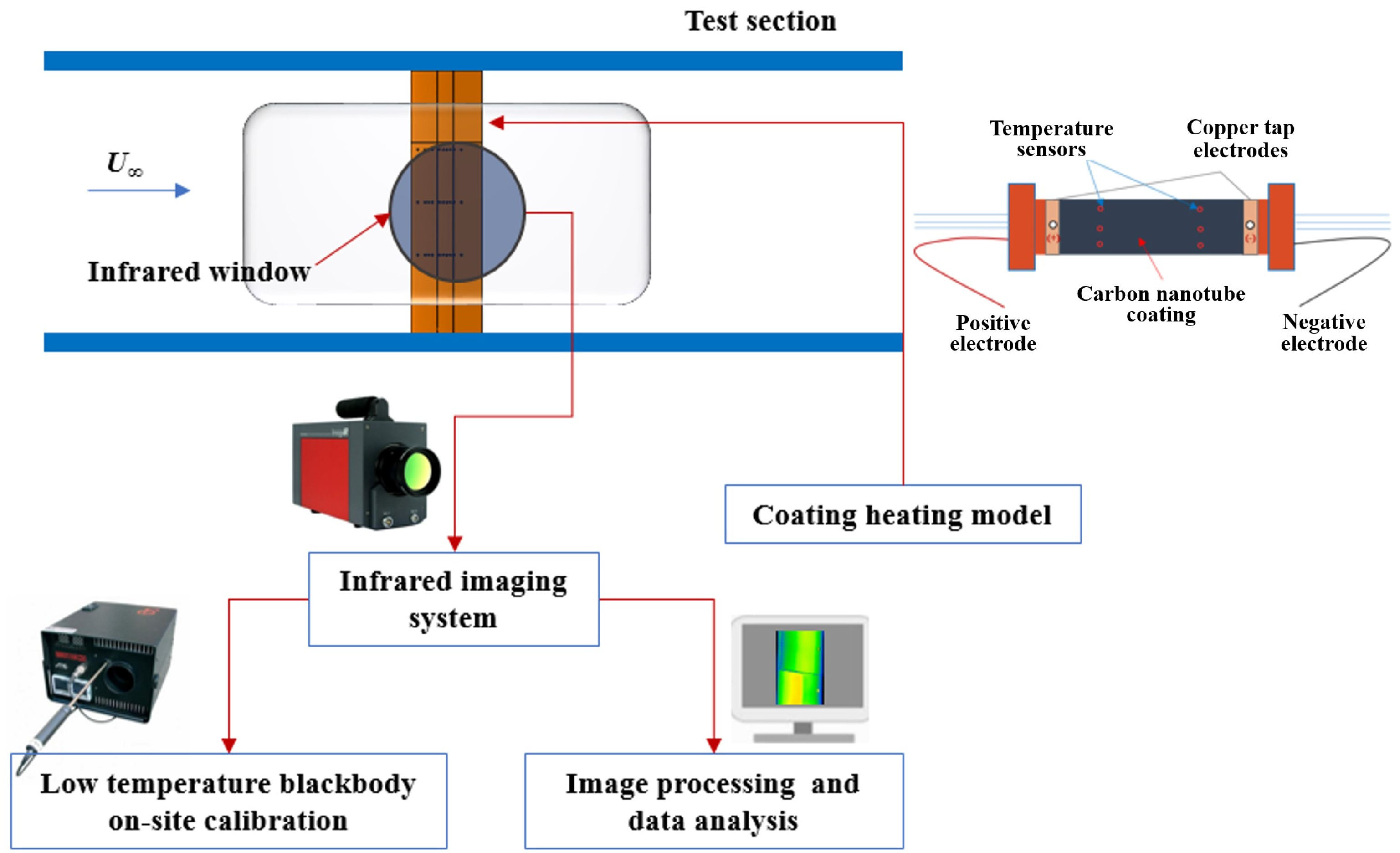
The final model is covered with a heating coating. This coating consists of the upper, the middle, and the lower layers (see Figure 3). The upper and the lower layers are insulation layers. Polyurethane insulating paint is adopted, which has good electrical insulation and heat insulation performance. The thermal conductivity is only 0.018–0.024 W/(m·K), and the softening temperature is high, at 250 °C. The middle layer is a carbon-nanotube conductive water-based coating, which has the advantages of strong adhesion, excellent heating performance, good elasticity and heat aging resistance. Firstly, the lower insulating layer was sprayed onto the surface of the base model and had been naturally solidified for 1 h. Then the carbon-nanotube coating was sprayed onto the lower insulation layer, and had been dried and solidified for 30 min at 80 °C. Finally, the upper insulation layer was sprayed onto the carbon-nanotube coating and had been naturally solidified for 1 h, too. Once the coating was ready, its outer surface would be polished. The thickness d of the whole coating is about 60 μm, with surface roughness of 1.0 μm. The roughness is a little larger than that of the base model.
A pair of copper tape electrodes were arranged at the two ends of the model to connect the heating coating with the power supply. The heating power was adjusted by a control system automatically. According to the temperature measured by the sensors on the model, a feedback control strategy was adopted to achieve the preset temperature. The surface temperature of the model can be adjusted from room temperature to about 50 °C.
2.2. Infrared Measurement System
The infrared measurement system mainly consists of a medium-wave infrared thermal imager (ImageIR 9500, InfraTec, Dresden, Germany, see Figure 4), an infrared lens with a focal length of 25 mm, a set of image acquisition and processing software packages, and a low-temperature blackbody. The thermal imager uses a mercury cadmium telluride (MCT) detector with a maximum resolution of 1280 × 720 pixels, full frame rate of 120 Hz, and measuring range of −20–1500 °C. The R982A low-temperature blackbody provides a temperature source ranging from −20 °C to 150 °C and has very good temperature uniformity. The infrared measurement system has advantages of high resolution, high frame rate, and wide temperature range.
A support platform for the infrared thermal imager was installed outside the observation window (see Figure 4). The platform could realize a position adjustment in three degrees of freedom (the horizontal direction X, the vertical direction Y, and the direction Z). The observation window was also changed to a Si glass, which is fit for medium-wave infrared light. The Si glass has a thickness of 8 mm and a diameter of Φ = 150 mm. The two sides of the Si glass are coated with antireflective films. As a result, the transmittance of medium-wave infrared (3–5 μm) is greater than 90%.
2.3. Wind Tunnel
The test was conducted in the 0.6 m × 0.6 m wind tunnel of the China Aerodynamics Research and Development Center. The wind tunnel is an intermittent subsonic, transonic and supersonic wind tunnel with a cross-section size of 0.6 m × 0.6 m. The test section is 1.775 m long. In the test, the side walls of the test section were solid, with an expansion angle of 0.4°, and the top and bottom walls of the test section were slotted walls. The slotting rate was 4.24%. Figure 5 shows the installation of the model in the wind tunnel.
2.4. Work Frame
Figure 6 shows the work frame of the wind tunnel test. Before the test, the infrared thermal imager was calibrated on-site with the low-temperature blackbody. Electrical heating was carried out until the temperature of the model’s surface reached the preset temperature. Then, starting the wind tunnel, with continuous heating or no heating, infrared images were taken at a specified rate. After each run, the captured images were analyzed with the processing software.
3. Preparation
3.1. Calibration of the Infrared Thermal Imager
Before the wind tunnel test, the infrared thermal imager was calibrated. The low-temperature blackbody was placed at the center of the temperature measurement area. The infrared thermal imager was focused on the blackbody. The temperature of the blackbody was changed from −5 °C to 30 °C with an interval of 5 °C, and the temperatures detected by the infrared thermal imager were recorded. The calibration process was conducted with and without the Si glass (no window) separately. Results are presented in Figure 7. It is seen that the Si glass has a very slight absorption of the infrared light. The least square method was used to fit the temperature data recorded with the Si glass. A correction formula for temperature was obtained. This formula was used in the wind tunnel test.
3.2. Heating Uniformity
Another task that needed to be performed before the wind tunnel test was the analysis of heating uniformity. The test model’s temperature was set as 30 °C. After the heating power was stable, the temperature of the suction side of the model was measured by infrared thermography, as well as by the six temperature sensors. Figure 8 shows the temperature distributions along three chordwise lines, which are at the 45%, 52% and 58% span sections. The temperature distribution along each line is relatively uniform with a difference of less than 1 °C, except for the first 2% chord length (near the leading edge) and the last 3% chord length (near the trailing edge). In general, the heating uniformity is very good. It should be noted that the temperature along the line at the 45% span section is about 1 °C lower than the temperatures along the other two lines. Because only the measurement of the No. 1 temperature sensor was used as the feedback in the temperature control process, the temperatures along the three lines were all lower than the set temperature.
Table 1 lists the measurements of the six temperature sensors. The temperatures along the same chordwise line have good uniformity. It is thought that the uniformity has a relationship with the thickness of the heating coating. In the fabrication of the heating coating, the carbon-nanotube coating as well as the insulation paint were sprayed in chordwise direction. Therefore, the heating coating along one chordwise line has almost the same thickness. It can be concluded that the thickness of carbon-nanotube coating affects the heating uniformity. According to the voltage and the resistance of the heating coating, the heating power per unit area was 450 W/m2. The temperature difference on the whole wing surface did not exceed 3 °C.
4. Results and Discussion
4.1. Simulation Method
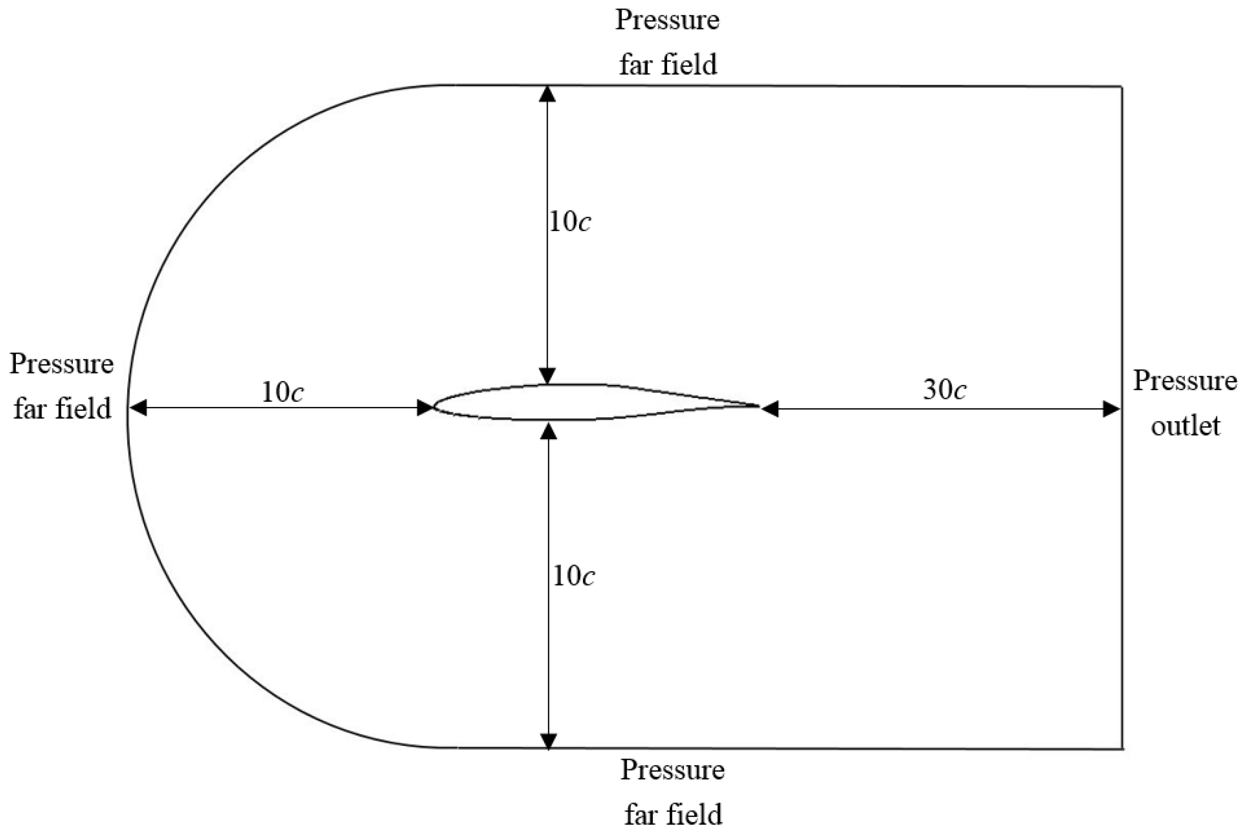
Numerical simulations were also conducted to study the transition characteristics of the modified RAE5243 airfoil. Figure 9 shows the schematic of the calculation domain and the boundary conditions. The airfoil is not drawn to scale in this figure. The surface of the airfoil was set as no slip wall condition. Without heating, the wall was adiabatic, while with heating, a specified heat flux was arranged on the wall. The y+ of the first layer of the grid on the airfoil’s surface was slightly less than 1. The transition model of SST model was adopted to predict the transition of the boundary layer. The turbulence intensity of the incoming flow was set to 1%, and the turbulence viscosity ratio was set to 15.
The SST transition model is the SST turbulence model coupled with transition model [23]. The transport equations for the turbulent kinetic energy k, the turbulent frequency ω, the intermittency γ, and the transition momentum thickness Reynolds number Reθ are listed as follows.
Details of the transport equations are referred to in Refs. [23,24]. Steady simulations were conducted, and a second-order upwind scheme for spatial discretization was utilized. The convective flux was evaluated by the Roe flux-difference splitting scheme. The following expression was used for discrete flux at each face.
Here is the spatial difference QRQL. The fluxes FR = F(QR) and FL = F(QL) are computed using the solution vectors QR and QL on the “right” and “left” side of the face. The matrix is defined by
where is the diagonal matrix of eigenvalues and M is the modal matrix that diagonalizes , where A is the inviscid flux Jacobian .
Firstly, a validation simulation of the original RAE5243 airfoil was carried out. Figure 10 compares the distributions of static pressure over the RAE5243 airfoil obtained from the paper [25] and from the present simulation. It can be seen that the two distributions of static pressure agree well, which means that the present simulation is reliable.
For the modified RAE5243 airfoil, the inflow conditions are listed in Table 2. They are the same as those of the wind tunnel test. At Ma = 0.7, a grid independence verification was carried out. The local grid around the airfoil is shown in Figure 11. The number of grids in Block 1 presented in red color was changed from 328 × 131 to 727 × 131. The results of the lift coefficient CL, the drag coefficient CD, the relative transition location on the upside x*up/c, and the relative transition location on the downside x*down/c are listed in Table 3. It seems that the four results are converged after Grid-3, which has 660 × 131 grids. So Grid-3 was used in this numerical study.
The method of detecting the transition location has been determined. Both the turbulent kinetic energy (TKE) and the temperature on the suction side of the airfoil are extracted from the simulation results. For the TKE, the position where it increases sharply (with the maximum gradient) is regarded as the transition location. For the temperature, there are two situations. Without heating, the temperature of the airfoil surface is lower than the recovery temperature of the incoming flow. The position where the temperature rises rapidly (with the maximum gradient) is taken as the transition location. With heating, the surface temperature is higher than the static temperature of the surrounding flow. The position where the temperature decreases rapidly (with the minimum gradient) is taken as the transition location.
The effect of heating was studied first. Without and with heating, the distributions of static pressure, TKE and temperature on the suction side of the modified RAE5243 airfoil are compared in Figure 12 under the conditions of Ma = 0.7 and α = 0°. The heat fluxes of 245 W/m2 and 450 W/m2 were close to the heat fluxes in the wind tunnel test with different set temperatures. It is seen that the heating has nearly no impact on the static pressure distribution as well as the TKE distribution. The transition location detected by the TKE gradient was almost the same as that detected by the temperature gradient. The detected transition location did not change in general. Similar results were obtained at other Mach numbers. The numerical results for the effects of AOA and Mach number will be discussed and presented together with the test results in the next section.
4.2. Results and Analysis
- a.
- Impact of the heating power
The impact of the heating power on transition location was experimentally investigated. Three tests with no heating (q = 0 W/m2), the set temperature of 20 °C (q = 245 W/m2) and the set temperature of 30 °C (q = 450 W/m2) were carried out separately. The infrared images were taken after the flow field had been stable for 10 s. Figure 13 shows the distributions of temperature of the three tests under the conditions of Ma = 0.75 and α = 0°. The temperatures are extracted along the same chordwise line on the suction side of the wing. It is found that the heating power has no impact on the transition location. This conclusion is consistent with that derived from the numerical simulations.
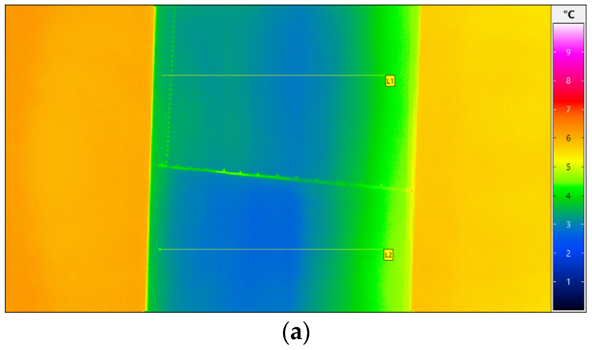
Figure 14 compares the distributions of temperature of the whole suction side without and with heating. The top half of the wing was forced transition with cylindrical elements [26], while the bottom half of the wing was natural transition. Without heating, the natural transition location in the bottom half was hardly detected. The temperature of the turbulent flow region that is just behind the transition strip in the top half is close to the temperature of the laminar flow region that is at the same streamwise location in the bottom half. However, with heating, the natural transition location in the bottom half is visible, and the temperature difference between the turbulent flow region and the laminar flow region at the same streamwise location is apparent. It proves that the technique combining infrared thermography and carbon-nanotube coating is effective.
- b.
- Effect of AOA
With the set temperature of 30 °C (q = 450 W/m2), the transition locations of the boundary layer on the suction side were detected at different AOA. Figure 15 shows the distributions of temperature on the suction side under the conditions of Ma = 0.75 and α = −3°, 0° and 3°. The transition locations detected by the temperature gradient are also marked in the figure. Figure 16 compares the trends of transition location with the increase in AOA obtained from the wind tunnel test and the numerical simulations. The two trends are consistent. As the AOA increases, the transition location moves forward. When the model is at negative AOA, the stagnation point moves to the suction side, which enhances the downstream favorable pressure gradient. Therefore, the transition caused by adverse pressure gradient is delayed, and the transition location moves downstream. When the model is at positive AOA, the stagnation point moves to the pressure side. The airflow around the leading edge of the wing expands rapidly, leading to the exacerbation of adverse pressure gradient on the suction side. This makes the transition location move forward. At high Mach numbers and positive AOA, a shock wave appears on the suction side (see Figure 17). The shock wave induces separation of the boundary layer, thus promoting the transition of the boundary layer. In that condition, the transition location is closely related to the shock wave.
- c.
- Effect of Mach number
Figure 18 shows the distributions of temperature on the suction side with different Mach numbers at α = 0°. The transition locations detected by the temperature gradient are also marked in the figure. It is seen that the trend of the transition location with Mach number is not monotonic. As Mach number increases from 0.4 to 0.75, the transition location moves forward from 55.7% to 50.3%. As Mach number increases from 0.75 to 0.9, the transition location moves backward from 50.3% to 57.7%. Figure 19 compares the trends of the transition location with Mach number obtained from the wind tunnel test and the numerical simulations. It seems that the two trends are consistent.
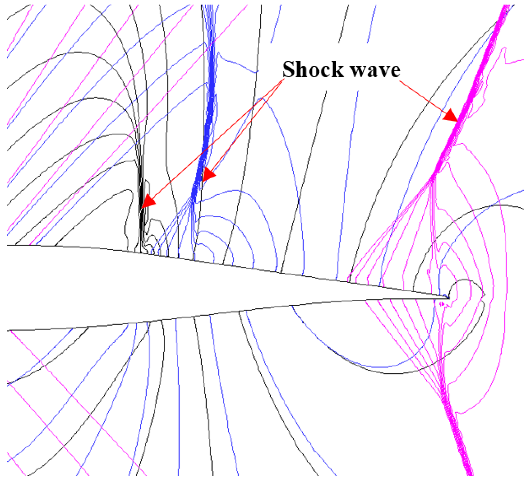
Figure 20 shows that a shock wave appears on the suction side of the wing at Ma = 0.75, while it does not appear at Ma = 0.7. The appearance of the shock wave changes the mechanism of transition. In the condition of Ma < 0.75, transition is closely related to adverse pressure gradient. The adverse pressure gradient promotes the rapid growth of T-S instability in the boundary layer, thus inducing the transition. As the Mach number increases, the lowest point of static pressure moves forward, exacerbating the downstream adverse pressure gradient. Therefore, the transition location moves forward. In the condition of Ma 0.75, a shock wave appears and induces separation of the boundary layer. The K-H instability in the shear layer of the separation promotes the transition. Therefore, the transition location is closely related to the shock wave’s position. With the increase in Mach number, the shock wave’s position moves backward (see Figure 21). As a result, the transition location moves backward.
5. Conclusions
The transition characteristics of a modified RAE5243 airfoil were investigated by a wind tunnel test and numerical simulations. A technique combining infrared thermography and carbon-nanotube coating was utilized to detect the transition location. With this technique, the accuracy of transition location was improved significantly.
Firstly, the heating uniformity of the carbon-nanotube coating was checked. It was found that the heating uniformity was affected by the thickness of the carbon-nanotube coating. The test as well as the simulations validated that heating power had no impact on the transition location.
The effects of AOA and Mach number on the transition location were studied. As the AOA increases, the transition location on the suction side of the modified RAE5243 airfoil moves forward. With an increase in Mach number, the transition location moves forward first and then backward. It reaches its most forward point at Ma = 0.75. This change is attributed to the appearance of a shock wave. In the range of Ma = 0.75~0.90, the shock wave appears on the suction side, and the transition location is closely related to the shock wave’s position rather than the adverse pressure gradient.
Author Contributions
Conceptualization, Z.L. and H.W.; methodology, Z.L., H.W. and F.Q.; validation, Z.Z. and X.L.; formal analysis, Z.L. and H.W.; investigation, Z.L. and H.W.; writing—original draft preparation, Z.L.; writing—review and editing, Z.L. and H.W. All authors have read and agreed to the published version of the manuscript.
Funding
This research received no external funding.
Data Availability Statement
The data presented in this study are available on request from the corresponding author due to privacy.
Conflicts of Interest
The authors declare no conflicts of interest.
References
- Schrauf, G. Status and perspectives of laminar flow. Aeronaut. J. 2005, 109, 639–644. [Google Scholar] [CrossRef]
- Thibert, J.J.; Reneaux, J.; Schmitt, R.V. ONERA Activities on Drag Reduction. ICAS-90-3.6.1. 1990. Available online: https://www.icas.org/ICAS_ARCHIVE/ICAS1990/ICAS-90-3.6.1.pdf (accessed on 21 February 2023).
- Lai, G.J.; Li, Z.D.; Zhang, Y.Z. Research on natural laminar airfoil wind tunnel test at high Reynolds number. Aeronaut. Sci. Technol. 2017, 28, 12–15. [Google Scholar]
- Streit, T.; Horstmann, K.H.; Schrauf, G.; Hein, S.; Fey, Y.; Egami, A.; Perraud, J.; El Din, I.S.; Cella, U.; Quest, J. Complementary numerical and experimental data analysis of the ETW TELFONA Pathfinder wing transition tests. In Proceedings of the 49th AIAA Aerospace Sciences Meeting including the New Horizons Forum and Aerospace Exposition, Orlando, FL, USA, 4–7 January 2011. [Google Scholar]
- Vermeersch, O.; Yoshida, K.; Ueda, Y.; Arnal, D. Natural laminar flow wing for supersonic conditions: Wind tunnel experiments, flight test and stability computations. Prog. Aerosp. Sci. 2015, 79, 64–91. [Google Scholar] [CrossRef]
- Collifer, F.S. An Overview of Recent Subsonic Laminar Flow Control Flight Experiments. AIAA-1993-2987. 1993. Available online: https://arc.aiaa.org/doi/10.2514/6.1993-2987 (accessed on 23 February 2023).
- Zhu, Z.Q.; Wu, Z.C.; Chen, Y.C.; Vicente, J.; Valero, E. Advanced Technology of Aerodynamic Design for Commercial Aircraft; Shanghai Jiaotong University Press: Shanghai, China, 2013. [Google Scholar]
- Fujino, M.; Yoshizaki, Y.; Kawamura, Y. Natural-laminar-flow airfoil development for a lightweight business jet. J. Aircr. 2003, 40, 609–615. [Google Scholar] [CrossRef]
- Fujino, M. Design and development of the Honda jet. J. Aircr. 2005, 42, 755–764. [Google Scholar] [CrossRef]
- Hiroaki, I.; Yoshine, U.; Naoko, T. Natural laminar flow wing design for a low-boom supersonic aircraft. In Proceedings of the AIAA SciTech Forum, Grapevine, TX, USA, 9–13 January 2017. [Google Scholar]
- Owens, L.R.; Beeler, G.B.; King, R.A.; Chou, A.; Balakumar, P.; Banks, D. Supersonic traveling crossflow wave characteristics in ground and flight tests. In Proceedings of the AIAA SciTech Forum, Orlando, FL, USA, 6–10 January 2020. [Google Scholar]
- Wang, F.; Eriqitai, W.Q.; Schulein, E. Experimental investigation of HLFC mechanism on swept wing. J. Aerosp. Power 2010, 25, 918–924. [Google Scholar]
- Sugiura, H.; Yoshida, K.; Tokugawa, N.; Takagi, S.; Nishizawa, A. Transition measurements on the natural laminar flow wing at Mach 2. J. Aircr. 2002, 39, 996–1002. [Google Scholar] [CrossRef]
- Costantini, M.; Henne, U.; Risius, S.; Klein, C. A robust method for reliable transition detection in temperature-sensitive paint data. Aerosp. Sci. Technol. 2021, 113, 106702. [Google Scholar] [CrossRef]
- Fujisawa, N.; Aoyama, A.; Kosaka, S. Measurement of shear-stress distribution over a surface by liquid-crystal coating. Meas. Sci. Technol. 2003, 14, 1655–1661. [Google Scholar] [CrossRef]
- Arshia, T.; Massoud, T.; Mehran, M.; Hamidreza, E.; Mehdi, S. An experimental study on boundary layer transition detection over a pitching supercritical airfoil using hot-film sensors. Int. J. Heat. Fluid. Flow. 2020, 86, 108743. [Google Scholar]
- Driver, D.M.; Drake, A. Skin friction measurements using oil film interferometry in the 11’ transonic wind tunnel. AIAA J. 2008, 46, 2401–2407. [Google Scholar] [CrossRef]
- Vavra, A.J.; Solomon, W.D., Jr.; Drake, A. Comparison of boundary layer transition measurement techniques on a laminar flow wing. In Proceedings of the 43rd AIAA Aerospace Sciences Meeting and Exhibit, Reno, NV, USA, 10–13 January 2005. [Google Scholar]
- Garbeff, T.J., II; Baerny, J.K. Recent advancements in the infrared flow visualization system for the NASA Ames unitary plan wind tunnels. In Proceedings of the AIAA SciTech Form, Grapevine, TX, USA, 9–13 January 2017. [Google Scholar]
- Geng, Z.H.; He, X.Z.; Wang, X.N.; Yang, Z. Non-intrusive test technique investigation of transition measurement with infrared image in low speed wind tunnel. J. Exp. Fluid. Mech. 2010, 24, 77–82. [Google Scholar]
- Klein, C.; Henne, U.; Yorita, D.; Ondruss, V.; Beifuss, O.; Hensch, A.-K.; Quest, J. Application of carbon nanotubes and temperature-sensitive paint for the detection of boundary layer transition under cryogenic conditions. In Proceedings of the AIAA SciTech Form, Grapevine, TX, USA, 9–13 January 2017. [Google Scholar]
- Goodman, K.Z.; Lipford, W.E.; Watkins, A.N. Boundary-layer detection at cryogenic conditions using temperature sensitive paint coupled with a carbon nanotube heating layer. Sensors 2016, 16, 2062. [Google Scholar] [CrossRef] [PubMed]
- Langtry, R.B.; Menter, F.R. Correlation-based transition modeling for unstructured parallelized computational fluid dynamics codes. AIAA J. 2009, 47, 2894–2906. [Google Scholar] [CrossRef]
- Menter, F.R. Two-Equation Eddy-Viscosity Turbulence Models for Engineering Applications. AIAA J. 1994, 32, 1598–1605. [Google Scholar] [CrossRef]
- Fulker, J.L.; Simmons, M.J. An experimental investigation of passive shock/boundary-layer control on an aerofoil. In EUROSHOCK-Drag Reduction by Passive Shock Control; Notes on Numerical Fluid Mechanics; Stanewsky, E., Delery, J., Fulker, J., Geissler, W., Eds.; Friedr. Vieweg and Sohn Verlagsgesellschaft mbH: Braunschweig/Wiesbaden, Germany, 1997. [Google Scholar]
- Huang, Y.; Qian, F.X.; Yu, K.L.; He, B.H.; Chang, L.X.; Lin, X.D. Experimental investigation on boundary-layer artificial transition based on transition trip disk. J. Exp. Fluid. Mech. 2006, 20, 59–62. [Google Scholar]
Figure 1.
Shape of the test model.

Figure 2.
Profiles of the modified RAE5243 airfoil and the original airfoil.
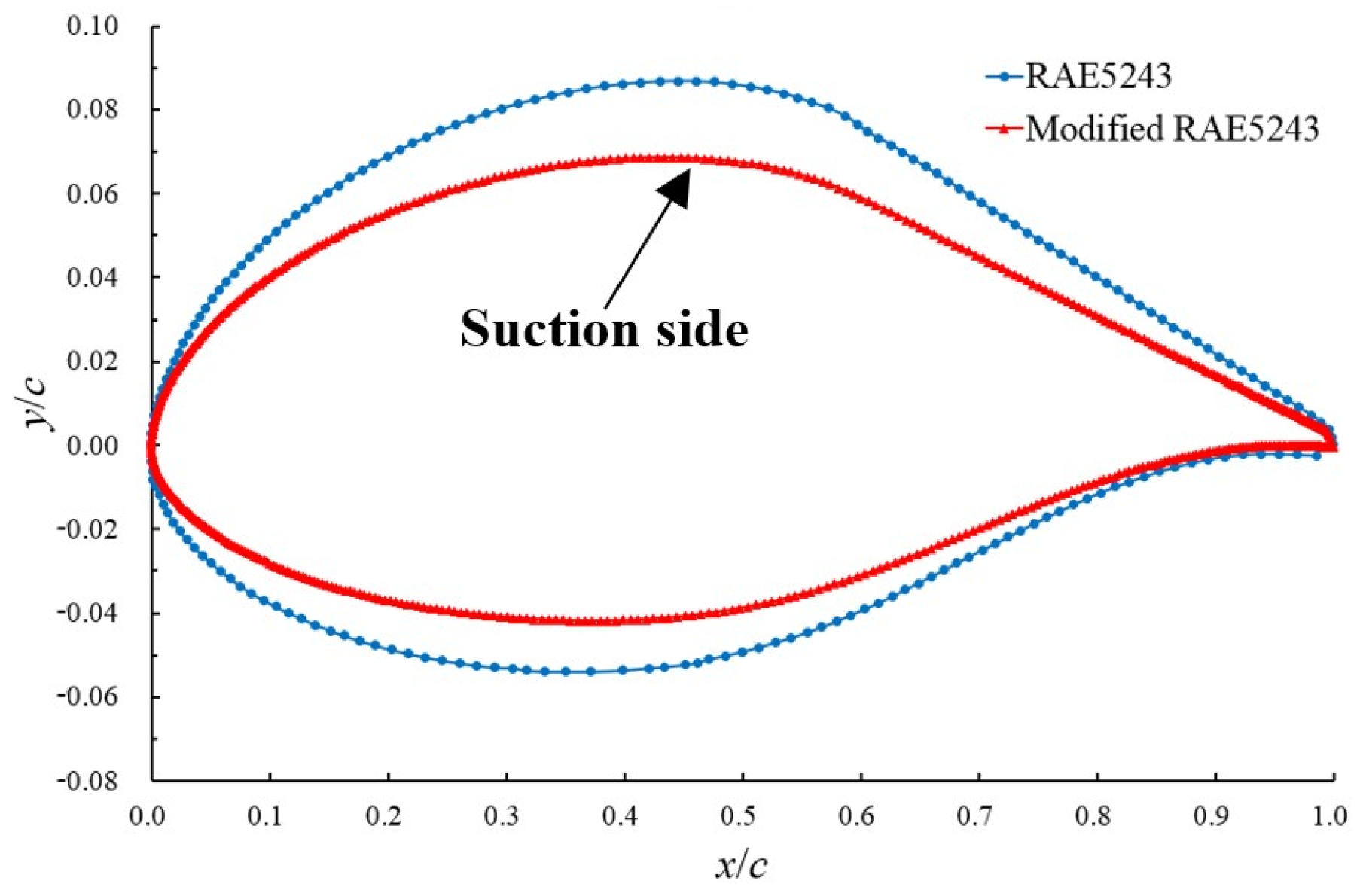
Figure 3.
Schematic of the heating coating.
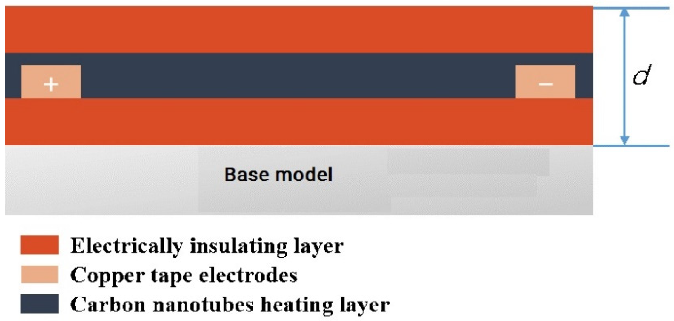
Figure 4.
The IR thermal imager.
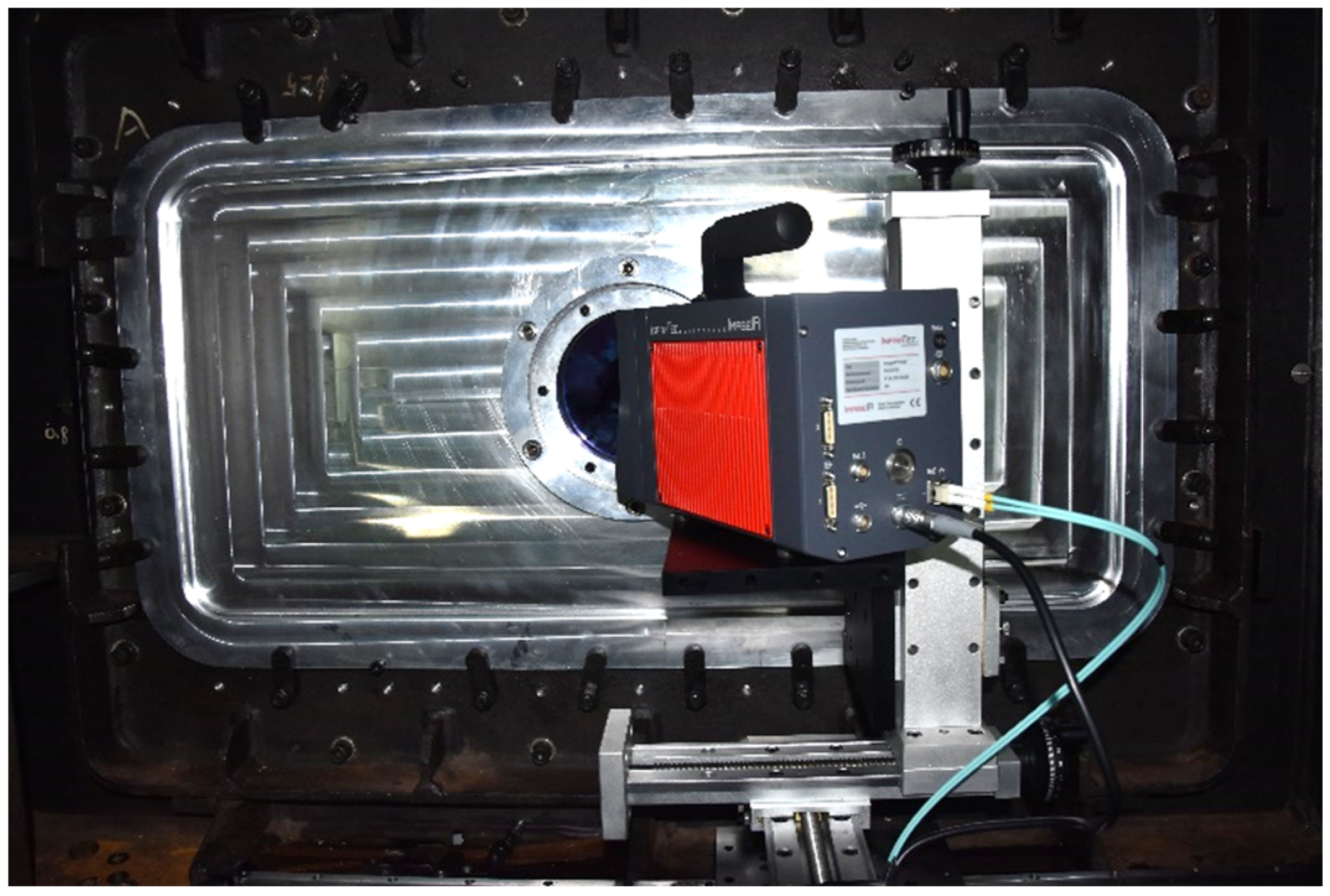
Figure 5.
The model installed in the wind tunnel.
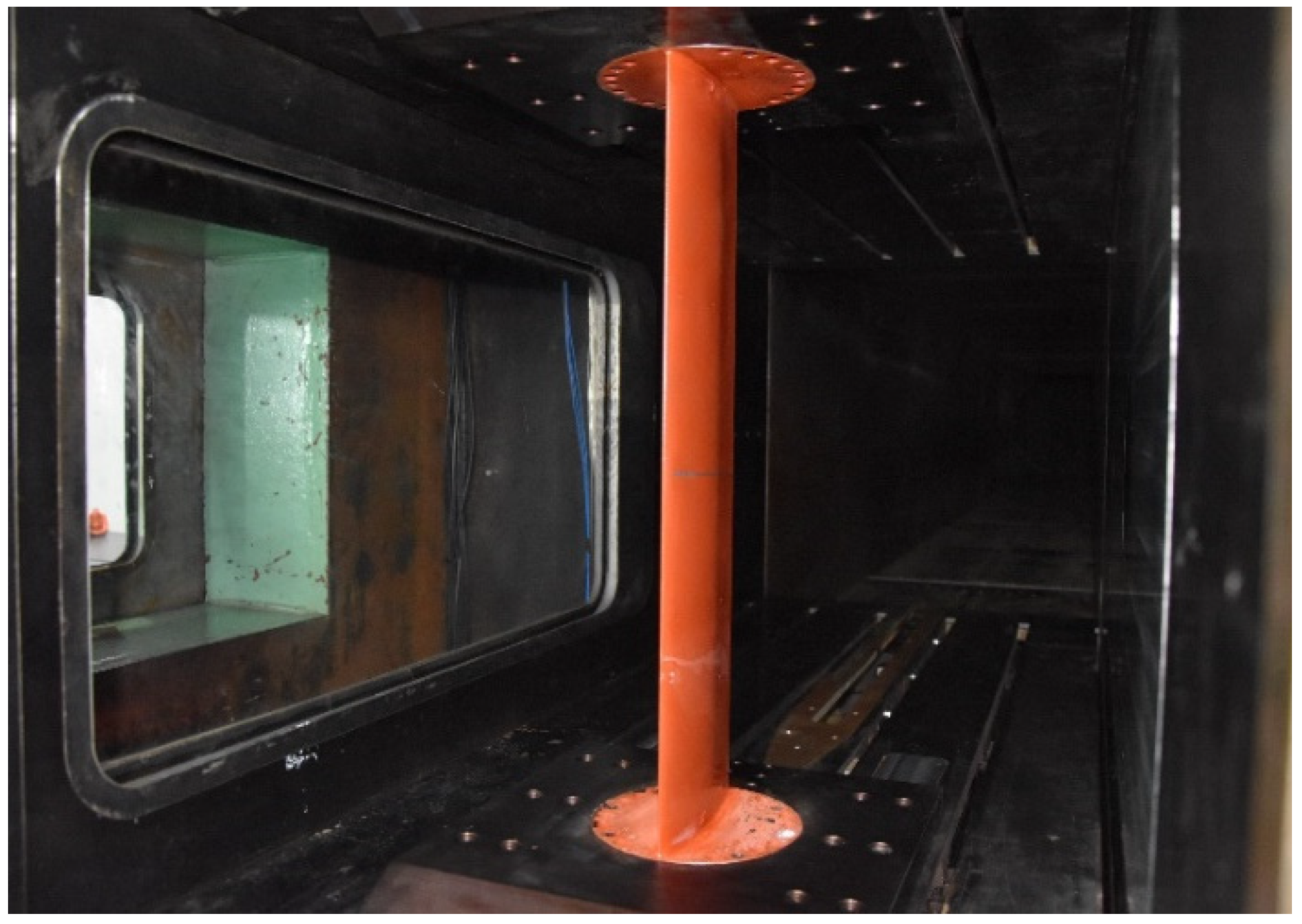
Figure 6.
Work frame of the test.

Figure 7.
Calibration curve of the infrared thermal imager.
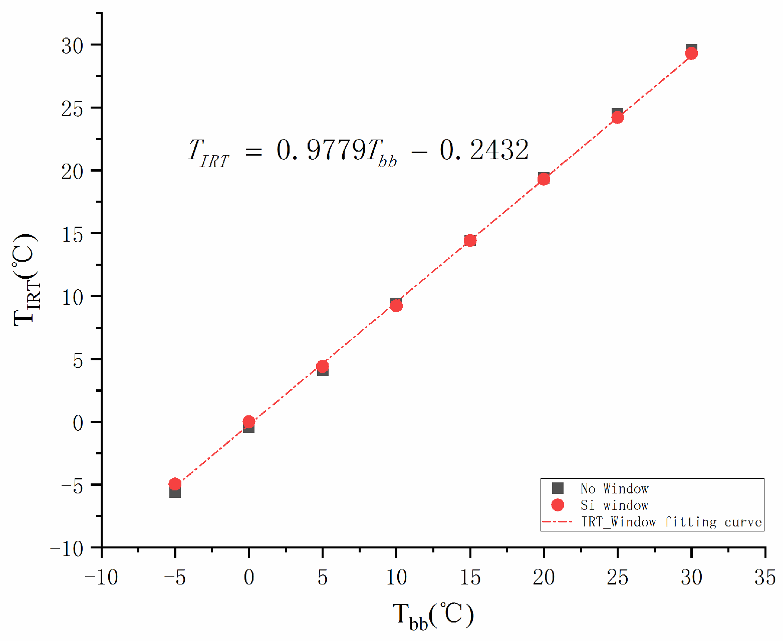
Figure 8.
The heating uniformity.
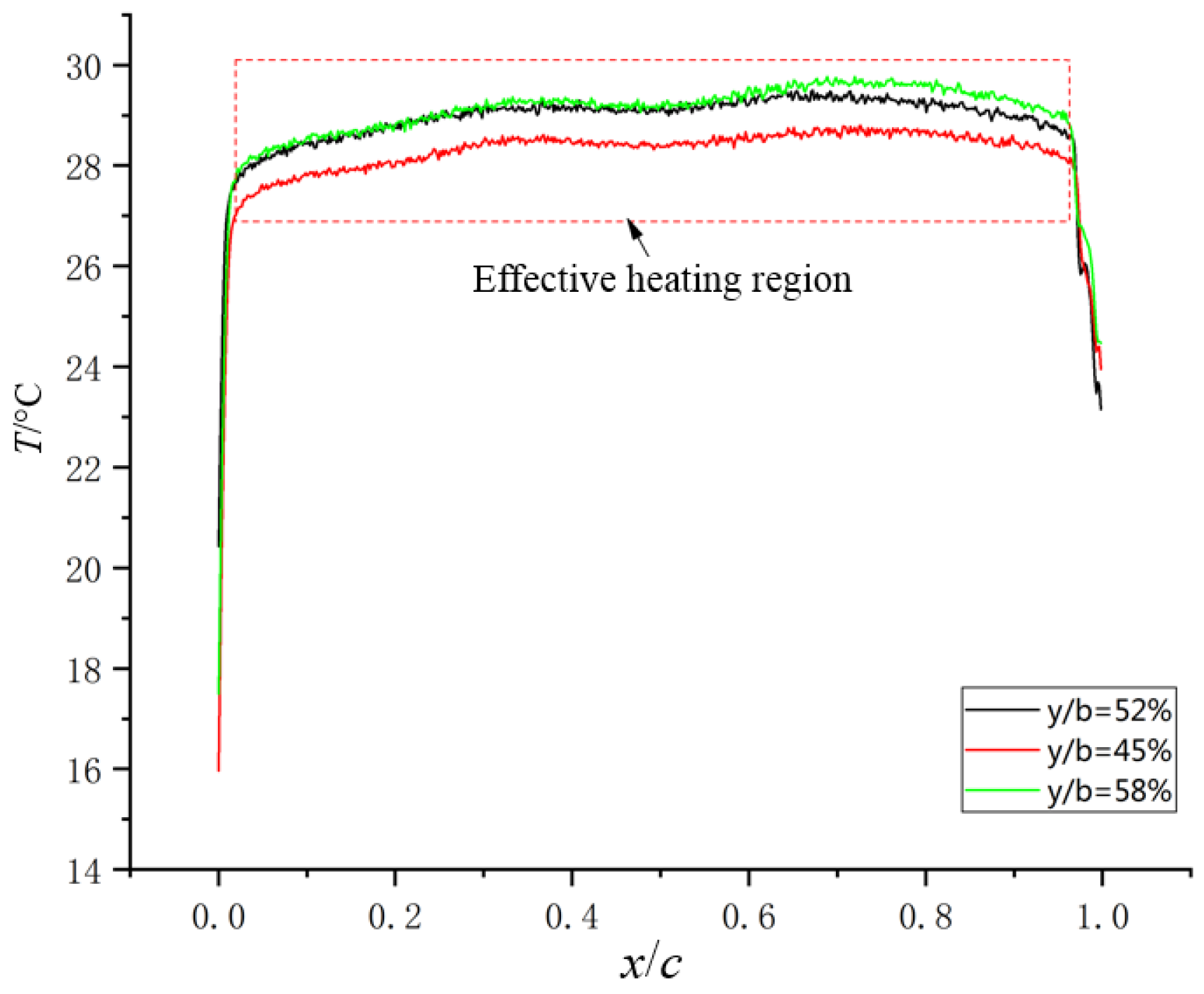
Figure 9.
The calculation domain and the boundary conditions.

Figure 10.
Comparison of static pressure distributions over RAE5243 airfoil.
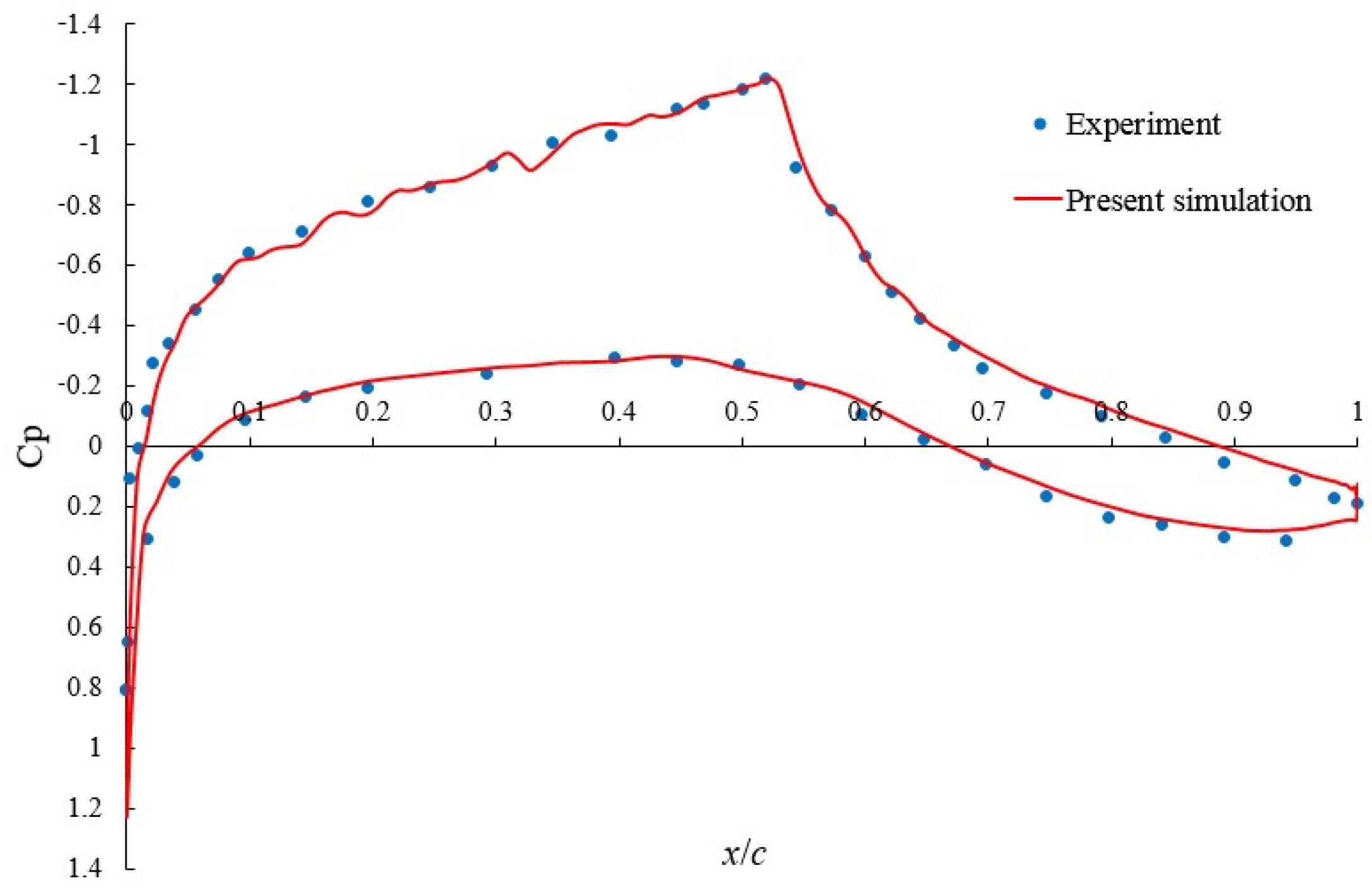
Figure 11.
Schematic of the local grid around the airfoil.
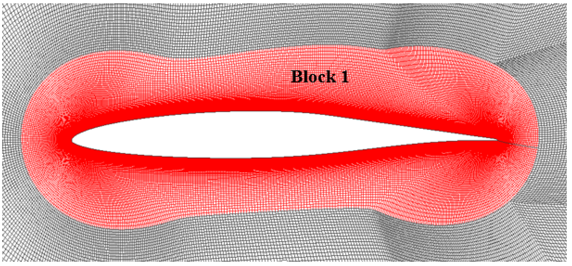
Figure 12.
Comparison of the results without and with heating. (a) Static pressure; (b) TKE; (c) temperature.
Figure 12.
Comparison of the results without and with heating. (a) Static pressure; (b) TKE; (c) temperature.
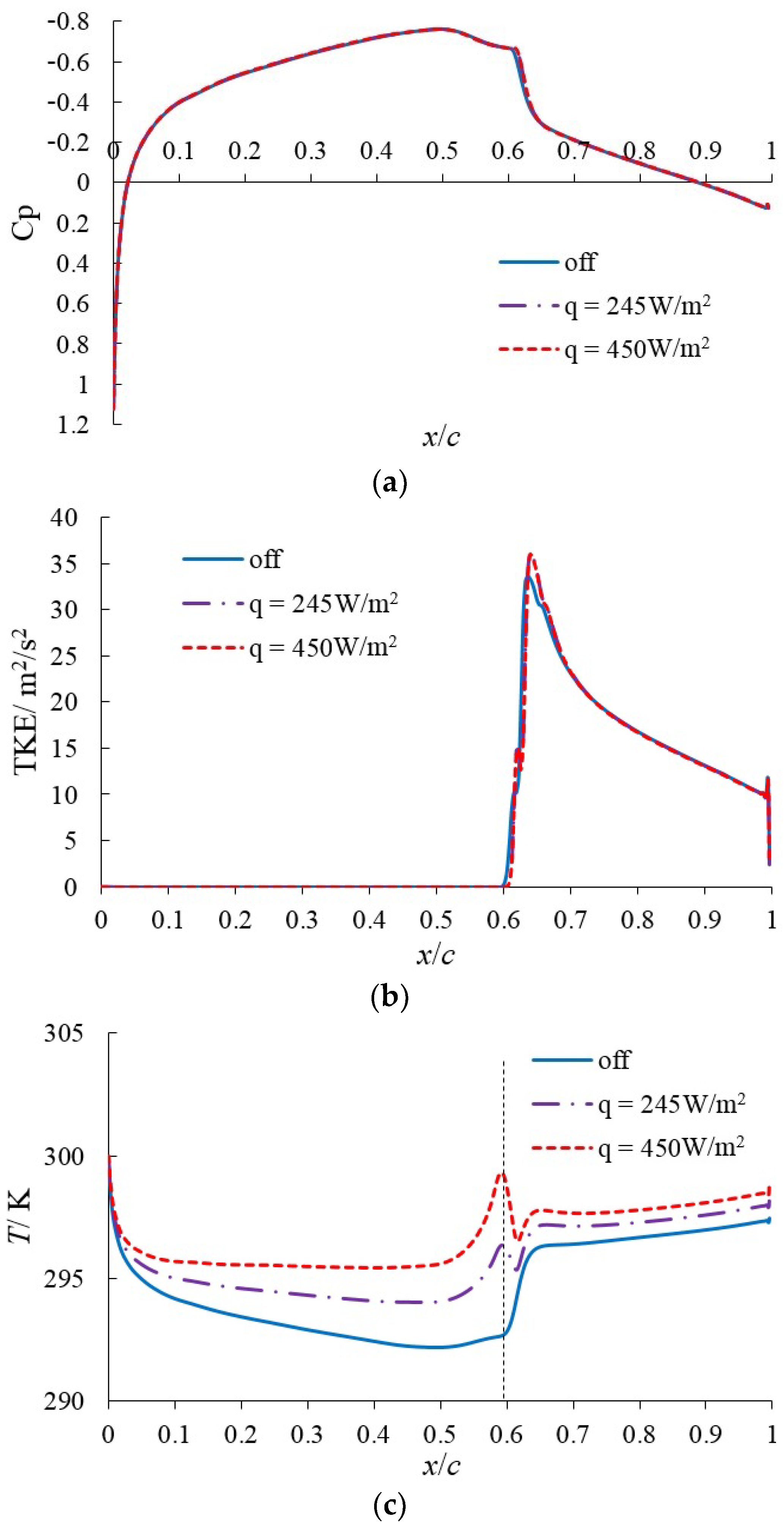
Figure 13.
Effect of heating power on transition location.
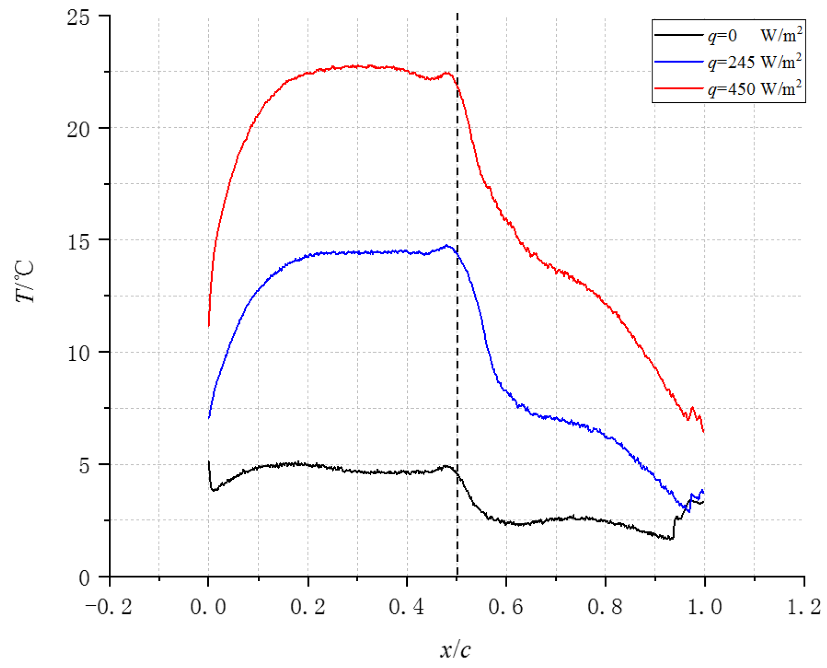
Figure 14.
Comparison of distributions of temperature without and with heating. (a) Without heating; (b) with heating.
Figure 14.
Comparison of distributions of temperature without and with heating. (a) Without heating; (b) with heating.


Figure 15.
Effect of AOA on transition location.
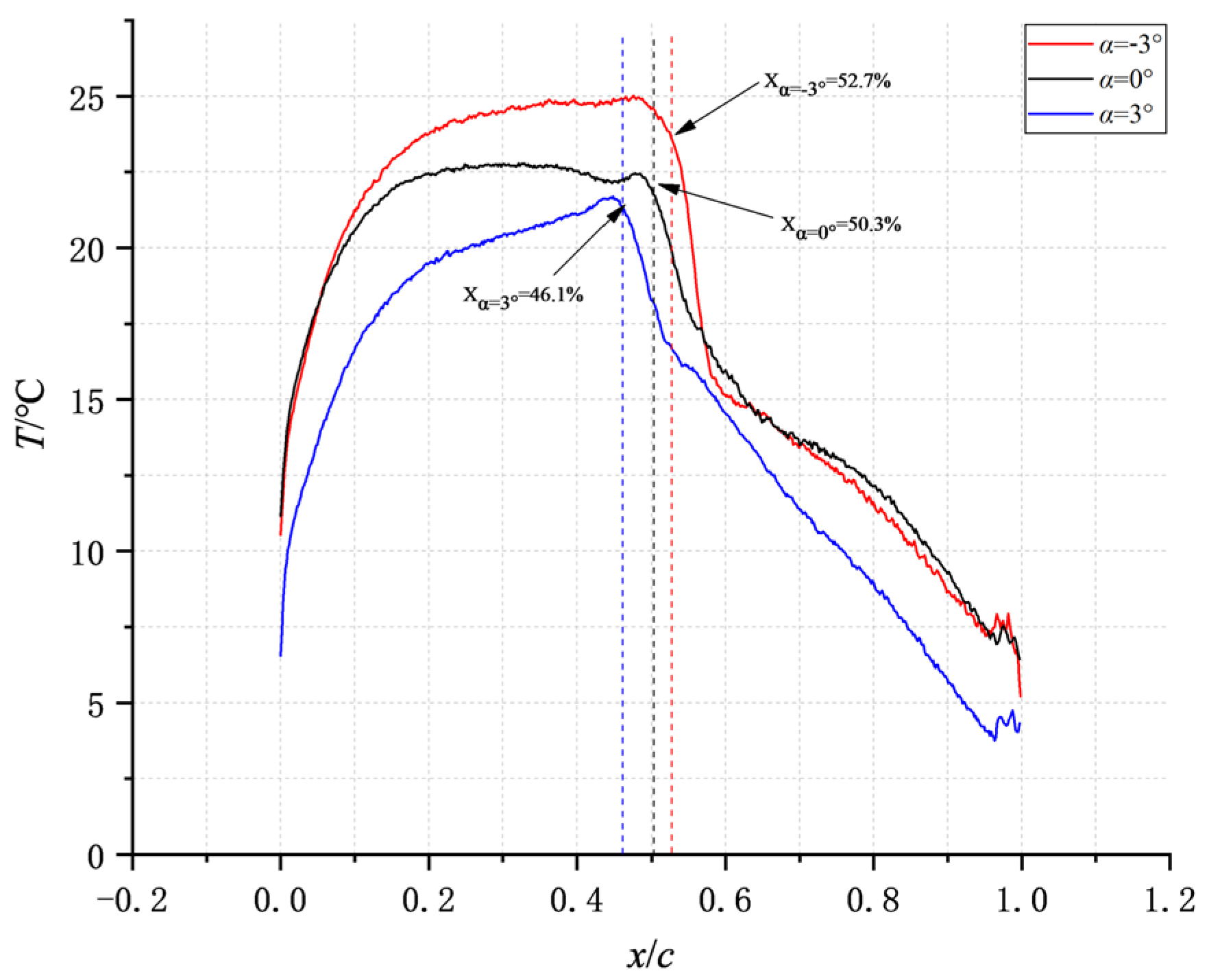
Figure 16.
Comparison of the trends of transition location with AOA (Ma = 0.75).
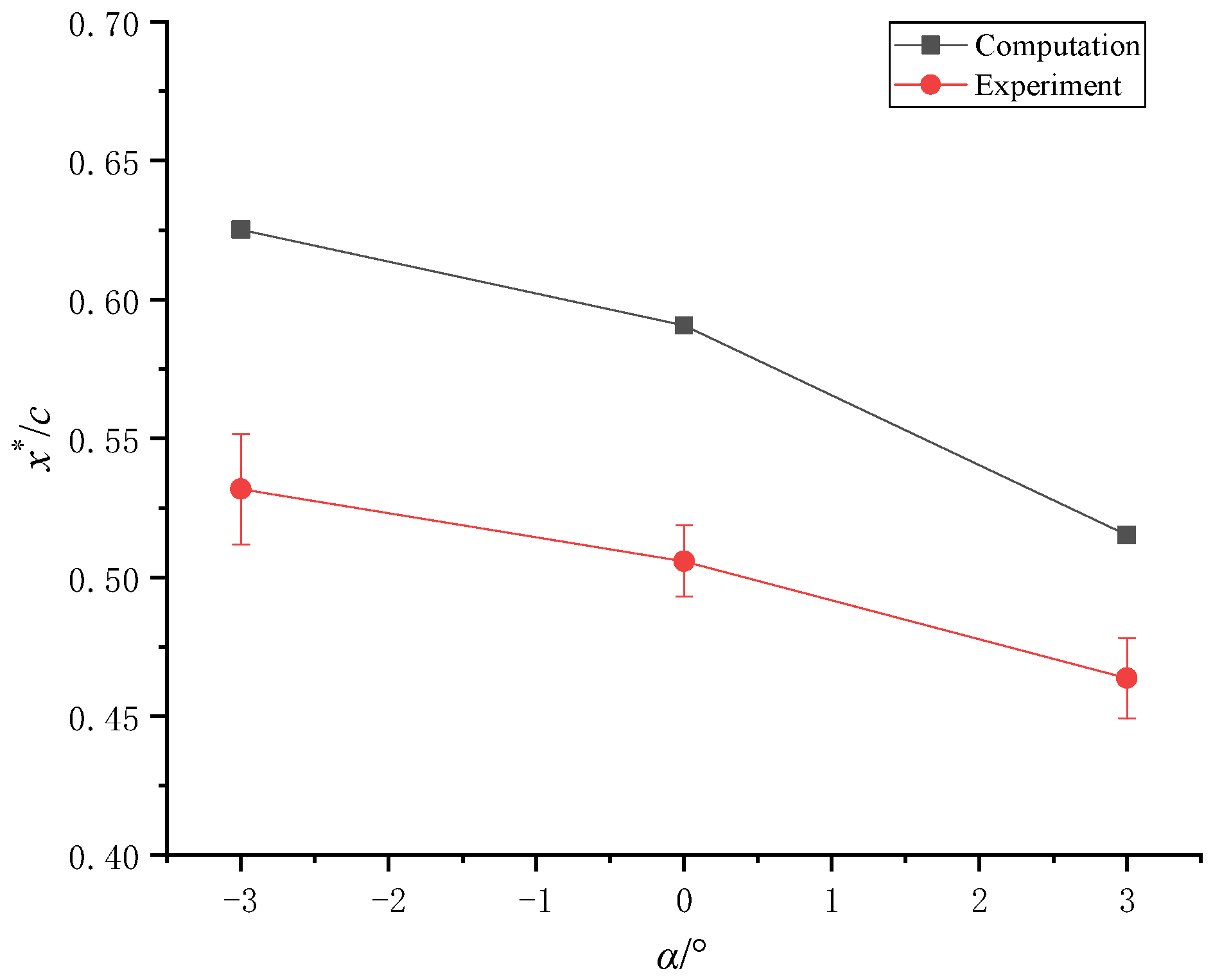
Figure 17.
Iso-line of Ma = 1 at Ma = 0.7 and α = 3°.
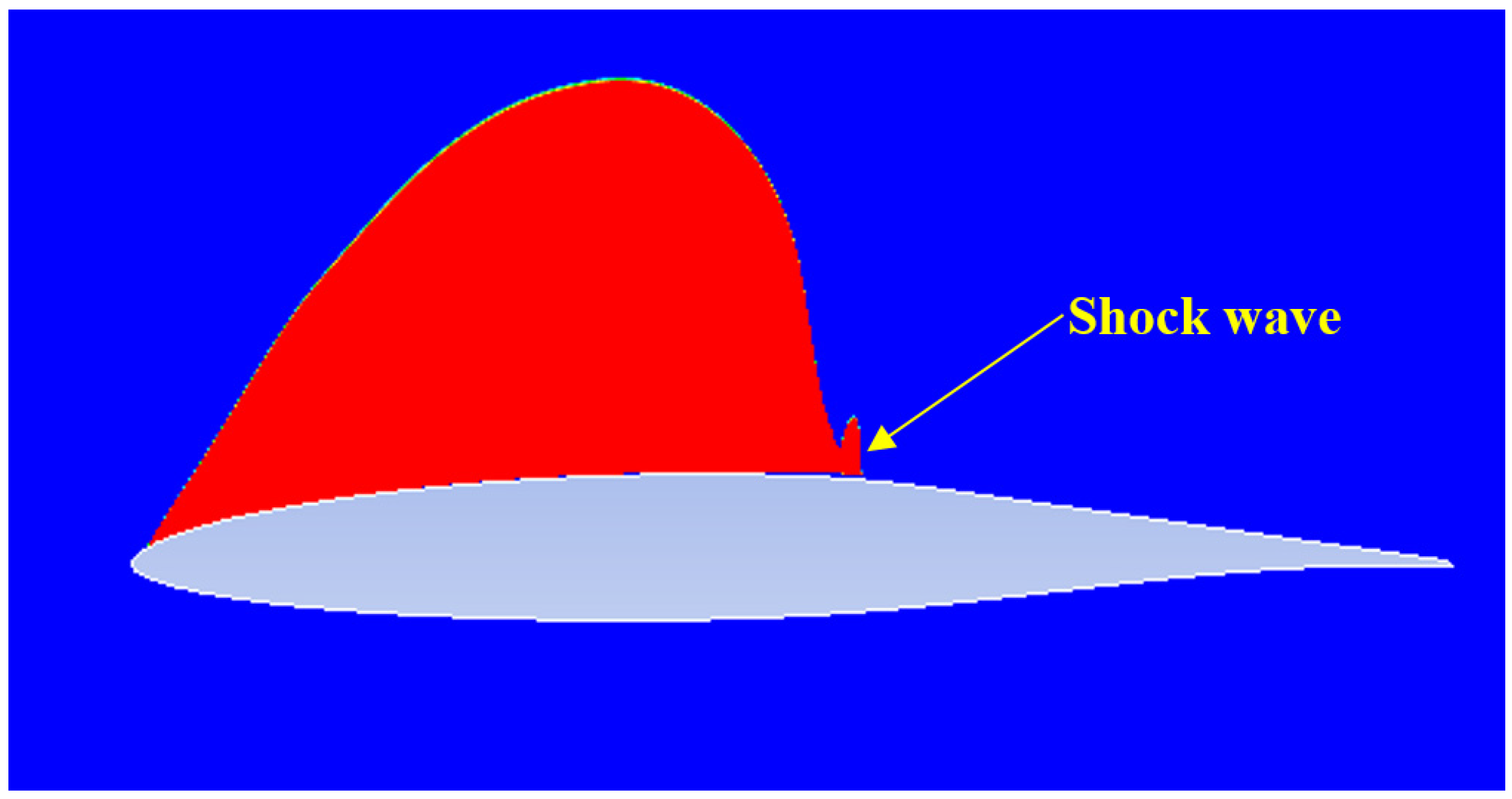
Figure 18.
Effect of Mach number on transition location (α = 0°).
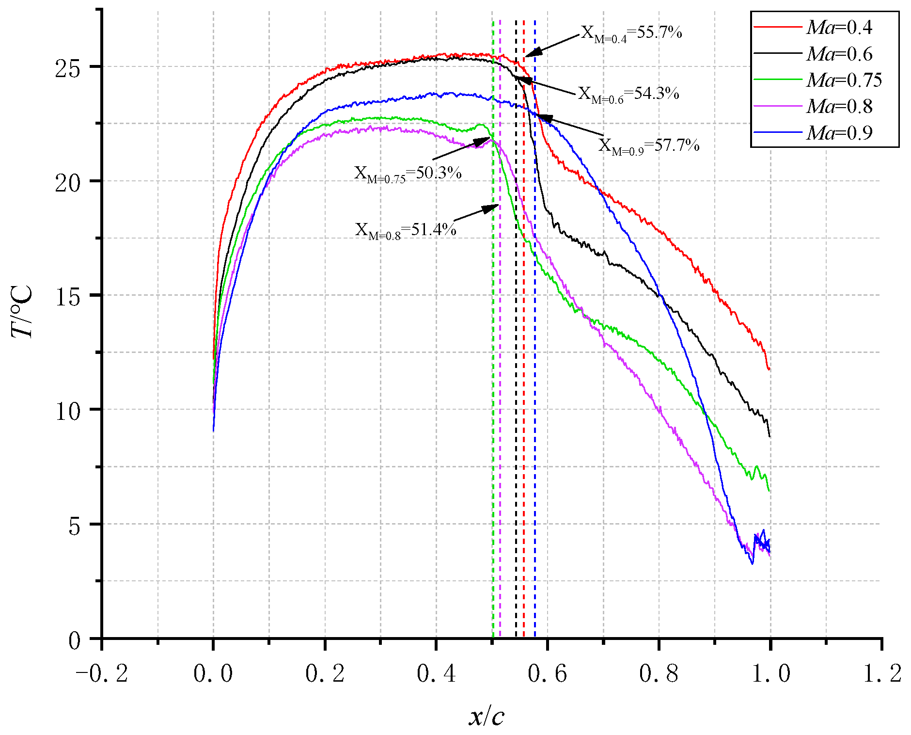
Figure 19.
Comparison of the trends of transition location with Mach number (α = 0°).
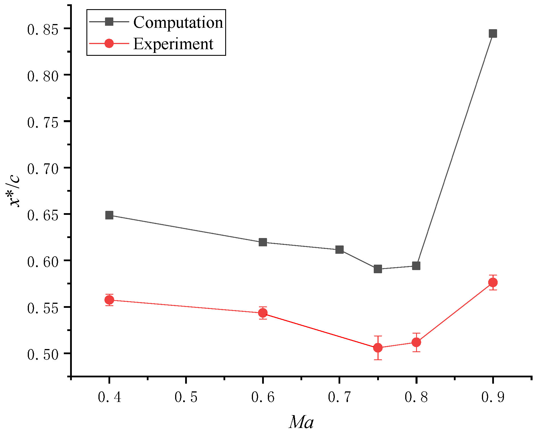
Figure 20.
Iso-line of Ma = 1 at different Mach numbers and α = 0°. (a) Ma = 0.7; (b) Ma = 0.75.

Figure 21.
Shock wave’s positions at different Mach numbers and α = 0° (static pressure lines: black, Ma = 0.75; blue, Ma = 0.8; pink, Ma = 0.9).
Figure 21.
Shock wave’s positions at different Mach numbers and α = 0° (static pressure lines: black, Ma = 0.75; blue, Ma = 0.8; pink, Ma = 0.9).

Table 1.
Measurements of the six temperature sensors.
| 30% Span Section | 70% Span Section | |||||
|---|---|---|---|---|---|---|
| No. | 1 | 2 | 3 | 4 | 5 | 6 |
| T/°C | 30.1 ± 0.2 | 29.3 ± 0.2 | 29.5 ± 0.2 | 28.0 ± 0.2 | 27.0 ± 0.2 | 28.7 ± 0.2 |
Table 2.
The inflow conditions.
| Ma | 0.4 | 06 | 0.7 | 0.75 | 0.8 | 0.9 |
|---|---|---|---|---|---|---|
| P∞/Pa | 89,560 | 79,180 | 75,700 | 72,300 | 72,160 | 67,995 |
| T∞/K | 291 | 280 | 273 | 270 | 266 | 258 |
Table 3.
Results with different grids.
| Block 1 | CL | CD | x*up/c | x*down/c | |
|---|---|---|---|---|---|
| Grid-1 | 328 × 131 | 0.338197 | 0.006702 | 0.614394 | 0.619396 |
| Grid-2 | 494 × 131 | 0.316018 | 0.006556 | 0.630063 | 0.627264 |
| Grid-3 | 660 × 131 | 0.302512 | 0.006454 | 0.627642 | 0.631153 |
| Grid-4 | 727 × 131 | 0.299501 | 0.006433 | 0.629443 | 0.632857 |
Disclaimer/Publisher’s Note: The statements, opinions and data contained in all publications are solely those of the individual author(s) and contributor(s) and not of MDPI and/or the editor(s). MDPI and/or the editor(s) disclaim responsibility for any injury to people or property resulting from any ideas, methods, instructions or products referred to in the content. |
© 2024 by the authors. Licensee MDPI, Basel, Switzerland. This article is an open access article distributed under the terms and conditions of the Creative Commons Attribution (CC BY) license (https://creativecommons.org/licenses/by/4.0/).
Share and Cite
MDPI and ACS Style
Liu, Z.; Wang, H.; Zhang, Z.; Liu, X.; Qian, F. Investigation on Transition Characteristics of a Modified RAE5243 Airfoil. Energies 2024, 17, 1489. https://doi.org/10.3390/en17061489
AMA Style
Liu Z, Wang H, Zhang Z, Liu X, Qian F. Investigation on Transition Characteristics of a Modified RAE5243 Airfoil. Energies. 2024; 17(6):1489. https://doi.org/10.3390/en17061489
Chicago/Turabian StyleLiu, Zhiyong, Hongbiao Wang, Zhao Zhang, Xiang Liu, and Fengxue Qian. 2024. "Investigation on Transition Characteristics of a Modified RAE5243 Airfoil" Energies 17, no. 6: 1489. https://doi.org/10.3390/en17061489
Note that from the first issue of 2016, this journal uses article numbers instead of page numbers. See further details here.