Research on Dynamic Economic Dispatch Optimization Problem Based on Improved Grey Wolf Algorithm

Abstract

The dynamic economic dispatch (DED) problem is a typical complex constrained optimization problem with non-smooth, nonlinear, and nonconvex characteristics, especially considering practical situations such as valve point effects and transmission losses, and its objective is to minimize the total fuel costs and total carbon emissions of generating units during the dispatch cycle while satisfying a series of equality and inequality constraints. For the challenging DED problem, a model of a dynamic economic dispatch problem considering fuel costs is first established, and then an improved grey wolf optimization algorithm (IGWO) is proposed, in which the exploitation and exploration capability of the original grey wolf optimization algorithm (GWO) is enhanced by initializing the population with a chaotic algorithm and introducing a nonlinear convergence factor to improve weights. Furthermore, a simple and effective constraint-handling method is proposed for the infeasible solutions. The performance of the IGWO is tested with eight benchmark functions selected and compared with other commonly used algorithms. Finally, the IGWO is utilized for three different scales of DED cases, and compared with existing methods in the literature. The results show that the proposed IGWO has a faster convergence rate and better global optimization capabilities, and effectively reduces the fuel costs of the units, thus proving the effectiveness of IGWO.

1. Introduction

1.1. Power Dispatch Problem

Over the years, with the rapid development of science and technology and the improvement of people’s living standard, the consumption of energy has been increasing, and especially the large amount of electricity used will inevitably bring a huge burden to the power grid; thus, in order to optimize the scheduling of the power system and the utilization efficiency of electricity, dynamic economic dispatch has become a popular research topic for meeting the actual situation of electricity consumption at home and abroad [1].

The dynamic economic dispatch (DED) problem was first proposed by Bechert and Kwanty in 1971 as an extension of static economic dispatch (SED) [1]. It mainly refers to dividing a day into several periods and optimizing daily economic dispatches based on daily load forecasts, and takes into account various constraints of thermal power units, which is more consistent with the actual power system operation than static economic dispatch. Economic load allocation (ELD) is a typical optimization problem in power systems and one of the most fundamental optimization tasks in dynamic economic dispatching problems, aiming at a reasonable distribution of power among specific units and minimizing the economic cost while satisfying certain constraints imposed; improving the arrangement of the unit output can result in significant savings [2]. Some simple scheduling problems are generally solved using traditional mathematical methods, such as the prioritization method, dynamic programming method, equal micro-increment rate criterion, and gradient projection method, but modern economic scheduling problems are often much more complex, due to the introduction of network transmission losses and valve point effects of thermal units. As a result, today’s scheduling problems are essentially non-convex, nonlinear, high-dimensional, multi-constrained, multi-objective optimization problems, making such problems unable to be satisfactorily solved by traditional mathematical methods [2]. In order to solve the modern economic scheduling problem, some random search algorithms and heuristic swarm intelligence algorithms based on the behavior laws of biological populations are proposed. They can obtain the optimal solution in a reasonable time and avoid falling into the local optimal solution prematurely in the iterative process, and have certain advantages in multi-objective, nonlinear and high-dimensional optimization problems.

Domestic and foreign research on the DED problem has been continuously improving and deepening, and the research directions are also different. At present, domestic current research in power systems mainly conforms to the requirements of low-carbon transition, the construction of clean energy-based power systems has become an important task, and the vigorous development and use of renewable energy has become the main trend of the domestic economic dispatch research. Recently, Yang et al. [3] developed a novel power system dispatching model that incorporates a significant number of plug-in electric vehicle charging and discharging behaviors. They conducted a study on a 10-unit power system with 50,000 plug-in electric vehicles to investigate strategies for mitigating the impact of new energy vehicles on the power grid, ultimately achieving low carbonization. Yang et al. [4] also studied a new hybrid unit commitment problem considering renewable energy generation scenarios and plug-in electric vehicles’ charging and discharging management. Due to the vigorous development of renewable energy and the large-scale launch of plug-in electric vehicles, the traditional power system scheduling problem is faced with greater challenges. A series of metaheuristic optimization algorithms are proposed to solve the dilemma, and the effectiveness of these methods for the power scheduling problem is verified by comparison experiments. Foreign scholars, on the other hand, have focused on the aspect of saving energy usage. Liu et al. [5] constructed a hybrid economic emission dispatch (HDEED) mathematical model considering renewable energy generation, which is based on wind-photothermal integrated energy, a moth–flame optimization algorithm was proposed to solve it, and finally three experimental cases were tested to verify the effectiveness of the study. Acharya et al. [6] proposed a multi-objective multiscale optimization scheme for minimizing the dynamic economic load scheduling problem with the valve point effect, and the algorithm retains the ramp constraints on the required rate of the generator units. This method eliminates the discontinuities in the operation of the power system, which leads to a better solution of the dynamic economic load dispatch problem, and makes the generators output the optimal power. Shaheen et al. [7] proposed a manta ray foraging (MRF) optimizer to solve the economic dispatching of the combined heat and power system problem including valve point shocks and wind power. In order to obtain the optimal solution of the EDCS problem, the MRF optimizer with an adaptive penalty function was designed to deal with the constraints of the model efficiently, and the validity of the methodology has been verified through experiments on two kinds of test systems, large and small.

1.2. Intelligent Optimization Algorithm

Swarm intelligent optimization algorithms were first explored for application in power systems in the 1970s and are still widely used in various scheduling problems until now. Intelligent optimization algorithms are search techniques based on biological evolution as well as objective laws of nature, and the more typical ones are the genetic algorithm (GA) [8], evolutionary planning algorithm (EP), simulated annealing algorithm (SA) [9], particle swarm optimization algorithm (PSO) [10], whale optimization algorithm (WOA) [11], ant colony optimization algorithm (ACO) [12], etc. These methods have been proven to be very effective for solving nonlinear ELD problems. Many scholars at home and abroad have carried out a large amount of research on the application of intelligent algorithms for economic scheduling in the past decades, and these algorithms are still being tested and improved continuously. Liu et al. [13] proposed a niche differential evolutionary algorithm (NDE) to solve a large-scale cogeneration economic dispatch problem, which is inspired by the neighborhood concept of the niche approach, and utilized a deterministic congested niche approach and a two-phase selection design of greedy selection, which balanced the algorithm’s global and local search capabilities, and thus the algorithm could solve the DED problem more efficiently. A genetic algorithm based on the concept of energy-conserving space and the parallel population technique to solve the DED problem was proposed by Silva et al. [14], who added a new repair strategy based on real value coding, and applied the algorithm to four power systems of different sizes for testing to verify the effectiveness of the improved algorithm. Based on the consideration of fuel prices, Mahdavi et al. [15] proposed a scenario-based model to evaluate the impact of substation expansion on TEP from the perspective of voltage level. Discrete artificial bee colony (DABC)- and quadratic programming (OP)-based methods were used to verify the effectiveness of the model in the actual transmission network, and the aim was to economically determine the optimal number, timing, and location of new transmission lines. Li et al. [16] proposed an optimization algorithm combining a chaotic search based on tent mapping and nonlinear adaptive particle swarm optimization, and established a multi-objective optimization model aiming at determining the operating costs, pollutant emissions, and energy efficiency of the cogeneration system. Simulation results showed that the proposed algorithm applied to the model can effectively improve these objectives. Wang et al. [17] established an economic dispatch model based on regional interconnected multi-microgrid systems, and proposed an improved whale algorithm using five strategies, namely adaptive inertia weight, dynamic spiral search and generalized binary learning, to solve this problem. The improved algorithm was applied to two arithmetic models of the grid-connected operation and non-grid-connected operation for testing, and it was found that the convergence accuracy and speed of the algorithm have been improved and the results obtained were good.

The gray wolf optimization algorithm (GWO) is a novel pack intelligence optimization algorithm proposed in 2014 by Seyedali Mirjalili, an Australian scholar, inspired by the predatory behavior of gray wolf packs [18], which is based on the mechanism of wolf pack collaboration to achieve the purpose of optimization. The gray wolf algorithm has the advantages of a simple structure, few parameters to be adjusted, and easy implementation; it has good performance in terms of its problem-solving accuracy and convergence speed, and is now widely used in various scheduling problems. Ge et al. [19] used an improved GWO to optimize the UAV path-planning problem in an oilfield environment and achieved satisfactory results. Wang et al. [20] used a discrete GWO to solve the stacking problem, which effectively solved this problem and surpassed most of the previously reported metaheuristics; Yuan et al. [21] used GWO to solve the lightning whistle acoustic voice recognition problem, and the accuracy of its recognition results was 2% higher compared to the common recognition methods. Dokur et al. [22] used GWO to solve a short-term wind speed-prediction problem with a multilayer perceptron, and the results showed that the algorithm was more effective than other algorithms. Song et al. [23] used GWO to optimize the shaft straightness error assessment of shaft hole-type parts, and the results confirmed that the algorithm was more accurate in solving this problem.

However, like most intelligent algorithms, the gray wolf optimization algorithm has shortcomings, and the most obvious ones are the balance of exploration and exploitation capability of the algorithm and the tendency to fall into local optimal solutions. In order to solve these problems, scholars have made corresponding improvements. Yan et al. [24] proposed a nonlinear convergence factor combining tangent and logarithmic functions to dynamically adjust the global search ability of the gray wolf algorithm, and also introduced an adaptive position update strategy, which led to a significant improvement in the performance of the algorithm. Mostafa et al. [25] proposed an improved gray wolf algorithm to find an optimal solution for the combined economic and emission dispatch problem, so as to minimize the generation costs and achieve emission reduction. Six mutation operators were applied to the GWO to enhance its performance. A test system that consists of 10 units was simulated, and the results showed the effect of applying the mutation operators to the IGWO. Sahoo et al. [26] proposed a coming-of-age improved version of the conventional grey wolf optimization technique to solve the ELD problem. In the improved GWO, the leadership hierarchy of the grey wolf is ameliorated by taking the random walking behavior of the grey wolfs into consideration. The algorithm aims to modify the existing leaders with the best leaders in order to overcome the drawbacks of the conventional GWO. It was found that the performance of the improved gray wolf algorithm was significantly improved through the test of the unit. Mohamed et al. [27] proposed a hybrid whale–wolf optimization method to accurately solve the economic dispatch problem. The proposed method efficiently integrates the mechanisms of the whale optimization algorithm and gray wolf optimization with crossover and mutation operators. To demonstrate the effectiveness of the proposed method, it was compared with six other optimization methods. Two different test systems (six and ten generating units) were used to evaluate the performance of the proposed method. The experimental results showed that the hybrid whale–wolf optimization method showed better performance in finding the optimal solution to the economic dispatch problem compared to the other methods. Paramguru et al. [28] proposed a new modified grey wolf algorithm to solve the economic dispatch problem. The modification was carried out by the incorporation of the exponential operators into the conventional GWO. The constraints with non-linearities of generating units like ramp rate constraints, effect of valve-point loading, and prohibited operating zones were considered for practical application. Compared with other algorithms, the results show that the proposed algorithm is effective in solving the real ELD problem. This optimization process provides a better capability of exploration and exploitation. According to the above literature, it can be concluded that the improvement of the gray wolf optimization algorithm is mainly based on the following three points: first, introducing strategies such as chaos initialization or reverse learning strategies to enhance the diversity of the initial population. Second, introducing nonlinear convergence factors or designing adaptive parameters to automatically adjust the global and local search ability of the algorithm. Third, changing the weight of the iterative formula or mixing it with other algorithms, and combining the search strategies of different algorithms, can improve the GWO algorithm.

1.3. Constraint-Handling Methods

Since the DED problem has strong constraints, it is necessary to address these constraints to ensure that the generated solution becomes feasible as the number of generations increases [29]. In some past studies, the most commonly used constraint-handling methods include the penalty function method, feasibility-based rule method [30], ε-constraint-handling method [31], repair method, and random ordering method [32]. Although these methods can effectively deal with the constraint problem, they all have obvious drawbacks, and the main shortcomings are as follows: first, some processing methods cannot accurately set the parameters or penalty factors, which will affect the feasibility of the final solution; second, some processing methods cannot solve the constraint problem with a small feasible domain or a complex scale; in addition, some constraint processing methods do not work well with algorithms, and cannot be combined with algorithms to solve multi-objective optimization problems. Due to these shortcomings, many scholars have also studied improvement strategies.

Jin et al. [33] proposed an improved penalty function method to solve multi-objective optimization problems, in which the optimal initial iteration points are obtained via the pseudo-random sequence correlation method, and continuous, non-segmented exponential penalty functions are constructed for the sparse decomposition of high-dimensional vectors. It was found that the accuracy of the improved penalty function method is nearly twice that of the original method; considering the drawbacks of feasibility rules, Bcw et al. [34] designed an individual-dependent feasibility rule that can enhance the utilization of objective function information in the problem and is combined with a differential evolutionary algorithm to achieve good results in dealing with the constraints of optimization problems. Yang et al. [35] proposed an augmented generalized ε-constraint processing method to solve the multi-objective optimal scheduling model of a cogeneration microgrid, which can better obtain the Pareto optimal solution set of the model, and the experimental results demonstrated that this method can better realize the economic optimization of the model than other constraint methods. Yang et al. [36] proposed an adaptive assignment constraint-processing technique that can decompose the multi-objective optimization problem into several optimization subproblems. Each subproblem has a subentry in a subregion, and the constraint processing method is adaptively assigned to each subregion according to the index, so as to solve the constraint problem better. Liu et al. [37] proposed a double random ordering encryption algorithm based on the form of measurement data, which on the one hand uses randomness to ensure the uncertainty of random sequences and improves the security of measurement data, and on the other hand proposes an approximate recovery strategy based on CGAN to ensure the accuracy of decryption, and finally analyzed the effectiveness of the method through experiments on wind power and photovoltaic datasets.

1.4. The Innovation of This Paper and the Arrangement of the Remaining Content

Considering that there are few studies on solving DED problems by using the grey wolf optimization algorithm, this paper focuses on improving the grey wolf algorithm and using the improved algorithm to optimize the fuel costs of the unit, considering transmission losses and valve point effects. On the one hand, this paper adopts an improved scheme that is more suitable for solving DED problems for the gray wolf optimization algorithm, including a new chaotic mapping for population initialization, a more appropriate improvement of the convergence factors and control parameters, and an improvement of the weight of the position-updating formula. On the other hand, this paper uses a more novel method to deal with constraints, which combines a heuristic repair method and a direct repair method to deal with constraints in the model better.

The rest of this study is organized as follows: first, a mathematical model of a dynamic economic dispatch considering unit fuel costs is given, the original gray wolf algorithm is briefly described, and an improved grey wolf algorithm (IGWO) is introduced according to the initialization and updating formula. Then, a hybrid constraint-processing method combining heuristic repair and direct repair is proposed, in which the feasibility rule method is used to filter out high-quality infeasible solutions, a rough adjustment of the heuristic repair is used to make infeasible solutions closer to feasible solutions, and fine-tuning of the direct repair is used to force infeasible solutions to feasible solutions. Finally, the improved algorithm and constraint processing techniques are applied to the DED problem, the experimental results are observed in comparison with other methods, and the conclusions of the study and the outlook for further research work in the future are given.

2. Dynamic Economic Dispatch Model

The goal of the DED problem is to determine the optimal power generation level for all online units within a specified scheduling time (e.g., 24 h per day) with the minimum power generation fuel cost under various equation and inequality constraints, taking into account the valve point effect (VPE) and network losses. The detailed mathematical expression of the whole problem is as follows.

2.1. Optimization Objective Function

The fuel cost objective function considering the valve point effect can be approximated as a smooth quadratic function with the following expression:

$$minF\left(P\right)=\sum _{t=1}^T\sum _{i=1}^N\left\{a_i+b_i{p}_{t,i}+c_i{p}_{t,i}^2+\left|d_i\sin \left[e_i\left(p_i^{min}-p_{t,i}\right)\right]\right|\right\}$$

(1)

In Equation (1), $F\left(P\right)$ denotes the total fuel cost of thermal generating units; $P$ is the output power of all online units; $T$ is the whole dispatch cycle of 24 h; $N$ is the total number of system generators; $a_i$, $b_i$, $c_i$,${ d}_i{, e}_i$ are the consumption characteristic coefficients of the $i$th generator; $p_{t,i}$ is the output power of the $i$th thermal generating unit at moment $t$; and $p_i^{min}$ is the minimum value of its active output. The part of the formula with the absolute value is the valve point effect.

2.2. Constraints

The dynamic economic dispatch problem contains several equality and inequality constraints, including generation capacity constraints, unit ramp constraints, power balance constraints, and transmission loss constraints.

2.2.1. Capacity Constraints

The generation capacity constraint is an inequality constraint, where the unit’s generation capacity must be within an appropriate limit during optimal dispatch, and is expressed as Formula (2).

$$p_i^{min}\le p_{t,i}\le p_i^{max}$$

(2)

here, $p_i^{max}$ and $p_i^{min}$ are the upper and lower limits of the active output of each unit in the generator set, respectively.

2.2.2. Units Ramp Limits

Due to the large inertia of the thermal power unit, the climb limit constraint is introduced in order to extend the service life of the unit. That is, the output of the unit cannot be greatly adjusted in a short period of time, which is expressed by Formula (3).

$$\left\{\begin{array}{c}{p}_{t,i}-p_{t-1,i}\le {UR}_i\\ { p}_{t-1,i}-p_{t,i}\le {DR}_i\end{array}\right.$$

(3)

In the above equation, ${UR}_i$ and ${DR}_i$ denote the maximum allowable rise and fall rate of the $i$th generation unit, respectively, and represent the generation inertia size of the thermal power unit.

2.2.3. Power Balance Constraint

The power balance constraint is the most important and complex equation constraint in the DED problem. In each time period, the sum of the active output $p_{i,t}$ must be equal to the sum of the total load demand $p_{D,t}$ and the network active loss $p_{L,t}$ of each generator in that time period, and the constraint relationship is expressed by Formula (4).

$$\sum _{t=1}^T{p}_{i,t}-p_{D,t}-p_{L,t}=0$$

(4)

The mathematical model expression for the network transmission loss $p_{L,t}$ in the above equation is usually simplified as in the following Formula (5).

$$P_{L,t}=\sum _{i=1}^T\sum _{j=1}^N{P}_{t,i}{B}_{ij}{P}_{t,j}$$

(5)

3. Improved Gray Wolf Algorithm

3.1. Description of the Gray Wolf Algorithm

The gray wolf optimization algorithm (GWO) is inspired by the social leadership and hunting behavior of gray wolves in nature. Compared with other metaheuristic algorithms, the GWO algorithm has the advantages of a simple structure, having few control parameters, being easy to improve, and having the ability to achieve a balance between local and global search. The GWO algorithm takes the three leading wolves α, β, and δ with the best adaptation in the population as the best solution and guides the remaining ω wolves in the direction closest to the prey so as to find the global optimal solution. Wolf hunting consists of three main steps: surrounding, hunting, and attacking prey. The number distribution of the social ranks of wolves is shown in Figure 1.

3.1.1. Surrounding

In the early stage of algorithm optimization, GWO is mainly expressed as encircling the prey, and its mathematical model is expressed as Formulas (6) and (7).

$$\overrightarrow{D}=\left|\overrightarrow{C}\times \overrightarrow{X_P}\left(t\right)-\overrightarrow{X}\left(t\right)\right|$$

(6)

$$\overrightarrow{X}\left(t+1\right)=\overrightarrow{X_P}\left(t\right)-\overrightarrow{A}\times \overrightarrow{D}$$

(7)

The two formulas above represent the distance between individual gray wolves and their prey and the position update of gray wolves, respectively, where $t$ is the number of current iterations. $\overrightarrow{X_P}$ and $\overrightarrow{X}$ are the position vectors of the prey and gray wolves, respectively, and $\overrightarrow{A}$ and $\overrightarrow{C}$ are the coefficient vectors, which are calculated using Formulas (8) and (9).

$$\overrightarrow{A}=2\overrightarrow{a}\times \overrightarrow{r_1}-\overrightarrow{a}$$

(8)

$$\overrightarrow{C}=2\times \overrightarrow{r_2}$$

(9)

In the above equations, $\overrightarrow{a}$ is the convergence factor, and $\overrightarrow{r_1}$ and $\overrightarrow{r_2}$ are random numbers with values between 0 and 1, decreasing linearly from 2 to 0 with the number of iterations.

3.1.2. Hunting

In order to mathematically model the hunting behavior of wolves, it is assumed that the three leading wolves have a better ability to identify the location of their prey. Therefore, considering the leading role of the three wolves in searching for the optimal solution, other wolves must follow them. The mathematical model of the hunting behavior of wolves is shown in Equations (10)–(12).

$$\left\{\begin{array}{c}{\overrightarrow{D}}_{\alpha }=\left|{\overrightarrow{C}}_1\times {\overrightarrow{X}}_{\alpha }-\overrightarrow{X}\right|\\ {\overrightarrow{D}}_{\beta }=\left|{\overrightarrow{C}}_2\times {\overrightarrow{X}}_{\beta }-\overrightarrow{X}\right|\\ {\overrightarrow{D}}_{\delta }=\left|{\overrightarrow{C}}_3\times {\overrightarrow{X}}_{\delta }-\overrightarrow{X}\right|\end{array}\right.$$

(10)

${\overrightarrow{C}}_1$, ${\overrightarrow{C}}_2$, and ${\overrightarrow{C}}_3$ in the above equation are calculated using Equation (9).

$$\left\{\begin{array}{c}{\overrightarrow{X}}_1={\overrightarrow{X}}_{\alpha }-{\overrightarrow{A}}_1\times \left({\overrightarrow{D}}_{\alpha }\right)\\ {\overrightarrow{X}}_2={\overrightarrow{X}}_{\beta }-{\overrightarrow{A}}_2\times \left({\overrightarrow{D}}_{\beta }\right)\\ {\overrightarrow{X}}_3={\overrightarrow{X}}_{\delta }-{\overrightarrow{A}}_3\times \left({\overrightarrow{D}}_{\delta }\right)\end{array}\right.$$

(11)

${\overrightarrow{X}}_{\alpha }$, ${\overrightarrow{X}}_{\beta }$, and ${\overrightarrow{X}}_{\delta }$ in the above equation represent the best three solutions in the population iterated to moment t; ${\overrightarrow{A}}_1$, ${\overrightarrow{A}}_2$, and ${\overrightarrow{A}}_3$ are calculated using Equation (8); and ${\overrightarrow{D}}_{\alpha }$, ${\overrightarrow{D}}_{\beta }$, and ${\overrightarrow{D}}_{\delta }$ are calculated using Equation (10).

$$\overrightarrow{X}\left(t+1\right)=\frac{{\overrightarrow{X}}_1+{\overrightarrow{X}}_2+{\overrightarrow{X}}_3}{3}$$

(12)

To better visualize the surrounding and hunting process of the gray wolf population, the 2D position of the updated gray wolf population is shown in the following Figure 2.

3.1.3. Attacking Prey

When the prey stops moving, the wolf pack terminates the hunting process and starts attacking the prey. This can be achieved by controlling the value of the linear convergence factor A in the iteration of exploration and development. During the iteration, half of the iteration is used for exploration, and in the case of a smooth transition, the other half is used for exploitation, in which case the wolves change their position to any position between the prey’s position and their current position.

In summary, the pseudo-code of the gray wolf optimization algorithm is shown bellow (Algorithm 1). First, the initial population of wolves is randomly generated in the search space, then the position of the wolves is evaluated using the fitness function, and then the following steps are repeated until a predefined number of iterations is reached and stopped. In each iteration, three lead wolves with the optimal solution are identified, and then each wolf updates its position by following the three hunting steps mentioned earlier. The above steps are repeated until the algorithm stops and outputs the optimal position of the prey.

Algorithm 1: The conventional grey wolf optimizer algorithm (GWO)

Input: N, D, Maxiter

Output: The global optimum

1: Begin

2: Initialize the grey wolf population Xi(i = 1, 2, …, n)

3: Initialize a, A, and C

4: Calculate the fitness of each search agent

5: $X_{\alpha }$ = the best search agent

6: $X_{\beta }$ = the second best search agent

7: $X_{\delta }$ = the third best search agent

8: While (t < Max number of iterations)

9:   for each search agent

10:      Update the position of the current search agent by Equation (12)

11:   end for

12:   Update a, A, and C

13:   Calculate the fitness of all search agents

14:   Update $X_{\alpha }$$, X_{\beta }$ $\mathrm{and} X_{\delta }$

15:   t = t + 1

16: end while

17: return $X_{\alpha }$

3.2. Improvement of the Gray Wolf Algorithm

Although the gray wolf optimization algorithm has the advantages of a simple structure and easy implementation, the algorithm has some obvious shortcomings, such as a lack of diversity in the population, an imbalance between the exploitation and exploration phases, and premature convergence during the iterative process. In order to overcome these shortcomings, this study has made improvements in three aspects. First, the initial population individuals are distributed in a wider solution space through chaotic mapping, thereby improving the diversity of the initial population. Second, by improving the convergence factor of the algorithm model, the convergence accuracy of the algorithm in the later stage can be improved. The third is to change the weight of the iterative formula or combine the optimization ideas of other algorithms to improve the GWO algorithm so that the algorithm can jump out of the local optimum.

3.2.1. Algorithm Population Chaos Initialization

Since the initial population of the original gray wolf algorithm is randomly generated, the coverage of individuals in the solution space is not high, and the diversity of the population cannot be reflected, which affects the optimization search effect of the algorithm. By contrast, the typical features of chaotic mapping include randomness, ergodicity, and regularity, which can ensure the diversity of the population and achieve the purpose of a global search. Therefore, the Bernoulli chaotic mapping method is used to improve the initial population in order to enhance the searching effect of the gray wolf algorithm. Its mathematical model is expressed as Formulas (13) and (14).

$$Z_{k+1}=\left\{\begin{array}{c}\frac{Z_k}{\left(1-\lambda \right)}, Z_k\in \left(\mathrm{0,1}-\lambda \right]\\ \frac{\left(Z_k-1+\lambda \right)}{\lambda }, Z_k\in \left(1-\lambda ,1\right) \end{array}\right.$$

(13)

$$X_k=X_k^{max}+Z_k\left(X_k^{max}-X_k^{min}\right)$$

(14)

In Equation (13), $k$ is the population size, $Z_k$ is the generated chaotic sequence, and the value of $\lambda$ is a random number between 0 and 1. Then, the chaotic sequence $Z_k$ is combined to further generate the initial position sequence $X_k$ of gray wolf individuals in the search area.

3.2.2. Improvement of the Convergence Factor and Control Parameters

In the mathematical model of the gray wolf algorithm, the coefficient vectors $\overrightarrow{A}$, $\overrightarrow{C}$ are the key parameters controlling the search range of the wolf pack, where $\overrightarrow{A}$ represents the search radius of the wolf pack, which is used to adjust the wolf–prey spacing in stages, and the control parameter $\overrightarrow{C}$ also coordinates the global exploration and local exploitation of gray wolf algorithm. In turn, these two parameters are related to the convergence factor a and the random vectors $\overrightarrow{r_1}$ and $\overrightarrow{r_2}$, so this study improves the control parameters by proposing an exponential convergence factor a updating strategy, which can better fit the actual nonlinear variation process of the convergence factor a. The formula is presented as Formulas (15) and (16).

$$a\left(l\right)=2-\sqrt{2}\times {\left({\left(e^{\frac{l}{maxiter}}-1\right)}^{{\lambda }_1}\right)}^{{\lambda }_2}$$

(15)

$$\overrightarrow{C}=2\times r_3-a$$

(16)

In the above equation, $l$ is the number of iterations, $maxiter$ is the maximum number of iterations, ${\lambda }_1$, ${\lambda }_2$ are random numbers between 1 and 6, and $r_3$ is a random number between 1 and 1.5.

3.2.3. Improvements of the Location Update Formula

In order to better develop the search-seeking capability of the gray wolf algorithm, weigh the different guiding effects of the best three wolves on the position updates of the remaining gray wolf individuals, and prevent falling into premature stagnation at a local scale, a dynamic weight factor b with linear decreasing variation is first introduced, followed by the adaptive scale factors v1, v2, and v3. The method is shown in Formulas (17)–(19).

$$b\left(l\right)=b_f-\frac{l}{maxiter}\times \left(b_f-b_s\right)$$

(17)

$$\left\{\begin{array}{c}f=\left|f_{\alpha }+f_{\beta }+f_{\delta }\right|\\ v_1=\frac{f_{\alpha }}{f},v_2=\frac{f_{\beta }}{f},v_3=\frac{f_{\delta }}{f} f>0\\ v_1=v_2=v_3=\frac{1}{3} f=0\end{array}\right.$$

(18)

$$X\left(l+1\right)=b\left(l\right)\times r_4\times \left(v_1\times X_1+v_2\times X_2+v_3\times X_3\right)$$

(19)

In the above equations, $b_s$ takes the value of 0.5 and $b_f$ takes the value of 1 to denote the initial and final values of the weight factor, respectively, $f_{\alpha }$, $f_{\beta }$, and $f_{\delta }$ denote the adaptation values of the three wolves, and $r_4$ is a random number between 0.3 and 1.

To sum up, after applying the above three improvement points to the iterative process of the gray wolf algorithm, the pseudo-code of the improved gray wolf algorithm is shown bellow (Algorithm 2).

Algorithm 2: The improved grey wolf optimizer algorithm (IGWO)

Input: N, D, Maxiter

Output: The global optimum

1: Begin

2: Initialize the grey wolf population Xi(i = 1, 2, …, n) with chaotic mapping by Equations (13) and (14).

3: Initialize a, A, and C.

4: Calculate the fitness of each search agent.

5: $X_{\alpha }$ = the best search agent.

6: $X_{\beta }$ = the second best search agent.

7: $X_{\delta }$ = the third best search agent.

8: While (t < Max number of iterations)

9:   for each search agent

10:     Update the position of the current search agent by Equation (12).

11:   end for

12:   Update improved parameters a, A, and C by Equations (15) and (16).

13:   Calculate the fitness of all search agents.

14:   Update $X_{\alpha }$$, X_{\beta },$ $\mathrm{and} X_{\delta }$ with the improved position update formula by Equation (19).

15:   t = t + 1

16: end while

17: return $X_{\alpha }$

4. Constraint Handling

Considering that in solving DED problems, some updated candidate solutions are usually infeasible in the early stage of optimization, and it is difficult to meet all constraints, which is not conducive to exploring and developing feasible regions, this paper proposes a hybrid constraint-processing method combining heuristic repair and direct repair to ensure all solutions’ feasibility. Different processing methods are used for equality constraints and inequality constraints. The specific constraint processing is as follows.

4.1. Boundary Constraint Handling

The generator units should not only meet the upper and lower limits of capacity constraints, but also meet the ramp constraints in different periods. The critical treatment or the random treatment within the boundary is generally used, and the critical proximity treatment is used for these constraints in this study. To facilitate the processing, a new boundary constraint is formed as shown in Formulas (20) and (21).

$$p_{t,i}^{min}=\left\{\begin{array}{c}{ p}_i^{min} if t=1\\ max\left(p_i^{min},p_{t-1,i}-{DR}_i\right) otherwise\end{array}\right.$$

(20)

$$p_{t,i}^{max}=\left\{\begin{array}{c}{ p}_i^{max} if t=1\\ max\left(p_i^{max},p_{t-1,i}+{UR}_i\right) otherwise\end{array}\right.$$

(21)

In the above equations, $p_{t,i}^{min}$ and $p_{t,i}^{max}$ denote the lower and upper bounds of the new bound synthesized by the $i$th unit at the $t$th moment. Then, any variable $p_{t,i}$ that exceeds its new bound is restricted to its upper and lower boundaries, and the model is expressed as Formula (22).

$$p_{t,i}=\left\{\begin{array}{c}{p}_i^{min} if p_{t,i}\le p_i^{min}\\ p_i^{max} if p_{t,i}\ge p_i^{max}\end{array}\right.$$

(22)

The repair method mentioned above can guarantee that both ramp constraints and capacity constraints are satisfied at the same time, which is simpler and more efficient than the traditional penalty function method.

4.2. Power Balance Constraint Handling

Considering the network transmission loss, the power balance constraint is the most difficult to repair among all constraints, and it is more difficult to reduce and eliminate violations. Therefore, a hybrid constraint-processing method is proposed, and the whole process is divided into two stages. The first is the rough adjustment stage, which can quickly reduce the degree of violation, and for the infeasible solutions that still cannot solved, the next fine-tuning phase is entered, which helps to speed up the repair speed. The specific implementation steps are as follows.

The first step is to roughly calculate the cost of each unit and form a set E in ascending order to evaluate the real-time efficiency of each unit. The calculation is shown as Equation (23).

$$dif f\left(p_{t,i}\right)=b_i+2c_i{p}_{t,i}$$

(23)

In the second step, a cell r is selected according to the efficiency from the set E, and the output power is roughly adjusted using the following Equation (24):

$$p_{t,r}=p_{t,r}-V\left(t\right)$$

(24)

where $V\left(t\right)$ is the constraint violation size of the unit at moment t. If $p_{t,r}$ is on the new boundary, it means that the violation power is not repaired only by a single unit, and thus the r cell is removed from the set M, repeating step 2 until the set M is empty. Otherwise, the next step is executed. After the coarse tuning step, the solution is near the feasible domain.

In the third step, the fine-tuning step proceeds to obtain a feasible solution. Here, the output solution equation of the thermal power unit is rewritten as Formula (25) and the power balance constraint can be transformed into solving the quadratic equation. The unit r is selected according to the efficiency from the unit set U.

$$B_{rr}{p}_{t,r}^2+\left(2\sum _{i\in M\left(Z\right),\ne r}{B}_{ri}{p}_{t,i}-1\right)p_{t,r}+\left(P{D}_t+\sum _{i\in M\left(Z\right),\ne r}\sum _{j\in M\left(Z\right),\ne r}{p}_{t,i}{B}_{ij}{p}_{t,j}-\sum _{i\in M\left(Z\right),\ne r}{p}_{t,i}\right)=0$$

(25)

In the above equation, let a = $B_{rr}$, b = $2\sum _{i\in M\left(Z\right),\ne r}{B}_{ri}{p}_{t,i}-1$, c = $P{D}_t+\sum _{i\in M\left(Z\right),\ne r}\sum _{j\in M\left(Z\right),\ne r}{p}_{t,i}{B}_{ij}{p}_{t,j}-\sum _{i\in M\left(Z\right),\ne r}{p}_{t,i}$. If the roots of the equation exist, then the two roots are $\frac{-b\pm \sqrt{b^2-4ac}}{2a}$.

Two cases are to be discussed here: in case one, if the equation has no solution, the algorithm repeats the third step until the set U is empty. In case two, if there are solutions, the algorithm checks if they satisfy the boundary constraint. If they all satisfy it, $p_{t,r}$ is made equal to any solution. If only one solution satisfies it, $p_{t,r}$ is made equal to the solution that satisfies the constraint.

In the fourth step, Equation (26) is used to adjust the solution further while the feasible solution is not obtained using Equation (25). If it is feasible, the step ends. Otherwise, step 3 is repeated until the set M is empty.

$$p_{t,r}=p_{t,r}-rand\left(\mathrm{0,1}\right)\times V\left(t\right)$$

(26)

Steps 1–2 can quickly reduce the amount of violation of the equation constraints associated with the power balance, and steps 3–4 can further reduce or eliminate the amount of constraint violation via fine tuning. If the solution is still infeasible, the overall feasible solution is rigorously screened using the feasibility rule method. In summary, the overall flow chart of the improved gray wolf optimization algorithm for solving the DED problem combining the hybrid constraint processing method can be obtained as shown in Figure 3.

This paper studies day-ahead scheduling and 24 h is a cycle. When continuous scheduling is considered, the generator set is continuous, and the power of the last hour of the previous day should be taken into the ramp constraint of the first hour of the following day. In other words, Formulas (20) and (21) should be modified as Formulas (27) and (28).

$$p_{t,i}^{min}=\left\{\begin{array}{c}{max(p}_i^{min},p_{0,i}-{DR}_i) if t=1\\ max\left(p_i^{min},p_{t-1,i}-{DR}_i\right) otherwise\end{array}\right.$$

(27)

$$p_{t,i}^{max}=\left\{\begin{array}{c}{max(p}_i^{max},p_{0,i}+{DR}_i) if t=1\\ max\left(p_i^{max},p_{t-1,i}+{UR}_i\right) otherwise\end{array}\right.$$

(28)

Here, $p_{0,i}$ is the output power of the 24th time interval of the previous day.

5. Simulation Results and Feasibility Analysis

5.1. Feasibility Analysis of IGWO

To verify the performance of the improved gray wolf algorithm and to determine whether the algorithm is feasible for solving the DED problem, eight benchmark test functions listed in

Table 1. The basic information of eight benchmark functions.

No.	Function	Dimension	Characteristics	Range	Min
F1	Sphere	30, 50, 100	Unimodal	[−100, 100]	0
F2	Schwefel	30, 50, 100	Unimodal	[−10, 10]	0
F3	Schwefel	30, 50, 100	Unimodal	[−100, 100]	0
F4	Rosenbrock	30, 50, 100	Unimodal	[−30, 30]	0
F5	Quartic	30, 50, 100	Unimodal	[−1.28, 1.28]	0
F6	Rastrigin	30, 50, 100	Multimodal	[−5.12, 5.12]	0
F7	Ackley	30, 50, 100	Multimodal	[−32, 32]	0
F8	Griewank	30, 50, 100	Multimodal	[−600, 600]	0

were selected for testing, including five unimodal test functions and three multimodal test functions [38]. Several representative intelligent optimization algorithms were then selected for test and comparison, including the original gray wolf algorithm (GWO) [18], the improved gray wolf algorithm based on dimensional learning hunting search strategy (IGWO1) [39], the particle swarm algorithm (PSO) [10], the whale optimization algorithm (WOA) [11], and the grasshopper optimization algorithm (GOA) [40]. The experimental tool used was the computer software MATLAB (https://www.mathworks.com/products/matlab.html).

5.1.1. Parameters Setting

In this experiment, the algorithm was used to test each function in 30, 50, and 100 dimensions and the maximum number of iterations was uniformly set to 2000, and the optimization process of the algorithm was terminated when the evaluation number of the function reaches the maximum number of iterations. In addition, the basic parameters information of each algorithm involved in the comparison test were set as shown in

Table 2. Parameter settings of each algorithm.

Algorithms	Parameter Settings
PSO	NP = 30, Vmax = 6, wMax = 0.9, wMin = 0.2, c1 = 2, c2 = 2.
WOA	NP = 30.
GOA	NP = 30, cMax = 1, cMin = 0.00004.
GWO	NP = 30.
IGWO1	NP = 30.
IGWO	NP = 30.

:

5.1.2. Performance Analysis

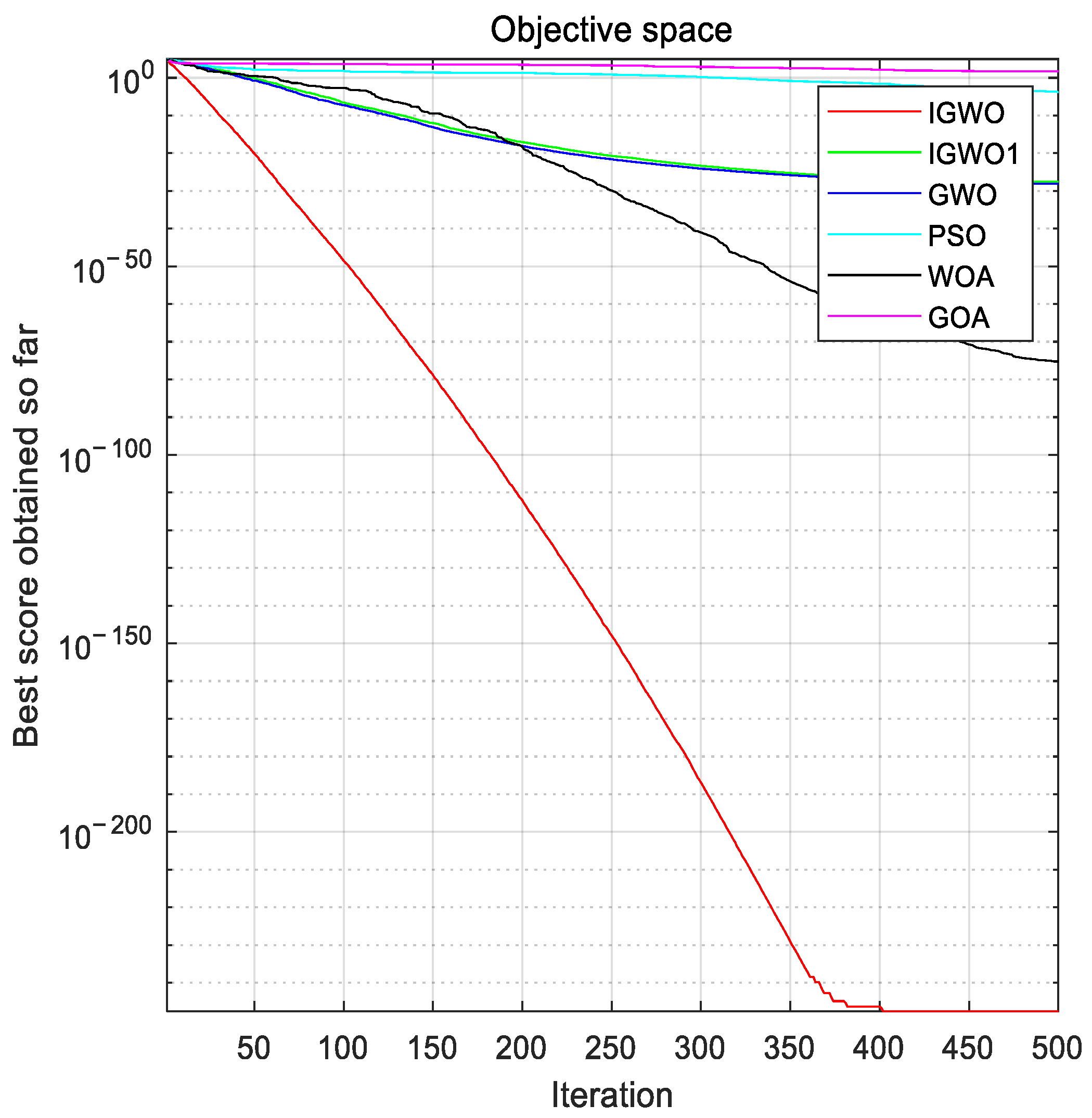
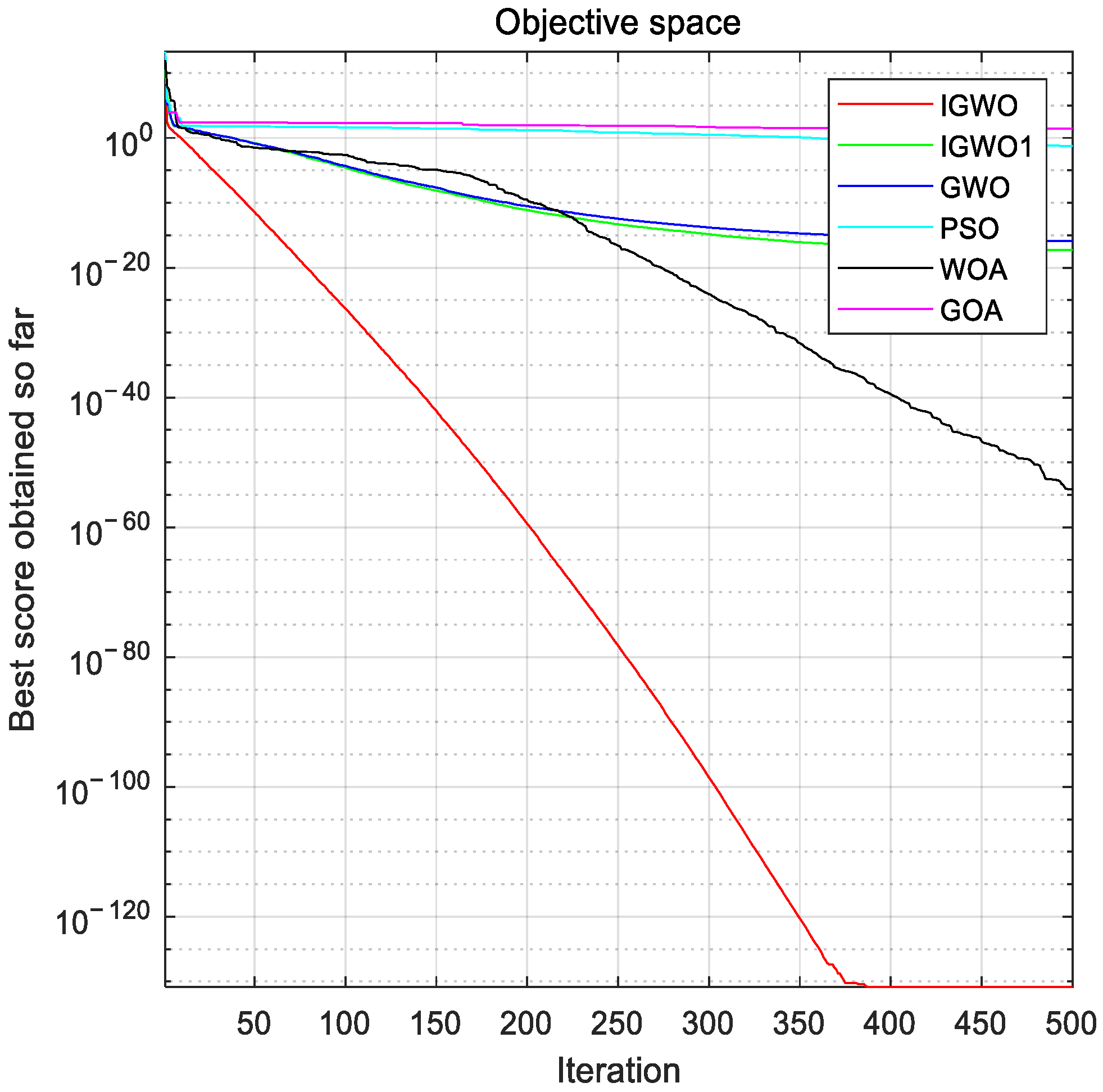
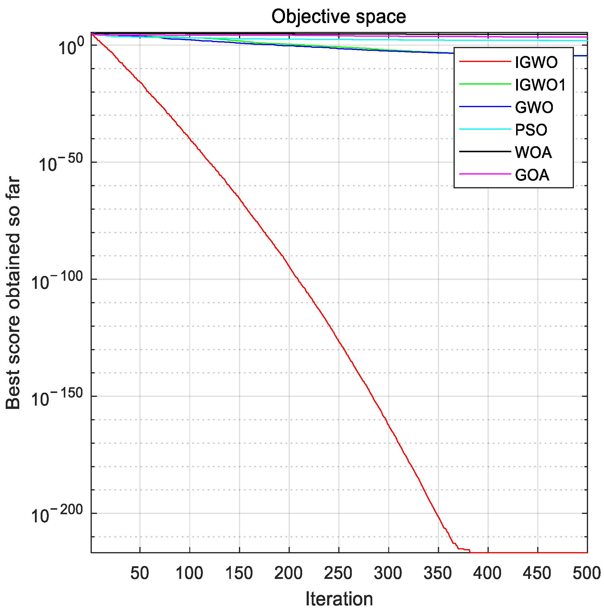
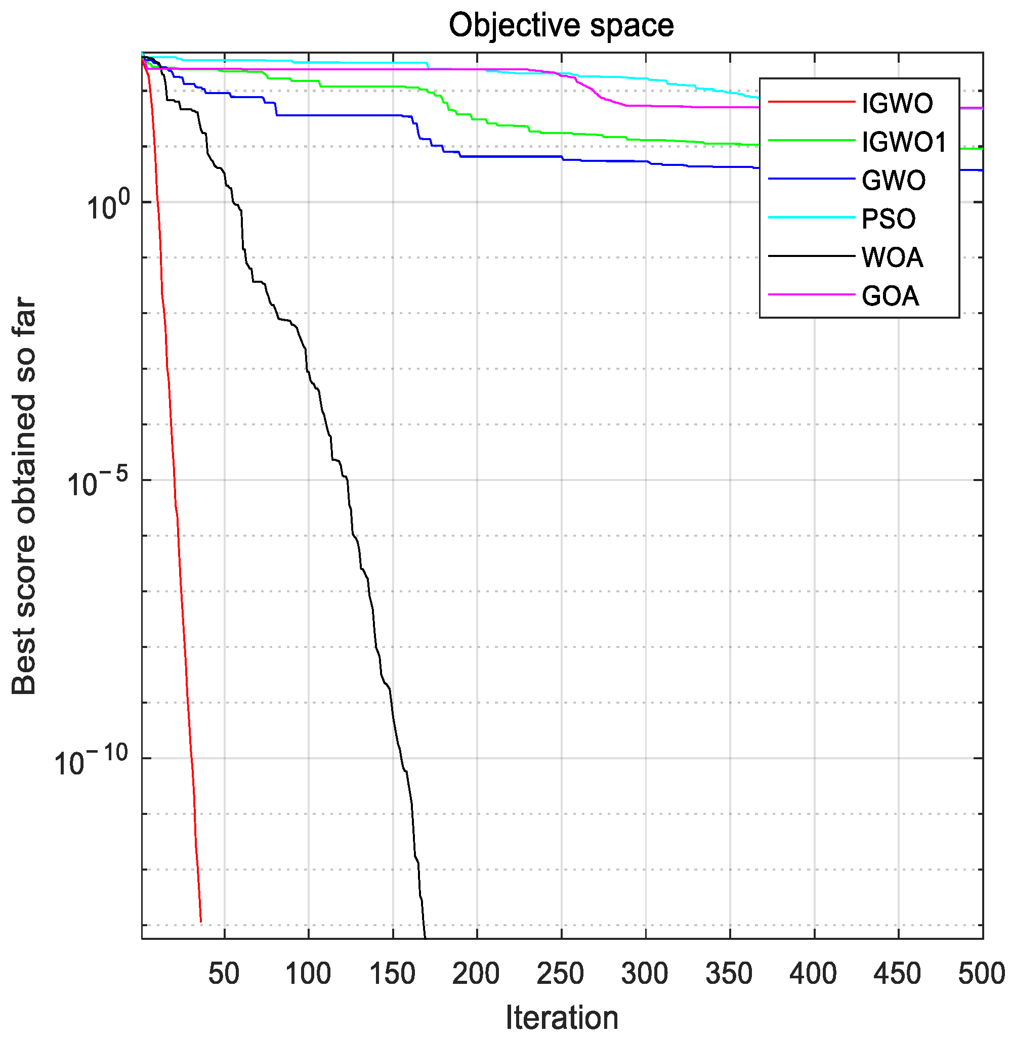
The performance of the optimization algorithm should be evaluated in terms of convergence accuracy, convergence speed, robustness, etc. Therefore, the results of 30 independent runs of different algorithms on functions in different dimensions of 30, 50, and 100 were evaluated. The information of the mean, best value, and standard deviation of the results is shown in

Table 3. The statistics data of 30 runs of the benchmarks of 30 dimension.

NO.	Statistics	PSO	WOA	GOA	GWO	IGWO1	IGWO
F1	Mean	2.82 × 10−15	2.92 × 10−304	1.68 × 10−1	1.36 × 10−121	1.11 × 10−124	0.00
	Std	9.89 × 10−15	0.00	1.89 × 10−1	3.76 × 10−121	2.21 × 10−124	0.00
	Best	3.88 × 10−21	0.00	7.72 × 10−3	1.52 × 10−126	4.95 × 10−129	0.00
	Runtime(s)	1.74 × 10−1	1.69 × 10−1	7.76 × 10	2.42 × 10−1	1.32	3.41 × 10−1
	Winner	1	0	1	1	1
F2	Mean	1.19 × 10−7	1.70 × 10−212	9.93 × 10−1	8.32 × 10−71	4.08 × 10−75	0.00
	Std	2.56 × 10−7	0.00	8.48 × 10−1	1.23 × 10−70	1.13 × 10−74	0.00
	Best	2.05 × 10−10	2.53 × 10−223	4.13 × 10−1	7.36 × 10−73	5.02 × 10−77	0.00
	Runtime(s)	1.60 × 10−1	1.62 × 10−1	7.75 × 10	2.48 × 10−1	1.33	3.64 × 10−1
	Winner	1	1	1	1	1
F3	Mean	1.16	6.93 × 103	9.31 × 102	4.52 × 10−31	4.77 × 10−22	0.00
	Std	6.66 × 10−1	6.00 × 103	1.72 × 102	2.41 × 10−30	2.60 × 10−21	0.00
	Best	2.79 × 10−1	3.57 × 10	7.00 × 102	4.94 × 10−42	1.43 × 10−28	0.00
	Runtime(s)	4.86 × 10−1	4.67 × 10−1	7.76 × 10	5.73 × 10−1	1.99	6.81 × 10−1
	Winner	1	1	1	1	1
F4	Mean	4.38 × 10	2.64 × 10	2.19 × 102	2.67 × 10	2.16 × 10	2.87 × 10
	Std	2.82 × 10	5.31 × 10−1	1.48 × 102	8.26 × 10−1	4.34 × 10−1	2.54 × 10−1
	Best	1.08 × 10	2.57 × 10	3.97 × 10	2.49 × 10	2.07 × 10	2.81 × 10
	Runtime(s)	1.95 × 10−1	1.99 × 10−1	7.77 × 10	2.82 × 10−1	1.40	3.76 × 10−1
	Winner	0	−1	1	−1	0
F5	Mean	3.02 × 10−2	7.44 × 10−4	9.55 × 10−3	4.11 × 10−4	6.50 × 10−4	2.12 × 10−5
	Std	9.44 × 10−3	8.77 × 10−4	5.48 × 10−3	2.22 × 10−4	3.03 × 10−4	1.91 × 10−5
	Best	1.66 × 10−2	2.52 × 10−5	4.12 × 10−3	1.39 × 10−4	2.59 × 10−4	1.99 × 10−7
	Runtime(s)	3.59 × 10−1	3.63 × 10−1	7.81 × 10	4.61 × 10−1	1.78	5.63 × 10−1
	Winner	1	1	1	1	1
F6	Mean	4.22 × 10	0.00	9.28 × 10	2.15 × 10−1	1.41 × 10	0.00
	Std	9.18	0.00	4.07 × 10	1.18	4.89	0.00
	Best	2.79 × 10	0.00	6.72 × 10	0.00	2.99	0.00
	Runtime(s)	1.86 × 10−1	1.66 × 10−1	7.83 × 10	2.54 × 10−1	1.39	3.50 × 10−1
	Winner	1	−1	1	1	1
F7	Mean	3.88 × 10−8	3.52 × 10−15	4.09	9.44 × 10−15	7.43 × 10−15	3.88 × 10−15
	Std	7.75 × 10−8	2.59 × 10−15	1.10	2.91 × 10−15	6.49 × 10−16	6.49 × 10−16
	Best	8.85 × 10−12	4.44 × 10−16	3.23	7.55 × 10−15	4.00 × 10−15	4.44 × 10−16
	Runtime(s)	1.78 × 10−1	1.68 × 10−1	7.84 × 10	2.52 × 10−1	1.35	3.51 × 10−1
	Winner	1	−1	1	1	1
F8	Mean	7.64 × 10−3	2.01 × 10−3	5.09 × 10−1	1.71 × 10−3	3.88 × 10−3	0.00
	Std	7.85 × 10−3	7.89 × 10−3	1.12 × 10−1	6.03 × 10−3	8.52 × 10−3	0.00
	Best	0.00	0.00	3.92 × 10−1	0.00	0.00	0.00
	Runtime(s)	2.02 × 10−1	1.95 × 10−1	7.88 × 10	2.78 × 10−1	1.42	3.78 × 10−1
	Winner	1	1	1	1	1

,

Table 4. The statistics data of 30 runs of the benchmarks of 50 dimension.

NO.	Statistics	PSO	WOA	GOA	GWO	IGWO1	IGWO
F1	Mean	3.95 × 10−7	1.54 × 10−295	6.12 × 10	1.51 × 10−90	6.17 × 10−92	0.00
	Std	6.80 × 10−7	0.00	1.21 × 10	7.63 × 10−90	1.13 × 10−91	0.00
	Best	9.11 × 10−10	0.00	4.89 × 10	1.96 × 10−94	2.46 × 10−94	0.00
	Runtime(s)	1.96 × 10−1	1.98 × 10−1	1.30 × 102	3.74 × 10−1	1.53	5.36 × 10−1
	Winner	1	0	1	1	1
F2	Mean	5.54 × 10−3	1.36 × 10−207	2.42 × 10	1.31 × 10−53	1.90 × 10−56	0.00
	Std	1.19 × 10−2	0.00	2.80 × 10	9.31 × 10−54	2.89 × 10−56	0.00
	Best	9.86 × 10−5	2.30 × 10−229	4.54	2.58 × 10−54	3.95 × 10−58	0.00
	Runtime(s)	2.11 × 10−1	1.87 × 10−1	1.31 × 102	3.81 × 10−1	1.55	5.90 × 10−1
	Winner	1	1	1	1	1
F3	Mean	1.78 × 102	6.60 × 104	8.30 × 103	6.18 × 10−17	6.99 × 10−7	0.00
	Std	5.74 × 10	2.76 × 104	3.79 × 103	2.63 × 10−16	1.94 × 10−6	0.00
	Best	8.16 × 10	1.57 × 104	4.27 × 103	2.17 × 10−24	6.55 × 10−12	0.00
	Runtime(s)	7.49 × 10−1	7.22 × 10−1	1.27 × 102	9.69 × 10−1	2.66	1.13
	Winner	1	1	1	1	1
F4	Mean	1.08 × 102	4.66 × 10	1.11 × 104	4.69 × 10	4.21 × 10	4.88 × 10
	Std	4.64 × 10	3.32 × 10−1	6.66 × 103	7.87 × 10−1	3.68 × 10−1	2.50 × 10−1
	Best	3.34 × 10	4.60 × 10	2.88 × 103	4.56 × 10	4.17 × 10	4.81 × 10
	Runtime(s)	2.35 × 10−1	2.23 × 10−1	1.26 × 102	4.10 × 10−1	1.64	5.67 × 10−1
	Winner	0	−1	1	−1	0
F5	Mean	1.59 × 10−1	8.84 × 10−4	2.01 × 10−2	4.86 × 10−4	1.30 × 10−3	2.02 × 10−5
	Std	5.36 × 10−2	1.25 × 10−3	7.63 × 10−3	2.37 × 10−4	4.94 × 10−4	2.11 × 10−5
	Best	8.39 × 10−2	2.63 × 10−5	1.11 × 10−2	1.05 × 10−4	5.77 × 10−4	1.45 × 10−6
	Runtime(s)	5.57 × 10−1	5.19 × 10−1	1.25 × 102	7.51 × 10−1	2.25	8.86 × 10−1
	Winner	1	1	1	1	1
F6	Mean	1.15 × 102	0.00	1.52 × 102	0.00	2.76 × 10	0.00
	Std	2.60 × 10	0.00	5.56 × 10	0.00	1.14 × 10	0.00
	Best	5.77 × 10	0.00	1.01 × 102	0.00	1.02 × 10	0.00
	Runtime(s)	2.58 × 10−1	1.91 × 10−1	1.26 × 102	3.75 × 10−1	1.62	5.43 × 10−1
	Winner	1	−1	1	−1	1
F7	Mean	2.46 × 10−1	4.00 × 10−15	8.29	1.49 × 10−14	1.37 × 10−14	4.00 × 10−15
	Std	5.65 × 10−1	2.64 × 10−15	1.71	2.27 × 10−15	2.07 × 10−15	0.00
	Best	1.33 × 10−5	4.44 × 10−16	5.98	7.55 × 10−15	7.55 × 10−15	4.00 × 10−15
	Runtime(s)	2.43 × 10−1	1.92 × 10−1	1.26 × 102	3.73 × 10−1	1.55	5.41 × 10−1
	Winner	1	−1	1	1	1
F8	Mean	2.55 × 10−3	5.87 × 10−3	1.23	7.17 × 10−4	1.56 × 10−3	0.00
	Std	4.91 × 10−3	1.84 × 10−2	3.76 × 10−2	2.73 × 10−3	4.45 × 10−3	0.00
	Best	8.91 × 10−11	0.00	1.17	0.00	0.00	0.00
	Runtime(s)	2.62 × 10−1	2.51 × 10−1	1.26 × 102	4.12 × 10−1	1.64	5.76 × 10−1
	Winner	1	1	1	1	1

and

Table 5. The statistics data of 30 runs of the benchmarks of 100 dimension.

NO.	Statistics	PSO	WOA	GOA	GWO	IGWO1	IGWO
F1	Mean	1.72 × 10−1	1.22 × 10−297	2.91 × 103	8.92 × 10−63	2.52 × 10−61	0.00
	Std	2.30 × 10−1	0.00	7.08 × 102	1.65 × 10−62	4.77 × 10−61	0.00
	Best	2.15 × 10−2	0.00	1.88 × 103	6.56 × 10−65	4.19 × 10−64	0.00
	Runtime(s)	3.13 × 10−1	2.59 × 10−1	2.57 × 102	6.45 × 10−1	2.01	1.00
	Winner	1	0	1	1	1
F2	Mean	2.34	3.07 × 10−207	7.75 × 10	9.02 × 10−38	3.11 × 10−39	0.00
	Std	1.07	0.00	2.35 × 10	6.26 × 10−38	2.30 × 10−39	0.00
	Best	6.05 × 10−1	8.18 × 10−222	5.57 × 10	2.86 × 10−38	3.46 × 10−40	0.00
	Runtime(s)	2.92 × 10−1	2.43 × 10−1	2.57 × 102	6.62 × 10−1	2.03	1.05
	Winner	1	1	1	1	1
F3	Mean	6.11 × 103	6.76 × 10−5	6.84 × 10−4	5.48 × 10−3	5.57 × 10	0.00
	Std	1.60 × 103	1.22 × 105	2.14 × 104	1.96 × 10−2	5.55 × 10	0.00
	Best	3.24 × 103	3.39 × 105	3.86 × 104	6.27 × 10−10	2.42	0.00
	Runtime(s)	1.46	1.43	2.60 × 102	1.92	4.46	2.27
	Winner	1	1	1	1	1
F4	Mean	5.76 × 102	9.69 × 10	1.11 × 106	9.73 × 10	9.34 × 10	9.88 × 10
	Std	1.57 × 102	5.97 × 10−1	6.30 × 105	9.18 × 10−1	1.46	2.01 × 10−1
	Best	3.66 × 102	9.63 × 10	7.94 × 105	9.49 × 10	9.18 × 10	9.81 × 10
	Runtime(s)	3.28 × 10−1	2.92 × 10−1	2.66 × 102	7.05 × 10−1	2.10	1.03
	Winner	1	−1	1	−1	0
F5	Mean	1.00 × 103	1.05 × 10−3	2.55 × 10−1	9.83 × 10−4	3.09 × 10−3	2.43 × 10−5
	Std	4.69 × 102	1.46 × 10−3	1.07 × 10−1	4.61 × 10−4	8.45 × 10−4	2.41 × 10−5
	Best	5.51	6.68 × 10−5	1.62 × 10−1	4.44 × 10−4	1.71 × 10−3	3.03 × 10−7
	Runtime(s)	9.73 × 10−1	9.13 × 10−1	2.59 × 102	1.36	3.48	1.70
	Winner	1	1	1	1	1
F6	Mean	3.98 × 102	0.00	3.11 × 102	3.79 × 10−14	6.13 × 10	0.00
	Std	6.40 × 10	0.00	8.40 × 10	8.08 × 10−14	3.74 × 10	0.00
	Best	2.83 × 102	0.00	1.91 × 102	0.00	6.44	0.00
	Runtime(s)	4.05 × 10−1	2.54 × 10−1	2.62 × 102	6.79 × 10−1	2.21	1.02
	Winner	1	−1	1	1	1
F7	Mean	1.85	3.29 × 10−15	1.27 × 10	2.83 × 10−14	2.70 × 10−14	4.00 × 10−15
	Std	4.45 × 10−1	2.54 × 10−15	7.32 × 10−1	4.28 × 10−15	3.46 × 10−15	0.00
	Best	3.66 × 10−1	4.44 × 10−16	1.21 × 10	1.82 × 10−14	2.18 × 10−14	4.00 × 10−15
	Runtime(s)	4.20 × 10−1	2.58 × 10−1	2.52 × 102	6.38 × 10−1	2.09	1.01
	Winner	1	−1	1	1	1
F8	Mean	5.43 × 10−3	0.00	1.70 × 10	6.04 × 10−4	2.38 × 10−3	0.00
	Std	6.75 × 10−3	0.00	2.21	2.30 × 10−3	7.09 × 10−3	0.00
	Best	2.12 × 10−4	0.00	1.32 × 10	0.00	0.00	0.00
	Runtime(s)	3.92 × 10−1	2.91 × 10−1	2.53 × 102	6.81 × 10−1	2.18	1.06
	Winner	1	−1	1	1	1

, and the comparison graphs of the convergence curves of the six algorithms for the test functions of 30 dimensions are shown in Figure 4, Figure 5, Figure 6, Figure 7, Figure 8, Figure 9, Figure 10 and Figure 11.

In Figure 4, Figure 5, Figure 6, Figure 7, Figure 8, Figure 9, Figure 10 and Figure 11, iterative convergence curves are plotted for eight typical functions representing the full range of features from F1 to F8. It can be seen that the convergence curves of the IGWO show a strong exploration and exploitation capability overall compared to other algorithms. In the F1, F2, F3, F6, and F8 test plots, it can be seen that the convergence curves of the algorithm change more drastically, which indicates that the improved parameters A and C and the updated Formula (19) provide better solutions for the algorithm and speed up the convergence of the algorithm when dealing with single-mode and multi-mode problems. In the F4, F5, and F7 test plots, it can be seen that the convergence curve of the algorithm has an obvious turn in the iterative process, which indicates that the enhanced population diversity of the improved algorithm makes the convergence accuracy of the algorithm show a significant improvement compared with most other algorithms when dealing with single-mode and multi-mode problems, further verifying the detection capability of the IGWO. From the overall test results, it is clear that the first half of the improved algorithm’s curve has completed convergence and that the convergence accuracy is closer to the optimal value, illustrating the important role of the proposed algorithm-improvement mechanism in the global search. In addition, compared with other algorithms, the IGWO had a faster convergence speed and maintained a better convergence accuracy, thus verifying the effectiveness of the improved gray wolf algorithm.

In addition, the comparisons of various stability metrics of the six algorithms tested against eight functions in three different dimensions, including the mean, standard deviation, optimal value, and running time, are presented in Table 3, Table 4 and Table 5, respectively. The meaning of the indicator Winner in the table is the superiority and inferiority of IGWO compared with the test results of other algorithms. Winner 1, 0, and −1 respectively mean that IGWO is superior to, comparable to, or worse than the other algorithms on the whole. First, it can be seen from the table that the performance of the algorithm did not change much as the function dimension increased, and the convergence accuracy of the algorithm improved, which depends on the improvement of the algorithm’s exploration capability. Second, the overall test effect of the IGWO algorithm on the unimodal reference function is obviously better than that of other algorithms. Although the effect of the IGWO algorithm on F4 is not as good as that of the WOA and GWO algorithms, the difference of indicators is not large, and the results are still better than other algorithms. In addition, the IGWO algorithm showed good results in testing multimodal benchmark functions, except for the F6 and F7 test results, which were slightly worse than those of the WOA, while the other functional test indicators were better than most algorithms. Finally, compared with the original gray wolf algorithm, the improved gray wolf algorithm has improved all the indicators of the test functions. Only in test F4, the improved gray wolf algorithm was inferior to the original gray wolf algorithm, and the other test function indicators were basically better than the original gray wolf algorithm. Thus, on the whole, IGWO won 98 out of 120 comparisons, thus verifying the effectiveness of the improved gray wolf algorithm.

In summary, the IGWO has excellent performance in testing benchmark problems, especially compared with the original gray wolf algorithm; its exploration and exploitation capability has been greatly enhanced, which avoids the algorithm falling into local optimal solutions to a certain extent, but it needs to be strengthened in solving multimodal benchmark problems.

5.2. Results Analysis of IGWO Test Dynamic Economic Dispatch Model

In order to verify the reliability of the algorithm and constraint treatment proposed in this paper in solving the economic dispatch problem, three cases of different sizes of the single-objective dynamic economic dispatch model were considered, namely Case 1: 5 generating units; Case 2: 10 generating units; and Case 3: 15 generating units [41]. The scheduling period was T = 24 h and the valve point effect and transmission loss constraints were considered for each case, with the corresponding B-factors taken from the studies of Qian and Mohammadi et al. [41,42]. The maximum number of evaluations of the algorithm was D × 10,000, with D representing the dimensionality of the decision variables; in addition, the maximum allowable error at each moment in the process of repairing infeasible solutions was 0.001, and to avoid chance, each case was run 30 times independently. The experiments were simulated in MATLAB software.

Calculation Results and Comparison

To make the comparison results look more intuitive, the optimal solutions of the test results for GWO and IGWO under the three cases are summarized in

Table 6. Comparison of results with different algorithms for Case I.

Algorithms	Fuel Costs ($)	Power Balance Constraint Violations (MW)
SA [9]	$47.36 K	1.10 × 10−1
PS [43]	$46.53 K	3.00 × 10−2
ABC [44]	$44.05 K	2.00 × 10−3
AIS [45]	$44.39 K	1.00 × 10−3
PSO-SQP [46]	$43.26 K	1.00 × 10−3
CMAES [47]	$45.54 K	193.18
DHS [48]	$45.89 K	1.00 × 10−4
MHS [48]	$45.50 K	1.00 × 10−4
MBDE [49]	$48.32 K	1.30 × 10−5
MSL [50]	$48.66 K	2.00 × 10−3
GWO	$47.15 K	1.26 × 10−5
IGWO	$43.16 K	2.51 × 10−4

,

Table 7. Comparison of results with different algorithms for Case II.

Algorithms	Fuel Costs ($)	Power Balance Constraint Violations (MW)
SPS-DE [29]	$2.47 M	2.00 × 10−3
DE-SQP [46]	$2.47 M	193.18
PSO-SQP [46]	$2.47 M	184.22
MBDE [49]	$2.60 M	1.30 × 10−5
HCRO [51]	$2.48 M	1.00
CRO [51]	$2.48 M	1.00 × 10−3
IBFA [52]	$2.48 M	2.00 × 10−3
AIS [53]	$2.52 M	1.10 × 10−1
PSO [53]	$2.57 M	1.00 × 10−3
EP [53]	$2.59 M	3.00 × 10−2
GWO	$2.57 M	−2.79 × 10−6
IGWO	$2.45 M	−2.30 × 10−4

and

Table 8. Comparison of results with different algorithms for Case III.

Algorithms	Fuel Costs ($)	Power Balance Constraint Violations (MW)
GWO	$0.69 M	2.80 × 10−5
IGWO	$0.65 M	3.19 × 10−5

, including the feasibility verification of the optimal solutions and the fuel costs corresponding to the optimal solutions, and the optimal solutions for each case tested by other algorithms proposed in the literature are also listed for comparison. In addition, the power output information of the optimal solutions for GWO and IGWO under Case 1 and Case 2 is shown in

Table 9. The best results of GWO for Case I.

Hour	P (MW)					PD	V (t)
	P1	P2	P3	P4	P5
1	12.25	88.02	40.44	49.71	223.59	410	7.88 × 10−5
2	10.00	104.40	48.22	42.96	233.96	435	−1.26 × 10−4
3	18.33	96.79	55.55	81.21	228.25	475	−3.37 × 10−5
4	14.91	92.12	88.77	107.29	233.06	530	−2.44 × 10−5
5	11.81	98.35	98.52	122.16	233.93	558	−7.37 × 10−5
6	31.76	100.32	118.32	129.44	236.05	608	−2.52 × 10−5
7	47.11	105.57	114.15	127.93	239.60	626	−9.90 × 10−5
8	66.14	90.01	125.95	142.86	238.03	654	1.28 × 10−4
9	65.10	100.23	119.99	136.35	278.55	690	−2.09 × 10−5
10	42.70	102.40	159.99	167.86	241.44	704	5.94 × 10−5
11	46.83	96.86	136.10	205.46	245.71	720	1.22 × 10−4
12	58.50	96.96	156.68	211.01	228.32	740	1.12 × 10−4
13	35.60	110.95	130.49	208.19	229.32	704	9.50 × 10−5
14	35.13	106.97	122.40	207.76	227.90	690	1.54 × 10−4
15	11.51	101.11	111.68	207.48	231.49	654	1.62 × 10−5
16	10.31	78.21	114.00	191.03	193.64	580	8.36 × 10−5
17	17.54	66.52	114.02	141.06	225.47	558	−3.23 × 10−5
18	15.18	95.80	111.15	164.71	229.08	608	4.36 × 10−5
19	17.29	100.83	109.26	213.73	222.15	654	8.82 × 10−5
20	34.29	103.51	128.47	203.11	245.17	704	−2.01 × 10−6
21	19.89	101.37	124.88	211.07	232.71	680	2.80 × 10−5
22	14.80	108.16	101.86	166.69	221.41	605	−1.5 × 10−4
23	14.34	93.61	72.61	130.51	222.05	527	−1.34 × 10−4
24	10.54	64.00	42.31	108.10	243.00	463	1.42 × 10−5

The total fuel cost is $47.15 K.

,

Table 10. The best results of IGWO for Case I.

Hour	P (MW)					PD	V (t)
	P1	P2	P3	P4	P5
1	11.04	99.13	30.02	124.93	139.85	410	3.24 × 10−4
2	10.81	98.53	30.00	125.38	189.85	435	1.63 × 10−4
3	11.29	98.58	32.95	124.97	229.58	475	2.04 × 10−4
4	15.24	100.57	72.95	125.00	229.59	530	3.13 × 10−4
5	11.49	98.56	112.58	126.51	229.61	558	3.04 × 10−4
6	11.19	98.90	112.81	176.51	230.57	608	2.69 × 10−4
7	11.83	98.77	112.80	209.86	229.62	626	2.09 × 10−4
8	29.01	98.44	112.77	209.90	229.59	654	3.38 × 10−4
9	58.85	98.60	112.70	209.88	231.32	690	2.64 × 10−4
10	75.00	101.70	113.06	209.89	229.79	704	3.22 × 10−4
11	74.98	99.34	113.35	209.89	229.59	720	3.06 × 10−4
12	75.00	99.79	113.25	209.86	229.51	740	2.36 × 10−4
13	75.00	99.34	112.87	210.08	233.56	704	1.64 × 10−4
14	75.00	99.18	112.91	210.03	229.80	690	3.76 × 10−4
15	45.98	98.57	112.75	209.99	229.58	654	1.97 × 10−4
16	15.98	84.89	112.61	209.73	229.47	580	2.52 × 10−4
17	10.04	68.26	112.50	209.78	227.52	558	3.51 × 10−4
18	11.35	98.26	113.19	209.85	229.55	608	2.90 × 10−4
19	10.91	80.57	112.77	209.78	229.54	654	4.14 × 10−4
20	11.35	98.63	112.80	209.92	229.54	704	2.14 × 10−4
21	12.89	98.62	112.64	209.83	222.55	680	2.97 × 10−4
22	11.91	98.97	112.73	209.92	229.54	605	1.35 × 10−4
23	10.00	103.18	112.49	198.02	179.56	527	8.73 × 10−5
24	10.05	98.69	112.70	148.55	139.83	463	−6.24 × 10−6

The total fuel cost is $43.16 K.

,

Table 11. The best results of GWO for Case II.

Hour	P (MW)										PD	V (t)
	P1	P2	P3	P4	P5	P6	P7	P8	P9	P10
1	153.18	214.84	91.13	149.57	132.95	97.39	65.73	67.96	56.86	26.71	1036	−8.87 × 10−5
2	157.15	142.40	131.37	190.03	176.47	86.80	71.41	80.46	47.63	48.95	1110	−5.72 × 10−6
3	155.42	166.76	147.75	227.63	206.09	95.73	90.22	96.33	53.93	47.24	1258	−2.63 × 10−5
4	210.48	180.18	193.56	211.73	243.00	103.43	100.29	105.18	50.03	44.91	1406	−2.26 × 10−5
5	171.86	141.18	270.05	245.39	221.12	115.11	124.95	120.00	59.89	50.40	1480	4.40 × 10−5
6	214.15	195.01	287.59	245.99	235.30	150.11	130.00	108.24	64.19	46.45	1628	1.91 × 10−5
7	211.51	199.89	334.27	287.07	228.55	144.05	127.18	112.71	60.13	50.47	1702	1.28 × 10−4
8	244.84	275.78	329.58	264.17	221.12	158.16	120.59	106.07	73.39	42.01	1776	−8.22 × 10−5
9	314.48	304.86	323.73	293.00	240.24	148.63	130.00	112.31	78.30	49.89	1924	−1.70 × 10−4
10	334.91	381.47	322.32	295.97	237.34	159.35	126.58	118.17	76.36	49.80	2022	9.48 × 10−5
11	369.55	427.22	326.86	300.00	241.98	157.36	130.00	119.30	71.97	50.21	2106	−4.51 × 10−5
12	408.14	459.12	333.94	287.46	233.37	155.82	124.59	117.62	71.37	52.24	2150	1.14 × 10−4
13	366.35	395.72	331.29	297.88	237.63	155.24	129.52	116.07	78.76	48.63	2072	−4.81 × 10−5
14	294.13	360.81	328.01	280.25	243.00	139.51	120.31	118.66	75.72	35.66	1924	−2.86 × 10−5
15	232.02	300.52	326.20	261.02	230.17	146.59	127.11	106.23	58.88	47.20	1776	4.79 × 10−5
16	166.10	239.41	292.04	261.42	236.24	131.60	121.90	81.36	38.10	30.74	1554	1.30 × 10−4
17	170.79	250.74	237.06	245.24	215.07	105.03	125.07	99.60	25.29	47.07	1480	−5.29 × 10−5
18	202.55	238.83	284.46	266.95	235.64	123.47	120.84	114.72	49.77	40.29	1628	6.16 × 10−5
19	234.62	231.96	333.60	299.92	242.24	155.95	124.31	108.70	56.75	47.05	1776	−5.84 × 10−5
20	310.87	311.96	340.00	300.00	243.00	160.00	127.44	120.00	78.90	54.79	1972	−1.54 × 10−5
21	290.11	303.56	340.00	292.08	235.72	159.51	128.79	119.18	74.42	51.60	1924	−1.05 × 10−4
22	221.69	237.63	281.14	284.84	215.01	124.87	129.68	92.44	57.28	33.15	1628	3.69 × 10−5
23	153.64	197.76	248.43	254.99	168.62	108.30	109.86	77.12	35.60	10.45	1332	4.54 × 10−5
24	150.00	142.77	236.65	205.19	166.19	111.10	84.95	64.88	23.60	24.28	1184	−4.06 × 10−5

The total fuel cost is $2.57 M.

and

Table 12. The best results of IGWO for Case II.

Hour	P (MW)										PD	V (t)
	P1	P2	P3	P4	P5	P6	P7	P8	P9	P10
1	150.00	135.00	92.13	120.16	222.60	122.42	129.54	119.94	20.00	10.00	1036	−8.99 × 10−5
2	150.00	135.00	167.77	121.16	222.64	122.38	129.67	120.00	20.06	10.00	1110	−2.67 × 10−6
3	150.01	135.00	185.37	171.16	222.69	149.46	129.70	120.00	49.71	40.00	1258	1.23 × 10−4
4	150.00	135.00	265.21	219.52	233.40	159.94	129.88	119.93	51.94	43.77	1406	1.04 × 10−5
5	150.03	135.01	297.50	247.88	223.18	160.00	129.73	120.00	79.99	43.43	1480	−6.04 × 10−5
6	150.06	135.95	340.00	297.88	243.00	160.00	130.00	120.00	80.00	54.97	1628	−4.35 × 10−5
7	150.73	215.88	339.88	300.00	243.00	160.00	130.00	120.00	80.00	55.00	1702	3.56 × 10−5
8	197.50	222.38	340.00	300.00	243.00	160.00	130.00	119.99	80.00	55.00	1776	−4.79 × 10−4
9	229.48	302.32	340.00	299.99	243.00	160.00	130.00	120.00	80.00	55.00	1924	−1.09 × 10−4
10	301.03	309.66	340.00	300.00	242.99	159.99	130.00	120.00	80.00	55.00	2022	−7.35 × 10−5
11	324.58	389.66	340.00	300.00	243.00	160.00	130.00	120.00	80.00	55.00	2106	−3.59 × 10−5
12	353.15	396.77	340.00	300.00	243.00	160.00	130.00	120.00	80.00	55.00	2150	−9.42 × 10−4
13	292.77	382.31	340.00	300.00	243.00	160.00	130.00	120.00	80.00	55.00	2072	2.63 × 10−5
14	225.62	302.31	340.00	300.00	243.00	160.00	130.00	120.00	80.00	55.00	1924	8.51 × 10−6
15	191.02	222.34	340.00	300.00	242.96	159.99	130.00	119.99	80.00	54.95	1776	−8.83 × 10−5
16	150.01	142.36	297.95	300.00	241.41	159.98	130.00	119.99	80.00	43.43	1554	−2.17 × 10−4
17	150.00	135.00	302.08	251.63	242.81	160.00	129.71	119.99	52.10	43.44	1480	6.49 × 10−5
18	150.19	142.29	339.99	299.96	242.99	159.99	129.88	119.99	80.00	55.00	1628	6.95 × 10−5
19	207.41	222.29	340.00	300.00	243.00	160.00	130.00	120.00	80.00	55.00	1776	−9.91 × 10−4
20	255.59	302.14	340.00	300.00	242.99	160.00	130.00	119.99	80.00	55.00	1972	−9.32 × 10−4
21	226.43	292.46	340.00	300.00	243.00	160.00	130.00	120.00	80.00	55.00	1924	−8.91 × 10−4
22	150.00	213.14	304.78	299.93	242.86	160.00	130.00	120.00	80.00	43.43	1628	−0.01 × 10−1
23	150.00	135.00	234.43	250.00	223.54	123.16	129.71	119.99	51.57	13.47	1332	6.82 × 10−5
24	150.00	135.00	163.63	200.16	223.02	122.73	129.63	119.99	21.63	10.01	1184	3.67 × 10−5

The total fuel cost is $2.45 M.

, and the stacked histograms of the optimal output results for GWO and IGWO under Case 3 are shown in Figure 12 and Figure 13.

Table 6, Table 7 and Table 8 show the comparison of a series algorithms from the literature with IGWO under three cases, including a comparison with the original GWO algorithm. As can be seen from the table, first, the optimal fuel costs solved by the IGWO are $43.16 K, $2.45 M, and $0.65 M, which are better than the test results of all other algorithms proposed in the literature, which indicates that the innovative method proposed in this paper is effective. On the one hand, the chaotic initialization of the algorithm population makes the algorithm enhance a certain exploration capability in the initial stage, which can help avoid the algorithm falling too quickly into a local optimum; on the other hand, the introduction of the nonlinear convergence factor accelerates the convergence speed of the algorithm; furthermore, the adaptive strategy of the weight of the position update equation also improves the convergence accuracy of the algorithm and further enhances the exploration and exploitation capability of the algorithm. Second, the equation constraint violations of the IGWO are 2.51 × 10⁻⁴, −2.30 × 10⁻⁴, and 3.19 × 10⁻⁵, which are smaller than the constraint violations of most other algorithms, and the constraint violations under each case are smaller than 0.001, which illustrates the feasibility of the coarse and fine tuning, and further verifies that the hybrid constraint-processing method proposed in this paper is effective and thus greatly reduces the constraint violations.

In addition, according to Table 9, Table 10, Table 11 and Table 12, comparing the power output information of the IGWO and GWO in the two cases, the GWO and IGWO ran for 18.32 s and 18.82 s on test Case 1, respectively, and 45.68 s and 45.97 s, respectively, on test Case 2. It is found that the optimal solution of the IGWO is significantly better than that of the GWO, which shows that although the constraints are also satisfied, the IGWO has higher exploration capability and convergence accuracy due to the improvement of the population initialization and position update strategy, and also as seen in the stacked histograms of Figure 12 and Figure 13 (Case 3), the GWO and IGWO ran for 83.84 s and 84.24 s, respectively, on test Case 3. It is worth noting here that the disaster of dimension needs to be considered in the case of solving Case 3 (Unit 15). From the results of test Case 3, the operation time of the improved algorithm is shorter, and the obtained fuel cost is also better than in other algorithms, which indicates that the improved algorithm also shows a faster convergence speed and better convergence accuracy for solving high-dimensional problems. In addition, it can be seen from Figure 12 and Figure 13 that the improved algorithm solves the array variance less, which indicates that the improved algorithm has a more stable performance in solving high-dimensional problems, and thus the method proposed in this paper can better reduce the impact of high-dimensional space. In summary, IGWO has an advantage over other algorithms when applied to the DED problem.

6. Conclusions

In order to alleviate the current energy problem and find an effective method to solve the DED problem, an improved gray wolf optimization algorithm (IGWO) and a constraint-processing technique considering the efficiency of the unit are proposed in this paper, and it is proven by the benchmark experimental results that the proposed improving strategy does enhance the population diversity and convergence speed of the gray wolf algorithm, which makes the algorithm avoid falling into a local optimum. The test results of three other DED cases show that the proposed improved algorithm outperforms the original algorithm and other methods proposed in the literature, and that the proposed constraint-processing technique is better able to repair infeasible solutions and thus transform them into high-quality solutions. Additionally, the advantage of IGWO becomes more obvious as the number of units increases, which is of course related to the strong population diversity in the early stage of the algorithm, thus verifying the effectiveness of the proposed method in solving the DED problem in this paper.

There are still several shortcomings in this study, and more factors need to be considered for improvement in solving the DED problem, so future work will start from the following two aspects: (1) In addition to thermal power, the model should also comprehensively consider hydropower, wind power, photovoltaic power, and other power generation types, carry out multi-objective dynamic economic dispatch, and further consider the impact on the environment and ensuring, so as to meet various constraints while ensuring the minimum economic cost and environmental pollution. (2) More work needs to better address the problem of combining constraint processing techniques with swarm intelligence algorithms, by combining the two to solve a case study of the DED problem. Furthermore, how constraint processing techniques affect the performance of intelligent optimization algorithms on a practical problem should be explored.

References

- Niu, Q.; Zhang, H.; Li, K.; Irwin, G.W. An efficient harmony search with new pitch adjustment for dynamic economic dispatch. Energy 2014, 65, 25–43. [Google Scholar] [CrossRef]
- Sinha, N.; Chakrabarti, R.; Chattopadhyay, P.K. Evolutionary programming techniques for economic load dispatch. Int. J. Emerg. Electr. Power Syst. 2003, 7, 83–94. [Google Scholar] [CrossRef]
- Yang, Z.; Li, K.; Guo, Y.; Feng, S.; Niu, Q.; Xue, Y.; Foley, A. A binary symmetric based hybrid meta-heuristic method for solving mixed integer unit commitment problem integrating with significant plug-in electric vehicles. Energy 2019, 170, 889–905. [Google Scholar] [CrossRef]
- Yang, Z.; Li, K.; Niu, Q.; Xue, Y. A novel parallel-series hybrid meta-heuristic method for solving a hybrid unit commitment problem. Knowl.-Based Syst. 2017, 134, 13–30. [Google Scholar] [CrossRef]
- Liu, Z.F.; Li, L.L.; Liu, Y.W.; Liu, J.Q.; Li, H.Y.; Shen, Q. Dynamic economic emission dispatch considering renewable energy generation: A novel multi-objective optimization approach. Energy 2021, 235, 121407. [Google Scholar] [CrossRef]
- Acharya, S.; Ganesan, S.; Kumar, D.V.; Subramanian, S. A multi-objective multi-verse optimization algorithm for dynamic load dispatch problems. Knowl.-Based Syst. 2021, 231, 107411. [Google Scholar] [CrossRef]
- Shaheen, A.M.; Ginidi, A.R.; El-Sehiemy, R.A.; Elattar, E.E. Optimal Economic Power and Heat Dispatch in Cogeneration Systems Including Wind Power. Energy 2021, 225, 120263. [Google Scholar] [CrossRef]
- Holl, J.H. Genetic algorithms. Sci. Am. 1992, 267, 66–72. [Google Scholar]
- Panigrahi, C.K.; Chattopadhyay, P.K.; Chakrabarti, R.N.; Basu, M. Simulated Annealing Technique for dynamic economic dispatch. Electr. Power Compon. Syst. 2007, 34, 577–586. [Google Scholar] [CrossRef]
- Sawyerr, B.A.; Ali, M.M.; Adewumi, A.O. A comparative study of some real-coded genetic algorithms for unconstrained global optimization. Optim. Methods Softw. 2011, 26, 945–970. [Google Scholar] [CrossRef]
- Mirjalili, S.; Lewis, A. The Whale Optimization Algorithm. Adv. Eng. Softw. 2016, 95, 51–67. [Google Scholar] [CrossRef]
- Dorigo, M.; Birattari, M.; Stutzle, T. Ant Colony Optimization. IEEE Comput. Intell. Mag. 2006, 1, 28–39. [Google Scholar] [CrossRef]
- Liu, D.; Hu, Z.; Su, Q.; Liu, M. A niching differential evolution algorithm for the large-scale combined heat and power economic dispatch problem. Appl. Soft Comput. 2021, 113 Pt B, 108017. [Google Scholar] [CrossRef]
- Chávez, J.S.; Calderón, F.; No, S.T.; Centro, C. A Parallel Population Repair Genetic Algorithm for Power Economic Dispatch. Gen 2022, 1, 1–7. [Google Scholar]
- Mahdavi, M.; Kimiyaghalam, A.; Alhelou, H.H.; Javadi, M.S.; Ashouri, A.; Catalao, J.P.S. Transmission expansion planning considering power losses, expansion of substations and uncertainty in fuel price using discrete artificial bee colony algorithm. IEEE Access 2021, 9, 135983–135995. [Google Scholar] [CrossRef]
- Li, M.; Yang, S.; Zhang, M. Power supply system scheduling and clean energy application based on adaptive chaotic particle swarm optimization. Alex. Eng. J. 2021, 61, 2074–2087. [Google Scholar] [CrossRef]
- Wang, Z.; Dou, Z.; Dong, J.; Si, S.; Wang, C.; Liu, L. Optimal Dispatching of Regional Interconnection Multi-Microgrids Based on Multi-Strategy Improved Whale Optimization Algorithm. IEEJ Trans. Electr. Electron. Eng. 2022, 17, 766–779. [Google Scholar] [CrossRef]
- Mirjalili, S.; Mirjalili, S.M.; Lewis, A. Grey Wolf Optimizer. Adv. Eng. Softw. 2014, 69, 46–61. [Google Scholar] [CrossRef]
- Ge, F.; Li, K.; Xu, W. Path Planning of UAV for Oilfield Inspection Based on Improved Grey Wolf Optimization Algorithm. In Proceedings of the 2019 Chinese Control And Decision Conference (CCDC), Nanchang, China, 3–5 June 2019. [Google Scholar]
- Wang, P.; Rao, Y.; Luo, Q. An Effective Discrete Grey Wolf Optimization Algorithm for Solving the Packing Problem. IEEE Access 2020, 8, 115559–115571. [Google Scholar] [CrossRef]
- Yuan, J.; Li, C.; Wang, Q.; Han, Y.; Wang, J.; Zeren, Z.; Huang, J.; Feng, J.; Shen, X.; Wang, Y. Lightning Whistler Wave Speech Recognition Based on Grey Wolf Optimization Algorithm. Atmosphere 2022, 13, 1828. [Google Scholar] [CrossRef]
- İnaç, T.; Dokur, E.; Yüzgeç, U. A multi-strategy random weighted gray wolf optimizer-based multi-layer perceptron model for short-term wind speed forecasting. Neural Comput. Appl. 2022, 34, 14627–14657. [Google Scholar] [CrossRef]
- Song, C.; Wang, X.; Liu, Z.; Chen, H. Evaluation of axis straightness error of shaft and hole parts based on improved grey wolf optimization algorithm. Measurement 2022, 188, 110396. [Google Scholar] [CrossRef]
- Yan, C.; Chen, J.; Ma, Y. Grey Wolf Optimization Algorithm with Improved Convergence Factor and Position Update Strategy. In Proceedings of the 2019 11th International Conference on Intelligent Human-Machine Systems and Cybernetics (IHMSC), Hangzhou, China, 24–25 August 2019. [Google Scholar]
- Mostafa, E.; Abdel-Nasser, M.; Mahmoud, K. Application of mutation operators to grey wolf optimizer for solving emission-economic dispatch problem. In Proceedings of the International Conference on Innovative Trends in Computer Engineering, Aswan, Egypt, 19–21 February 2018. [Google Scholar]
- Sahoo, A.K.; Panigrahi, T.K. A novel modified random walk grey wolf optimization approach for non-smooth and non-convex economic load dispatch. Int. J. Innov. Comput. Appl. 2020, 13, 59–78. [Google Scholar] [CrossRef]
- Mohamed, F.A.; Nasser, M.A.; Mahmoud, K.; Kamel, S. Accurate economic dispatch solution using hybrid whale-wolf optimization method. In Proceedings of the Nineteenth International Middle East Power Systems Conference, Cairo, Egypt, 19–21 December 2017; IEEE: Piscataway, NJ, USA, 2017. [Google Scholar]
- Paramguru, J.; Barik, S.K. Modified Grey Wolf Optimization Applied to Non-Convex Economic Load Dispatch in Current Power System Scenario. In Proceedings of the International Conference on Recent Innovations in Electrical, Electronics and Communication Engineering, Bhubaneswar, India, 27–28 July 2018. [Google Scholar]
- Shen, X.; Zou, D.; Duan, N.; Zhang, Q. An efficient fitness-based differential evolution algorithm and a constraint handling technique for dynamic economic emission dispatch. Energy 2019, 186, 115801. [Google Scholar] [CrossRef]
- Cimen, M.; Garip, Z.; Boz, A.F. Comparison of metaheuristic optimization algorithms with a new modified deb feasibility constraint handling technique. Turk. J. Electr. Eng. Comput. Sci. 2021, 29, 3270–3289. [Google Scholar] [CrossRef]
- Nikas, A.; Fountoulakis, A.; Forouli, A.; Doukas, H. A robust augmented ε-constraint method (AUGMECON-R) for finding exact solutions of multi-objective linear programming problems. Oper. Res. 2020, 22, 1291–1332. [Google Scholar] [CrossRef]
- Runarsson, T.P.; Xin, Y. Stochastic ranking for constrained evolutionary optimization. IEEE Trans. Evol. Comput. 2019, 4, 284–294. [Google Scholar] [CrossRef]
- Jin, X.; Jiang, B.; Pan, L. Analysis and Simulation of Multipath Separation Based on Improved Penalty Function Method in Time-of-Flight Cameras. In Proceedings of the Symposium on Novel Optoelectronic Detection Technology and Applications, Beijing, China, 3–5 December 2019. [Google Scholar]
- Bcw, A.; Yun, F.A.; Hxla, B. Individual-dependent feasibility rule for constrained differential evolution. Inf. Sci. 2020, 506, 174–195. [Google Scholar]
- Yang, X.; Leng, Z.; Xu, S.; Yang, C.; Yang, L.; Liu, K.; Song, Y.; Zhang, L. Multi-objective optimal scheduling for CCHP microgrids considering peak-load reduction by augmented ε-constraint method. Renew. Energy 2021, 172, 408–423. [Google Scholar] [CrossRef]
- Yang, N.; Liu, H.L. Adaptively Allocating Constraint-handling Techniques for Constrained Multi-objective Optimization Problems. Int. J. Pattern Recognit. Artif. Intell. 2021, 35, 2159032. [Google Scholar] [CrossRef]
- Liu, D.; Wang, H.; Liu, Q.; Zhou, Y. A Data Encryption and Approximate Recovery Strategy Based on Double Random Sorting and CGAN. E3S Web Conf. 2021, 256, 02023. [Google Scholar] [CrossRef]
- Roy, P.K.; Bhui, S. A multi-objective hybrid evolutionary algorithm for dynamic economic emission load dispatch. Int. Trans. Electr. Energy Syst. 2016, 26, 49–78. [Google Scholar] [CrossRef]
- Nadimi-Shahraki, M.H.; Taghian, S.; Mirjalili, S. An improved grey wolf optimizer for solving engineering problems. Expert Syst. Appl. 2020, 166, 113917. [Google Scholar] [CrossRef]
- Saremi, S.; Mirjalili, S.; Lewis, A. Grasshopper Optimisation Algorithm: Theory and application. Adv. Eng. Softw. 2017, 105, 30–47. [Google Scholar] [CrossRef]
- Qian, S.; Wu, H.; Xu, G. An improved particle swarm optimization with clone selection principle for dynamic economic emission dispatch. Soft Comput. 2020, 24, 15249–15271. [Google Scholar] [CrossRef]
- Mohammadi-Ivatloo, B.; Rabiee, A.; Ehsan, M. Time-varying acceleration coefficients IPSO for solving dynamic economic dispatch with non-smooth cost function. Energy Convers. Manag. 2012, 56, 175–183. [Google Scholar] [CrossRef]
- Alsumait, J.S.; Qasem, M.; Sykulski, J.K.; Al-Othman, A.K. An improved Pattern Search based algorithm to solve the Dynamic Economic Dispatch problem with valve-point effect. Energy Convers. Manag. 2010, 51, 2062–2067. [Google Scholar] [CrossRef]
- Hemamalini, S.; Simon, S.P. Dynamic economic dispatch using artificial bee colony algorithm for units with valve-point effect. Int. Trans. Electr. Energy Syst. 2013, 21, 70–81. [Google Scholar] [CrossRef]
- Hemamalini, S.; Simon, S.P. Dynamic economic dispatch using artificial immune system for units with valve-point effect. Int. J. Electr. Power Energy Syst. 2011, 33, 868–874. [Google Scholar] [CrossRef]
- Elaiw, A.M.; Xia, X.; Shehata, A.M. Hybrid DE-SQP and hybrid PSO-SQP methods for solving dynamic economic emission dispatch problem with valve-point effects. Electr. Power Syst. Res. 2013, 103, 192–200. [Google Scholar] [CrossRef]
- Manoharan, P.S.; Kannan, P.S.; Baskar, S.; Iruthayarajan, M.W.; Dhananjeyan, V. Covariance matrix adapted evolution strategy algorithm-based solution to dynamic economic dispatch problems. Eng. Optim. 2009, 41, 635–657. [Google Scholar] [CrossRef]
- Li, Z.; Zou, D.; Kong, Z. A harmony search variant and a useful constraint handling method for the dynamic economic emission dispatch problems considering transmission loss. Eng. Appl. Artif. Intell. 2019, 84, 18–40. [Google Scholar] [CrossRef]
- Zhang, H.; Yue, D.; Xie, X.; Hu, S.; Weng, S. Multi-elite guide hybrid differential evolution with simulated annealing technique for dynamic economic emission dispatch. Appl. Soft Comput. 2015, 34, 312–323. [Google Scholar] [CrossRef]
- Hemamalini, S.; Simon, S.P. Dynamic economic dispatch using maclaurin series based Lagrangian method. Energy Convers. Manag. 2010, 51, 2212–2219. [Google Scholar] [CrossRef]
- Elattar, E.E. A hybrid genetic algorithm and bacterial foraging approach for dynamic economic dispatch problem. Int. J. Electr. Power Energy Syst. 2015, 69, 18–26. [Google Scholar] [CrossRef]
- Pandit, N.; Tripathi, A.; Tapaswi, S.; Pandit, M. An improved bacterial foraging algorithm for combined static/dynamic environmental economic dispatch. Appl. Soft Comput. 2012, 12, 3500–3513. [Google Scholar] [CrossRef]
- Basu, M. Artificial immune system for dynamic economic dispatch. Int. J. Electr. Power Energy Syst. 2011, 33, 131–136. [Google Scholar] [CrossRef]
Figure 1.
The number distribution of the social ranks of wolves.
Figure 2.
The 2D position maps of the updated gray wolf population.
Figure 3.
Flowchart of the IGWO for solving the DED problem.
Figure 4.
Test result comparison chart of F1.
Figure 5.
Test result comparison chart of F2.
Figure 6.
Test result comparison chart of F3.
Figure 7.
Test result comparison chart of F4.
Figure 8.
Test result comparison chart of F5.
Figure 9.
Test result comparison chart of F6.
Figure 10.
Test result comparison chart of F7.
Figure 11.
Test result comparison chart of F8.
Figure 12.
The best results of GWO for Case III.
Figure 13.
The best results of IGWO for Case III.