An Efficient and Robust ILU(k) Preconditioner for Steady-State Neutron Diffusion Problem Based on MOOSE

Abstract

Jacobian-free Newton Krylov (JFNK) is an attractive method to solve nonlinear equations in the nuclear engineering community, and has been successfully applied to steady-state neutron diffusion k-eigenvalue problems and multi-physics coupling problems. Preconditioning technique plays an important role in the JFNK algorithm, significantly affecting its computational efficiency. The key point is how to automatically construct a high-quality preconditioning matrix that can improve the convergence rate and perform the preconditioning matrix factorization efficiently and robustly. A reordering-based ILU(k) preconditioner is proposed to achieve the above objectives. In detail, the finite difference technique combined with the coloring algorithm is utilized to automatically construct a preconditioning matrix with low computational cost. Furthermore, the reordering algorithm is employed for the ILU(k) to reduce the additional non-zero elements and pursue robust computational performance. A 2D LRA neutron steady-state benchmark problem is used to evaluate the performance of the proposed preconditioning technique, and a steady-state neutron diffusion k-eigenvalue problem with thermal-hydraulic feedback is also utilized as a supplement. The results show that coloring algorithms can automatically and efficiently construct the preconditioning matrix. The computational efficiency of the FDP with coloring could be about 60 times higher than that of the preconditioner without the coloring algorithm. The reordering-based ILU(k) preconditioner shows excellent robustness, avoiding the effect of the fill-in level k choice in incomplete LU factorization. Moreover, its performances under different fill-in levels are comparable to the optimal computational cost with natural ordering.

1. Introduction

Due to the inherently featured multi-scale and multi-physics effects in nuclear reactor systems [1,2], a reactor simulation is a coupled problem including several phenomena. Nonlinear partial differential equations (PDEs) are usually used to describe this coupled system behavior. The steady-state neutron diffusion k-eigenvalue problem is the fundamental component of the multi-physics system. After the discretization of these nonlinear PDEs, it usually leads to a large-scale nonlinear algebraic equation problem [3]. Compared with the traditional methods, such as the operator splitting method and Picard iteration method [4,5,6], the Jacobian-free Newton-Krylov (JFNK) algorithm [7] is a powerful solver for the nonlinear equations due to its high-order convergence rate. The JFNK algorithm has been widely used in the newly developed nuclear reactor simulator [8,9,10,11], such as the MOOSE platform [12] and LIME platform [13,14]. In detail, several nuclear engineering programs have been made by Idaho National Laboratory based on the MOOSE platform, such as the reactor physics code MAMOTH [15], the advanced thermal-hydraulic code Pronghorn [16], and the two-phase flow code RELAP-7 [17]. A multi-scale multi-physics coupling calculation is carried out to analyze fuel performance behavior [18], which provides a high-fidelity modeling and fundamental understanding of the various physical interactions. Moreover, uncertainty quantification of the physical models can also be implemented [19]. MOOSE is a powerful numerical tool, however, its numerical algorithms still need to be further improved to pursue efficient and robust performance.

This work focuses on preconditioning techniques to improve the performance of the JFNK method based on MOOSE. With the framework of the JFNK method, all the governing equations are rewritten in the form of nonlinear residual functions. The coefficient matrix of the linearization equation in the Newton iteration is called the Jacobian matrix, which is the first-order partial derivative of the nonlinear residual functions. The Jacobian matrix or its approximation is usually used as preconditioner to accelerate the linear iterations, because when the preconditioner is well-consistent with the Jacobian matrix, a fast convergence rate can be achieved. However, for the practical complicated problem, it is difficult to provide the analytical expressions of the Jacobian matrix due to the complicated coupling characteristics. Additionally, the computational cost of preconditioning matrix factorization highly depends on the choice of user-defined inputs. Therefore, in practice, there are two requirements that should be considered when preparing the preconditioning matrix. Firstly, the preconditioning matrix should be constructed cheaply and automatically. Secondly, the factorization process of the preconditioning matrix should be efficient and robust.

The construction phase mainly focuses on the calculation of the preconditioning matrix elements. Most preconditioners need to provide the analytical expression of Jacobian matrix elements as the input, which usually requires the manual derivation of complex formulas as well as the corresponding code development. In order to avoid this burden of manually deriving formulas, the finite difference technique can be used to automatically generate the preconditioners. Generally, this preconditioner does not consider the sparsity of the matrix, so it will bring a large computational cost. This preconditioner mostly requires a large number of residual function evaluations, leading to a relatively high computational cost. In this work, the coloring algorithms are used to reduce the number of residual function evaluations, as well as the computational cost.

After obtaining the preconditioning matrix, the factorization phase determines the quality and performance of the preconditioner. The incomplete LU factorization with fill-in level k algorithm (ILU(k)) is widely used in the preconditioning process because of its low computational complexity [20]. The computational performance highly depends on the choice of the fill-ins in factorization, which is a key issue for ILU-based preconditioner. Usually, the selection of the fill-in level is empirical in practice, but inappropriate fill-in level selection may decrease computational efficiency. In this work, the reordering-based ILU(k) algorithm [21] is developed to improve its robustness.

This work proposes an efficient and robust reordering-based ILU(k) preconditioner for solving the neutron diffusion problem based on MOOSE. The performance of proposed preconditioners is evaluated by the 2D-LRA neutron diffusion k-eigenvalue problem, as well as by a simplified neutron diffusion problem with thermal-hydraulic feedback as a supplement. It is organized as follows. Section 2 briefly discusses the JFNK method and preconditioning technique. Section 3 presents the coloring and the reordering of algorithms to improve the preconditioner efficiency and robustness. The computational performance of newly developed preconditioner is provided in Section 4. It is concluded in Section 5.

2. Numerical Methods

2.1. Neutron Diffusion k-Eigenvalue Problem and JFNK Method

The two-group neutron diffusion k-eigenvalue equations can be given by:

$$\nabla \cdot \left[-D_1\nabla {\varphi }_1\right]+{{\Sigma }_{a,1}\varphi }_1+{\Sigma }_{s,1\to 2}{\varphi }_1=\frac{1}{k}\sum _{g^{\prime }=1,2}{{\mathsf{\nu }}_{g^{\prime }}\Sigma }_{f,g^{\prime }}{\varphi }_{g^{\prime }}$$

(1)

$$\nabla \cdot \left[-D_2\nabla {\varphi }_2\right]+{\Sigma }_{a,2}{\varphi }_2={\Sigma }_{s,1\to 2}{\varphi }_1$$

(2)

where the items $\varphi$, $D$, ${\Sigma }_a$, ${\Sigma }_s$, ${\Sigma }_f$, $\nu$, $k$ represent the neutron flux, diffusion coefficient, absorption cross-section, scattering cross-section, fission cross-section, average number of neutrons emitted per fission, and multiplication factor, respectively. The numerical subscript and $g^{\prime }$ represent the neutron energy group index. The first energy group is the fast group and the second one is the thermal group.

The 2D-LRA (Laboratorium für Reaktorregelung und Anlagensicherung) benchmark problem [22] is a well-known simplified neutron k-eigenvalue case. The reactor is square with a width of $330 \mathrm{c}\mathrm{m}$, and a quarter has been modeled because of the symmetry as shown in Figure 1. Specifically, there are 5 materials in this reactor model, and the corresponding neutron cross-sections of these 5 materials are summarized in

Table 1. Two group constants for the 2D-LRA benchmark [22].

Region	Material	$\mathbf{Group} \mathit{g}$	${\mathit{D}}_{\mathit{g}} \left(\mathbf{c}\mathbf{m}\right)$	${\sum }_{\mathit{a},\mathit{g}} \left({\mathbf{c}\mathbf{m}}^{-1}\right)$	$\mathit{\nu }{\sum }_{\mathit{f},\mathit{g}} \left({\mathbf{c}\mathbf{m}}^{-1}\right)$	${\sum }_{\mathbf{s},1\to 2} \left({\mathbf{c}\mathbf{m}}^{-1}\right)$
1	Fuel 1 with rod	1	1.255	0.008252	0.004602	0.02533
		2	0.211	0.1003	0.1091	-
2	Fuel 1 without rod	1	1.268	0.007181	0.004609	0.02767
		2	0.1902	0.07047	0.08675	-
3	Fuel 2 with rod	1	1.259	0.008002	0.004663	0.02617
		2	0.2091	0.08344	0.1021	-
4	Fuel 2 without rod	1	1.259	0.008002	0.004663	0.02617
		2	0.2091	0.073324	0.1021	-
5	Reflector	1	1.257	0.0006034	0.0	0.04754
		2	0.1592	0.01911	0.0	-

. In the central part is the reactor core (Region 1, 2, 3 and 4), which is surrounded by the reflector material (Region 5).

To simplify the following discussion, the k-eigenvalue problem (Equations (1) and (2)) is rewritten in matrix form:

$$\mathit{M}\stackrel{⃑}{\varphi }=\frac{1}{k}\mathit{F}\stackrel{⃑}{\varphi }$$

(3)

In Equation (3), $\stackrel{⃑}{\varphi }$ represents the two-group neutron flux after numerical discretization. The term $\mathit{M}$ is the discrete form of the sum of diffusion operator, absorption term, and scattering term, while $\mathit{F}$ represents the fission matrix and $k$ is the eigenvalue of the system. Please note that, both neutron flux and eigenvalue k are unknowns here, as shown in Equation (3); therefore, the neutron diffusion k-eigenvalue problem is a nonlinear issue. This nonlinear equation system is solved using the JFNK method in this work. According to the Ref. [23], the constraint equation of eigenvalue $k$ can be defined as:

$$k=\left|\mathit{F}\stackrel{⃑}{\varphi }\right|$$

(4)

This work uses a technique to treat $k$ as an intermediate variable, as shown in Equation (4), so that Equation (3) is eliminated in partial differential equations (PDEs). The nonlinear PDE equation is derived from Equation (3) and Equation (4), as shown in Equation (5). This treatment is inherited from the nonlinear elimination method, which is used to eliminate certain nonlinear variables to overcome the ill-posed issue in the original nonlinear equation system [24]. MOOSE has integrated this special numerical technique and developed the “NonlinearEigen” executioner to handle eigenvalue problems. The detailed implementation can be found in Ref. [23]. In MOOSE, the nonlinear PDE equation Equation (5) is solved by the preconditioned JFNK algorithm, as shown in Equation (6).

$$f\left(\stackrel{⃑}{\varphi }\right)=\mathit{M}\stackrel{⃑}{\varphi }-\frac{1}{\left|\mathit{F}\stackrel{⃑}{\varphi }\right|}\mathit{F}\stackrel{⃑}{\varphi }=0$$

(5)

The JFNK method is a powerful nonlinear solver featured with two iteration layers, including the Newton iteration as the outer layer and the Krylov subspace iteration as the inner layer. The basic concepts of the JFNK method can be found in the literature [7]. Like most iterative methods, the performance of the Krylov subspace method highly depends on the eigenvalue distribution of the system. The preconditioning process can improve the convergence behavior by clustering the eigenvalue distribution of the coefficient matrix. The preconditioning process is an equivalent transform of the original problem by multiplying it with the preconditioning matrix.

$$\mathit{J}{\mathit{P}}^{-1}\mathit{P}\delta \stackrel{⃑}{\varphi }=-f\left(\stackrel{⃑}{\varphi }\right)$$

(6)

where $\delta \stackrel{⃑}{\varphi }$ is the update step of the neutron flux vector in the Newton iteration, and $J$ is the Jacobian matrix which can be represented as a block matrix form:

$$\mathit{J}=\left[\begin{array}{cc}{\mathit{A}}_{\mathbf{1}}+{\mathsf{\Sigma }}_{\mathit{s},\mathbf{1}\to \mathbf{2}}-\frac{{\nu }_1}{k}{\mathsf{\Sigma }}_{\mathit{f},\mathbf{1}}& -\frac{{\nu }_2}{k}{\mathsf{\Sigma }}_{\mathit{f},\mathbf{2}}\\ -{\mathsf{\Sigma }}_{\mathit{s},\mathbf{1}\to \mathbf{2}}& {\mathit{A}}_{\mathbf{2}}\end{array}\right]$$

(7)

It should be noted that Equation (7) is only a non-zero element structural representation of the Jacobian matrix. ${\mathit{A}}_1$ and ${\mathit{A}}_2$ are the discrete forms of the sum of diffusion operator and absorption term. The preconditioner $P$ is an approximation of the Jacobian matrix $J$, and can be expressed as:

$$\mathit{P}=\tilde{J}$$

(8)

2.2. Preconditioning Techniques in MOOSE

The original intention of the preconditioner is to improve the performance and reliability of Krylov subspace methods. Preconditioning attempts to improve the spectral properties of the coefficient matrix. It can cluster the spectrum which results in rapid convergence, particularly when the preconditioned matrix is close to normal. Here are some basic preconditioning concepts.

If $\mathit{P}$ is a nonsingular matrix that approximates $\mathit{A}$ (in some sense), the equation can be written as follows:

$${\mathit{P}}^{-1}\mathit{A}\stackrel{⃑}{\varphi }={\mathit{P}}^{-1}\stackrel{⃑}{b}$$

(9)

Equation (9) is the left preconditioning and has the same solution as original equations, but it is easier to solve. The right preconditioning can be performed as:

$$\mathit{A}{\mathit{P}}^{-1}\stackrel{⃑}{y}=\stackrel{⃑}{b}, \stackrel{⃑}{\varphi }={\mathit{P}}^{-1}\stackrel{⃑}{y}$$

(10)

It is not necessary to compute ${\mathit{P}}^{-1}\mathit{A}$ or $\mathit{A}{\mathit{P}}^{-1}$ explicitly during Krylov subspace iterations. Instead, matrix-vector products and linear systems of the form $\mathit{P}\stackrel{⃑}{z}=\stackrel{⃑}{r}$ are performed, which is utilized in the JFNK method. As for residual minimizing methods, like GMRES [25], the right preconditioning [26] is often used. In addition, the residuals for the right-preconditioned system are identical to the true residuals $\stackrel{⃑}{r}=\stackrel{⃑}{b}-\mathit{A}\stackrel{⃑}{\varphi }$.

The preconditioning process can be divided into the matrix construction phase and matrix factorization phase, as depicted in Figure 2. The MOOSE platform provides a variety of preconditioning matrix construction methods, such as the physics-based preconditioner (PBP), single matrix preconditioner (SMP), and field split preconditioner (FSP). They can be used to describe the multi-physics coupling problems, and can also be used to depict the scattering and fission effects between neutron energy groups. These preconditioners need to provide analytical expressions to construct the coefficient matrix, that is, the coefficient matrix is constructed by grid material composition and cross-section. Especially for practical problems with complex physical properties, it is difficult to derive the analytical expressions of the coefficient matrix elements. The finite difference preconditioner (FDP) can construct a matrix element automatically for a general preconditioner. However, it is extremely slow because of the external computational cost in the implementation of FDP. The coloring technique can significantly reduce the number of nonlinear function evaluations. This method can improve the computational efficiency of FDP based on the topological relationships of the coupling terms, and the details will be discussed in Section 3.1.

As depicted in Figure 2, the matrix factorization method is required after building the preconditioning matrix. In MOOSE, the main factorization methods for the preconditioning matrix include the incomplete factorization method [27] and iterative method [3]. Each of these methods has its advantages and applicability. The incomplete LU factorization method (ILU) is often used in preconditioning for the non-symmetrical matrix issue, as shown in Equation (7). Particular attention needs to be paid to the location of the fill-in elements during the factorization process, which is discussed in Section 3.2. In addition, the ILU factorization can be optimized according to the sparsity of the matrix; this can be referred to in the Section 3.3 reordering method.

3. Numerical Techniques in Preconditioning

This section mainly discusses the numerical algorithms used in preconditioning. The coloring algorithm can significantly reduce the huge computational cost in FDP, which is discussed in Section 3.1. The computational cost and its robustness of preconditioning factorization phase are also analyzed. ILU with the reordering algorithm could enhance the computational behavior and its robustness, as provided in Section 3.2 and Section 3.3.

3.1. Coloring

The preconditioning matrix is a partial Jacobian matrix, which can be calculated automatically by the finite difference of the nonlinear function. In this work, the coloring algorithms [28] are utilized for the preconditioning matrix to reduce the number of nonlinear function evaluations and enhance the computational performance. Here the principle of coloring algorithms is introduced.

The nonlinear problem can be described by the residual function $f:R^n⟶R^n$, such as Equation (5), which describes the steady-state neutron diffusion problem. The number of elements in solution vectors is $n=50$ for illustration, so the dimension of the preconditioning matrix $P$ is $n\times n$ ($50\times 50$). The non-zero pattern of the preconditioning matrix is shown in Figure 3a, whose elements could be automatically calculated by the finite difference column by column. For the kth column of the preconditioning matrix $P$, it could be calculated by $\left[F\left(x+ϵe_k\right)-F\left(x\right)\right]/ϵ$, where $e_k$ is a unit vector with $1$ in the kth row and $0$ in all other rows and $ϵ$ is a small step size. Please note that, there is an additional function evaluation, $F\left(x+ϵe_k\right)$, when calculating the kth column of the preconditioning matrix. Hence, if sparsity pattern is not considered, it requires $n$ additional function evaluations in total for a preconditioning matrix with $n$ columns.

By considering the sparse pattern, the columns of the preconditioning matrix could be divided into several groups, where any two columns in the same group are both not non-zeros in a common row. It means the columns in the same group are structurally orthogonal [29]. For example, the first column and the sixth column are structurally orthogonal in Figure 3a, therefore, the first and sixth columns are both in the same color (green). Now define an additional vector $d$ to represent a structurally orthogonal vector group. For the vector columns in the same structurally orthogonal group (the same color), the corresponding position in $d$ is represented by 1; otherwise, the other elements of $d$ are 0. In this case, for the green group, it is $d=[1,0,0,0,0,1,0, \dots ,0]$. The elements in structurally orthogonal columns can be easily acquired by only one additional function evaluation, $F(x+ϵd)$, along the vector $d$. In this way, by partitioning the columns of $P$ into the fewest groups, the required number of additional function evaluations is minimized. Figure 3b shows the compressed representation of the preconditioning matrix. By reasonably dividing structurally orthogonal columns, the compressed matrix has only eight columns. This means that only an additional eight function evaluations, $F(x+ϵd)$, are required to complete the construction of the preconditioning matrix.

The graph theory is used in this work to partition the columns of $P$ into the fewest groups. Here are some basic graph theory definitions about the matrix and its coloring algorithms. A graph $\mathrm{G}$ is an ordered pair $(\mathrm{V},\mathrm{E})$, containing vertex set $\mathrm{V}\{\mathrm{V}:{\mathrm{v}}_1,{\mathrm{v}}_2,{\mathrm{v}}_3,\dots \dots ,{\mathrm{v}}_{\mathrm{n}}\}$ and edge set $\mathrm{E}$. The degree of a vertex ${\mathrm{v}}_{\mathrm{i}}$ in a graph $\mathrm{G}$ is the number of edges having ${\mathrm{v}}_{\mathrm{i}}$ as an endpoint, and can be represented by $\mathrm{d}\mathrm{e}\mathrm{g}\left({\mathrm{v}}_{\mathrm{i}}\right)$. The matrix could be equivalently represented by a graph, where the columns in the matrix are the vertices in the graph. If there is an edge link between two vertices, it means that these two corresponding columns in the matrix are non-orthogonal. The graph coloring issue is to find the coloring partition where any adjacent vertices have different colors. Therefore, the matrix coloring problem is equivalent to the minimum graph coloring issue. The vertex will be gradually colored according to the order, and assign the smallest color. This method is also called the greedy coloring algorithm [30], outlined in Algorithm 1.

Algorithm 1 Sequential (greedy) coloring algorithm

Procedure SEQ($\mathrm{G}=(\mathrm{V},\mathrm{E})$)

Formulate a vertex ordering $\{{\mathrm{v}}_1,{\mathrm{v}}_2,{\mathrm{v}}_3,\dots \dots ,{\mathrm{v}}_{\mathrm{n}}\}$

Assign ${\mathrm{v}}_1$ as color $1$

For $i=2$ to $\mathrm{n}$ do

Assign ${\mathrm{v}}_{\mathrm{i}}$ the smallest color not used by any of its neighbors

End for

End procedure

The coloring produced by the sequential algorithm is dependent on the ordering of columns [31]. Taking a matrix in Figure 4a as an example, there are seven columns where gray squares are the non-zero elements, and its corresponding graph is shown as Figure 4b. The vertices $\{{\mathrm{v}}_1,{\mathrm{v}}_2,{\mathrm{v}}_3,{\mathrm{v}}_4,{\mathrm{v}}_5,{\mathrm{v}}_6,{\mathrm{v}}_7\}$ in Figure 4b denote the columns in the matrix in Figure 4a. The degrees of these vertices are $\{1,2,5,1,3,2,2\}$, respectively. As shown in Figure 4b, the index of vertex is represented in red numbers inside the circle, and $dev\left({\mathrm{v}}_{\mathrm{i}}\right)$ is represented in black numbers above the circle.

According to the truncated-max degree bound theorem in graph theory [32], it is evident from the sequential coloring procedure that coloring the columns of large degree first gives the upper bound of the coloring. The determination of a sequential color corresponding to such an ordering is termed the largest-first algorithm (LF). The max-subgraph min-degree bound is always sharper than the truncated-max degree bound in graph theory [33]. Inspired by this theorem, the small-last algorithm (SL) ranks the column of the smallest degree last and continues to search for such column in the remaining columns. The process of obtaining the ordering by LF algorithms can be referred to in Figure 5.

In detail, from the large vertex degree to small vertex degree, the vertices could be rearranged as $\{3,5,6,7,2,4,1\}$. For the LF algorithms, from the perspective of matrix form, columns will be removed from the original matrix column by column based on LF ordering, as shown in Figure 5a, to generate a compressed matrix, as shown in Figure 5b. The compressed matrix could be colored based on Algorithm 1, as shown in Figure 5b. This process can be equivalently expressed by the graph, where the ordered vertices need to be colored one by one, as presented in Figure 5c. In this case, the matrix columns could be divided into three groups (colors) since there are three columns in the compressed matrix. Similar operations could be performed with the SL algorithm. In this case, both LF and SL coloring algorithms have the same groups. In addition to these two methods, this work also evaluates the performance of the incidence degree (ID) coloring algorithm, and its specific principles can be referred to in the literature [33,34,35,36].

3.2. Incomplete LU Factorization Method

The Jacobian matrix of the neutron diffusion k-eigenvalue problem is a non-symmetrical matrix, as shown in Equation (7), and the ILU factorization, rather than the incomplete Cholesky factorization is utilized in this work. In the preconditioning, the computational performance highly depends on the process of matrix inversion, which is mainly realized by matrix factorization. Even though the matrix is sparse, extra fill-in non-zero elements usually take place after factorization. This means the triangular factor $L$ and $U$ are considerably less sparse than the original one. A new form of preconditioner, $P=\overline{L}\overline{U}$, is obtained by discarding part (or all) of the fill-in non-zero elements during the factorization process [37]. This factorization can form a powerful preconditioner, also known as incomplete LU factorization.

To illustrate this method, we formally define a subset of matrix element locations $S$, in which the main diagonal and all $\left(i,j\right)$ that ${\{a_{ij} \subset P\mid a}_{i,j}\ne 0\}$ are usually included. In addition, $S$ also contains other fill-ins, which are allowed to be non-zeros during the factorization process. Consequently, an incomplete factorization step can be described as:

$$a_{ij}\leftarrow \left\{\begin{array}{ll}{a}_{ij}-a_{ik}{a}_{kk}^{-1}{a}_{kj},& \mathrm{i}\mathrm{f} (i,j)\in S,\\ a_{ij},& \mathrm{o}\mathrm{t}\mathrm{h}\mathrm{e}\mathrm{r}\mathrm{w}\mathrm{i}\mathrm{s}\mathrm{e}\end{array}\right.$$

(11)

where $k$ is recursive for $k<i,j$. If $S$ is the same as the non-zero positions in $P$, the no-fill ILU factorization, or ILU(0), is obtained. Subset $S$ governs the dropping of fill-in in the incomplete factors and becomes the criteria in different ILU variants [38]. However, no-fill ILU factorization can only provide a relatively low-quality preconditioner. In order to obtain better preconditioning quality, more fill-ins need to be considered in the incomplete factorization process.

A hierarchical ILU preconditioner based on the “level of fill-in” concept has been proposed [39]. The method defines a rule that governs the dropping of fill-in in the incomplete factors. The definition of “level of fill-in” is as follows, and the initial level of fill of a matrix entry $a_{i,j}$ is:

$${\mathrm{l}\mathrm{e}\mathrm{v}}_{ij}=\left\{\begin{array}{ll}0,& \mathrm{i}\mathrm{f} a_{ij}\ne 0 \mathrm{o}\mathrm{r} i=j\\ \infty ,& \mathrm{o}\mathrm{t}\mathrm{h}\mathrm{e}\mathrm{r}\mathrm{w}\mathrm{i}\mathrm{s}\mathrm{e}\end{array}\right.$$

(12)

After an ILU process, the level of fill must be updated:

$$le{v}_{ij}=min\left\{le{v}_{ij},le{v}_{ik}+le{v}_{kj}+1\right\}$$

Let $k$ be a nonnegative integer. In an ILU(k) preconditioner, all fill-ins whose level is greater than $k$ are dropped. The user-defined parameter k is a key issue for ILU(k). On one hand, with the increase in fill-in level k, the preconditioning quality is better and the Krylov iteration number is decreased. On the other hand, with the increase in $k$, the fill-ins and computational cost per iteration rise rapidly for the natural ordering ILU(k). Therefore, the computational performance of the original natural ordering ILU(k) preconditioner is sensitive to the choice of fill-in level k, and it is not an easy task for natural ordering ILU(k) to choose the suitable fill-in level k.

3.3. Reordering

In many practical problems, the preconditioning matrix is a highly sparse matrix, such as the neutron eigenvalue problem. Exploring mathematical algorithms based on sparsity to decrease the additional fill-ins of ILU(k) is essential. The reordering algorithms are chosen so that pivoting down the diagonal in order of the resulting permuted preconditioning matrix $RP{R}^T=\overline{L}\overline{U}$ produces much less fill-in. In addition, the order and permutation matrix $R$ can save the cost when calculating the factors in $\overline{L}\overline{U}$ [40]. Therefore, compared with the natural ordering ILU(k), the computational performance of a reordering-based ILU(k) preconditioner is not sensitive to the fill-in level k.

The principle of the permutation is briefly described here. Suppose an arbitrary $n\times n$ sparse matrix $P=\left\{a_{i,j}\right\}$, and determine a permutation matrix $R$ such that $RP{R}^T$ has a small bandwidth and a small profile. The bandwidth of $P$ is defined by the maximum of the set $\{\left|i-j\right|:a_{i,j}\ne 0\}$. To acquire the profile of $P$, set $f_i=\mathrm{m}\mathrm{i}\mathrm{n}\{j:a_{i,j}\ne 0\}$ with all $a_{i,i}\ne 0$ and let $d_i=i-f_i$. The profile is defined by ${\sum }_1^N{d}_i$. The permutation matrix can reduce the storage and computational cost when solving linear equations. One of the main objectives is to cluster non-zeros as much as possible in the main diagonal. The generation of permutation matrices can be attributed to the reordering method, which focuses mainly on the bandwidth and the profile of matrices. Moreover, the current mainstream reordering rule is based on graph theory.

According to the optimization objectives, reordering methods can be divided into two categories: reduced fill-in elements algorithm, and reduced bandwidths and profiles algorithm. The algorithms in the first category include the quotient minimum degree (QMD), the one-way dissection (1WD), and the nested dissection (ND) method [41]. While the algorithm belonging to the second category is mainly the reverse Cuthill-McKee (RCM) method [21]. To illustrate the differences between several reordering methods, the steady state neutron diffusion model in Section 3.1 is taken as an example to show the ILU factorization effect after different reordering algorithms. Because the matrix dimension is small, the ILU factorization with fill-in level 20 is used to show the different reordering algorithm performances. The structures of the $\overline{L}\overline{U}$ matrix after ILU(20) factorization by different reordering algorithms are shown in Figure 6. The general conclusion was that the reverse Cuthill-McKee (RCM) algorithms usually produced the smallest bandwidths. The QMD and ND methods do not guarantee the optimal bandwidth, but reduce the additional fill-in elements and computational complexity during the matrix factorization. In addition, the ND algorithm usually guarantees the minimum number of additional fill-in elements. The effect of reordering depends on the specific sparse structure of the matrix, and there is no optimal algorithm at present.

4. Results and Discussions

The 2D-LRA benchmark is utilized to evaluate the performance of proposed preconditioners. The mesh of the benchmark is generated by the mesh generation software, using a triangle adaptive mesh leading to 7696 meshes. The total degree of freedoms (DOFs) is 15,392, including two groups of neutron flux variables. The MOOSE is used in this work and all programs are executed serially. As mentioned before, we mainly focus on the construction and factorization processes to pursue an efficiency and robustness scheme.

4.1. Preconditioning Matrix Construction Techniques

In order to meet the requirement of automatically building the preconditioning matrix, FDP is used here. In addition, FDP is a powerful preconditioner, especially when the preconditioning matrix elements of the problem cannot be explicitly given. However, the direct use of FDP will bring a huge computational cost, which will seriously increase the whole solution time. The coloring method can utilize the sparse structure of the preconditioning matrix and partition the columns into the fewest groups of structurally orthogonal columns. Therefore, it can significantly reduce the evaluation times in FDP, and reduce the cost of constructing the preconditioning matrix. As shown in

Table 2. Computing performance of different coloring methods.

	Smallest-Last	Large-First	Incidence-Degree	No-Coloring
Total computational time (s)	120.563	122.516	121.030	7276.910
Speed-up ratio	60.35	59.40	60.12	1
Preconditioner construction time (s)	1.872	1.882	1.858	7163.736
Numbers of residual evaluations	535	585	537	23,658
Colors used	31	41	32	-
Nonlinear steps	5	5	5	5
Total linear steps	123	123	123	123

, the computational efficiency of the FDP with coloring could be about 60 times higher than that of the preconditioner-without-coloring algorithm.

For each coloring algorithm we cite five statistics, including total computational time, number of residual evaluations, number of colorings, nonlinear steps, and total linear steps. The convergence criterion is set as $‖f\left(\overrightarrow{x_k}\right)‖<e_{rtol}‖f\left(\overrightarrow{x_0}\right)‖$, where $e_r={10}^{-8}$. The nonlinear residual $f\left(\overrightarrow{x}\right)$ is defined by Equation (5). Three coloring algorithms exhibited only a slight variation in these evaluation parameters. In addition, the number of colors needed by the SL algorithm tended to be slightly less than the LF and ID algorithm. The results also show that the SL algorithm’s min-degree bound is stricter than that of the LF algorithm, which can provide fewer colors. It is necessary to illustrate the enormous preconditioning construction cost when not using the coloring algorithm. When the Jacobian matrix is used as a preconditioner’s coefficient matrix, the number of residual function calls is equal to that of unknowns, which will bring a huge computational cost, especially for a large-scale problem. By comparing the residual history in Figure 7, it can be inferred that the preconditioning matrices constructed by the three algorithms are identical. The “normalized nonlinear residual” here represents the initial residual norm (L2 norm) as one, and the dotted line in Figure 7 also shows the convergence criterion of the algorithm.

4.2. Preconditioning Matrix Factorization Techniques

After constructing the preconditioning matrix, it is also necessary to factorize it and ensure each iteration is affordable. The ILU(k) algorithm has been widely used as a general-purpose technique. It should be noted that the numerical examples in this subsection are carried out using FDP with the SL coloring algorithm. All the comparisons here are to expose the performance of the factorization techniques.

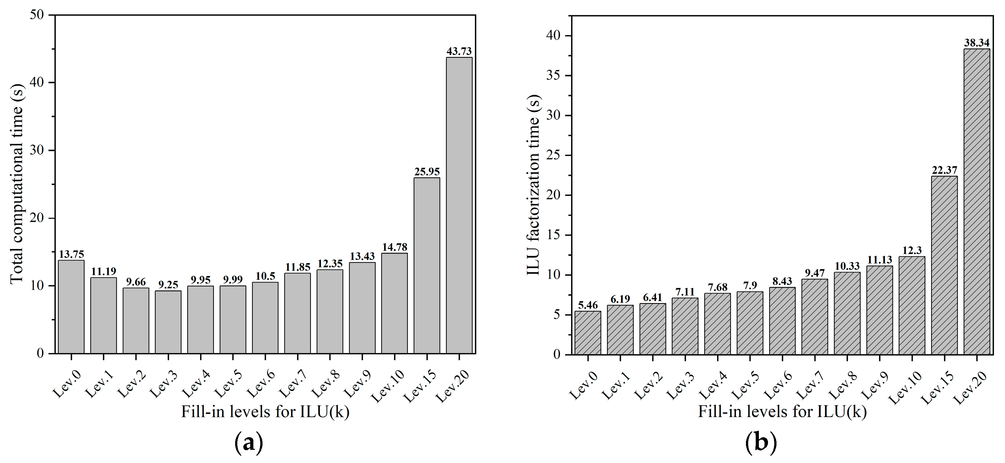
The total computational time and ILU factorization time with natural ordering for LRA problems under different fill-in levels are shown in Figure 8. Figure 9 shows total linear steps and non-zero elements under different fill-in levels. With an increase in the fill-in level, the number of linear steps required for calculation will decrease due to the faster convergence rate. Thus, the number of linear iteration steps is reduced. At the same time, as the fill-in level increases, the number of non-zero elements in the factorized matrix also increases, which means more computational complexity. This ultimately leads to a rise in the factorization time of the ILU(k) method, as shown in Figure 8. The factorization time of ILU(20) with original ordering is seven times that of ILU(0), indicating that the computational performance of the original natural ordering ILU(k) preconditioner is sensitive to the choice of fill-in level k. The ILU factorization process dominates the entire computational cost at high fill-in levels. Please note that, in practice, the user-defined fill-in level k is usually problem-dependent, which is not easy to determine.

In order to find a robust preconditioner, the key point is to make the preconditioner not sensitive to the user-defined fill-in level $k$. Therefore, it should reduce the computational cost of ILU(k) at the high fill-in levels. Here, the reordering algorithms are used for ILU(k) factorization, and the fill-in levels of $k=10$ are considered in this work. Compared with the ILU(10) under the natural ordering, the number of non-zeros after factorizations under reordering algorithms is reduced, as shown in

Table 3. Computing performance of different reordering algorithms in ILU(10).

	Natural	1WD	ND	QMD	RCM
Total computational time	34.996	30.609	29.756	31.193	29.871
Non-zeros after factorizations	3,884,202	2,442,293	1,879,544	2,337,351	1,919,274
Number of residual evaluations	556	556	556	556	556
Nonlinear steps	11	11	11	11	11
Linear steps	225	225	225	225	225

. Therefore, compared with the natural ordering, the total computational time of ILU(10) under reordering algorithms is relatively robust.

In order to further analyze the performance of the reordering-based ILU(k) preconditioner, a steady-state neutron diffusion k-eigenvalue problem with thermal-hydraulic feedback is also utilized as a supplement. It is a simplified 2D-PWR (Pressurized Water Reactor) reactor model, which includes the steady-state neutron diffusion k-eigenvalue equation as well as three other physical fields to consider the thermal-hydraulic feedback effect: coolant temperature, pressure, and velocity. As with most reactor systems, the neutronics and thermal hydraulics are tightly two-way coupled. The governing equations, coefficients, dimensions, and boundary conditions can be found in the reference paper [42,43]. As a simplified model, a $40\times 40$ cylindrical grid is used here. Here, the convergence criterion consistent with the previous example is used, and the SL coloring algorithm is used to generate the coefficient matrix automatically.

Figure 10 shows the results of the total computational time and the number of non-zero elements after factorization under different fill-in levels and reordering algorithms. The results of fill-in levels from 0 to 12 are provided, and the higher fill-in levels are redundant in practice for this multi-physics coupling problem. With the increase in fill-in level k, the factorization time of ILU(k) with natural ordering grows up significantly, as shown in Figure 10a, indicating it is sensitive to the choice of fill-in level k. Compared with the ILU factorization under natural ordering, the total computational time of ILU with reordering algorithms is not sensitive to the fill-in levels. Additionally, the computational performances are close to the optimal computational cost with natural ordering, as shown in Figure 10.

In detail,

Table 4. The optimal fill-in level and computational performance in different reordering algorithms.

	Natural	ND	RCM	1WD	QMD
Fill-in level $k$	3	11	8	7	11
Total computational time (s)	30.89	30.76	31.02	31.08	30.93
Factorization time (s)	23.26	26.35	24.33	24.26	26.52
Total nonlinear steps	6	3	4	4	3
Total linear steps	119	38	55	57	38

summarizes the results of different reordering algorithms under the optimal fill-in levels. The factorization times of low fill-in levels are relatively small, but more nonlinear/linear steps are required to achieve convergence. The reordering algorithms can reduce the cost of factorization at high fill-in levels. Although it is still time-consuming, it can improve efficiency by reducing the number of iteration steps. As a result, The performance of ILU(11) with the ND algorithm is slightly superior to ILU(3) with natural ordering. So, although natural ordering only could achieve good computational efficiency at low fill-in levels, such as $\mathrm{k}=3$, the computational time will increase sharply as the fill-in level increases. The superiority of reordering algorithms emerges in this situation. The reordering-based ILU preconditioner can adapt to a wide range of fill-in levels without empirical selection.

5. Conclusions

Efficient and robust preconditioners are a key issue to solve nonlinear problems in the nuclear engineering community, especially within the framework of the JFNK method. There are two important steps for the preconditioning matrix, constructing the preconditioner and its matrix factorization. For the first step, an efficient preconditioning-based coloring algorithm is developed in this work, which significantly reduces the cost of finite difference computation by partitioning the columns of the coefficient matrix. For the second step, the robust reordering-based ILU(k) preconditioner is developed, which could achieve a high computational performance for a wide range of fill-in levels. As a preliminary work, the 2D-LRA neutron eigenvalue problem and a simplified PWR model are provided to demonstrate the performance of the preconditioner. The results show that the proposed preconditioner can automatically generate the preconditioning matrix and has strong robustness. The main conclusions are:

• The finite difference technique combined with the coloring algorithm is utilized to automatically construct a preconditioning matrix, whose computational efficiency could be about 60 times higher than that without the coloring algorithm.
• With the increase in fill-in level k, the factorization time of ILU(k) with natural ordering grows up significantly, indicating its computational performance is relatively sensitive to the choice of fill-in level k, since the additional non-zero fill-in element increases rapidly.
• The reordering algorithms are utilized to reduce the non-zero fill-in element in ILU(k). The reordering-based ILU(k) algorithm is a robust preconditioning matrix factorization method. Moreover, its performance under different fill-in levels are comparable to the optimal computational cost with natural ordering.

The reordering-based ILU(k) factorization presented in this work exhibited good computational performance and robustness. In this work, the steady-state neutron diffusion k-eigenvalue problem was considered, which is the key part of the physics design of the nuclear reactor. Future work will focus on the performance of the proposed preconditioner for practical transient neutronic/thermal-hydraulic coupling problems, and to perform the nuclear reactor safety analysis.

References

- Wu, Y.; Liu, B.; Zhang, H.; Guo, J.; Li, F. A multi-level nonlinear elimination-based JFNK method for multi-scale multi-physics coupling problem in pebble-bed HTR. Ann. Nucl. Energy 2022, 176, 109281. [Google Scholar] [CrossRef]
- Novak, A.; Peterson, J.; Zou, L.; Andrš, D.; Slaybaugh; Martineau, R. Validation of Pronghorn friction-dominated porous media thermal-hydraulics model with the SANA experiments. Nucl. Eng. Des. 2019, 350, 182–194. [Google Scholar] [CrossRef]
- Benzi, M. Preconditioning Techniques for Large Linear Systems: A Survey. J. Comput. Phys. 2002, 182, 418–477. [Google Scholar] [CrossRef]
- Simon, Y.; David, R. Development and Testing of TRACE/PARCS ECI Capability for Modelling CANDU Reactors with Reactor Regulating System Response. Sci. Technol. Nucl. Install. 2022, 2022, 7500629. [Google Scholar]
- Li, S.; Liu, Z.; Chen, J.; Zhang, M.; Cao, L.; Wu, H. Development of high-fidelity neutronics/thermal-hydraulics coupling system for the hexagonal reactor cores based on NECP-X/CTF. Ann. Nucl. Energy 2023, 188, 109822. [Google Scholar] [CrossRef]
- Pinem, S.; Dibyo, S.; Luthfi, W.; Wardhani, V.I.S.; Hartanto, D. An Improved Steady-State and Transient Analysis of the RSG-GAS Reactor Core under RIA Conditions Using MTR-DYN and EUREKA-2/RR Codes. Sci. Technol. Nucl. Install. 2022, 2022, 6030504. [Google Scholar] [CrossRef]
- Wu, Y.; Liu, B.; Zhang, H.; Zhu, K.; Kong, B.; Guo, J.; Li, F. Accuracy and efficient solution of helical coiled once-through steam generator model using JFNK method. Ann. Nucl. Energy 2021, 159, 108290. [Google Scholar] [CrossRef]
- Fan, J.; Gou, J.; Huang, J.; Shan, J. A fully-implicit numerical algorithm of two-fluid two-phase flow model using Jacobian-free Newton–Krylov method. Int. J. Numer. Methods Fluids 2022, 95, 361–390. [Google Scholar] [CrossRef]
- Hu, G.; Zou, L.; O’Grady, D.J.; Hu, R. An integrated coupling model for solving multiscale fluid-fluid coupling problems in SAM code. Nucl. Eng. Des. 2023, 404, 112186. [Google Scholar] [CrossRef]
- Liu, L.; Wu, Y.; Liu, B.; Zhang, H.; Guo, J.; Li, F. A modified JFNK method for solving the fundamental eigenmode in k-eigenvalue problem. Ann. Nucl. Energy 2022, 167, 108823. [Google Scholar] [CrossRef]
- Ahmed, N.; Singh, S.; Kumar, N. Physics-based preconditioning of Jacobian-free Newton–Krylov solver for Navier–Stokes equations using nodal integral method. Int. J. Numer. Methods Fluids 2024, 96, 138–160. [Google Scholar] [CrossRef]
- Gaston, D.R.; Permann, C.J.; Peterson, J.W.; Slaughter, A.E.; Andrš, D.; Wang, Y.; Short, M.P.; Perez, D.M.; Tonks, M.R.; Ortensi, J.; et al. Physics-based multiscale coupling for full core nuclear reactor simulation. Ann. Nucl. Energy 2015, 84, 45–54. [Google Scholar] [CrossRef]
- Belcourt, N.; Pawlowski, R.P.; Schmidt, R.C.; Hooper, R.W. An Introduction to LIME 1.0 and Its Use in Coupling Codes for Multiphysics Simulations; Sandia National Laboratories: Albuquerque, NM, USA, 2011.
- Belcourt, N.; Bartlett, R.A.; Pawlowski, R.P.; Schmidt, R.C.; Hooper, R.W. A Theory Manual for Multi-Physics Code Coupling in LIME; Sandia National Laboratories: Albuquerque, NM, USA, 2011.
- DeHart, M.; Gleicher, F.; Harter, J.; Labour, V.; Ortensi, J.; Schunert, S.; Wan, Y. MAMMOTH Theory Manual; Technical Report INL/EXT-19-54252; Idaho National Laboratory: Idaho Falls, ID, USA, 2019.
- Lee, J.; Balestra, P.; Hassan, Y.A.; Muyshondt, R.; Nguyen, D.T.; Skifton, R. Validation of Pronghorn Pressure Drop Correlations Against Pebble Bed Experiments. Nucl. Technol. 2022, 208, 1769–1805. [Google Scholar] [CrossRef]
- Andrs, D.; Berry, R.; Gaston, D.; Martineau, R.; Peterson, J.; Zhang, H.; Zhao, H.; Zou, L. RELAP-7 Level 2 Milestone Report: Demonstration of a Steady State Single Phase PWR Simulation with RELAP-7; Technical Report; Idaho National Lab. (INL): Idaho Falls, ID, USA, 2012.
- Liu, Z.; Xu, X.; Wu, H.; Cao, L. Multidimensional multi-physics simulations of the supercritical water-cooled fuel rod behaviors based on a new fuel performance code developed on the MOOSE platform. Nucl. Eng. Des. 2021, 375, 111085. [Google Scholar] [CrossRef]
- Hales, J.; Novascone, S.; Spencer, B.; Williamson, R.; Pastore, G.; Perez, D. Verification of the BISON fuel performance code. Ann. Nucl. Energy 2014, 71, 81–90. [Google Scholar] [CrossRef]
- Lin, C.J.; More, J.J. Incomplete Cholesky factorizations with limited memory. SIAM J. Sci. Comput. 1999, 21, 24. [Google Scholar] [CrossRef]
- Cuthill, E.; Mckee, J. Reducing the bandwidth of sparse symmetric matrices. In Proceedings of the 24th National Conference ACM 1969, New York, NY, USA, 26–28 August 1969; pp. 157–172. [Google Scholar]
- Benchmark Problem Book, ANL-7416-Suppl. 2; Argonne National Laboratory: Lemont, IL, USA, 1979.
- Executioner for Eigenvalue Problems. INL. Available online: https://mooseframework.inl.gov/source/executioners/NonlinearEigen.html (accessed on 1 October 2022).
- Zhang, H.; Guo, J.; Li, F.; Xu, Y.; Downar, T. Efficient simultaneous solution of multi-physics multi-scale nonlinear coupled system in HTR reactor based on nonlinear elimination method. Ann. Nucl. Energy 2018, 114, 301–310. [Google Scholar] [CrossRef]
- Greenbaum, A.; Pták, V.; Strakoš, Z.E.K. Any Nonincreasing Convergence Curve is Possible for GMRES. SIAM J. Matrix Anal. Appl. 1996, 17, 465–469. [Google Scholar] [CrossRef]
- Saad, Y. Iterative Methods for Sparse Linear Systems; PWS Publishing: Boston, MA, USA, 1996. [Google Scholar]
- Bruun, A. Direct Methods for Sparse Matrices. Math. Comput. 1980, 9, 874. [Google Scholar]
- Hossain, A.K.M.S.; Steihaug, T. Computing a Sparse Jacobian Matrix by Rows and Columns. Optim. Methods Softw. 1998, 10, 33–48. [Google Scholar] [CrossRef]
- Hovland, P.D. Combinatorial problems in automatic differentiation. In Proceedings of the SIAM Workshop on Combinatorial Scientific Computing, San Fransisco, CA, USA, 28 February 2004. [Google Scholar]
- Bondy, J. Bounds for the chromatic number of a graph. J. Comb. Theory 1969, 7, 96–98. [Google Scholar] [CrossRef]
- Brooks, R.L. On coloring the nodes of a network. Proc. Camb. Philos. Soc. 1941, 37, 194–197. [Google Scholar] [CrossRef]
- Welsh, D.J.A.; Powell, M.B. An upper bound for the chromatic number of a graph and its application to timetabling problems. Comput. J. 1967, 10, 85–86. [Google Scholar] [CrossRef]
- Coleman, T.F.; Moré, J.J. Estimation of Sparse Jacobian Matrices and Graph Coloring Problems. SIAM J. Numer. Anal. 1983, 20, 187–209. [Google Scholar] [CrossRef]
- Matula, D.W.; Marble, G.; Isaacson, J.D. Graph Coloring Algorithms. In Graph Theory and Computing; Academic Press: Cambridge, MA, USA, 1972; pp. 109–122. [Google Scholar]
- Bozdağ, D.; Catalyurek, U.; Gebremedhin, A.H.; Manne, F.; Boman, E.G.; Özgüner, F. A parallel distance-2 graph coloring algorithm for distributed memory computers. In Proceedings of the International Conference on High Performance Computing & Communications, Sorrento, Italy, 21–23 September 2005; Springer: Berlin/Heidelberg, Germany, 2005. [Google Scholar]
- Iii, W.; James, W. A Conjugate Gradient-Truncated Direct Method for the Iterative Solution of the Reservoir Simulation Pressure Equation. Soc. Pet. Eng. J. 1981, 21, 345–353. [Google Scholar]
- Saad, Y. Finding Exact and Approximate Block Structures for ILU Preconditioning. SIAM J. Sci. Comput. 2003, 24, 1107–1123. [Google Scholar] [CrossRef]
- Gustafsson, I. A class of first order factorization methods. BIT Numer. Math. 1978, 18, 142–156. [Google Scholar] [CrossRef]
- Saad, Y. ILUT: A dual threshold incomplete LU factorization. Numer. Linear Algebra Appl. 1994, 1, 387–402. [Google Scholar] [CrossRef]
- Bolstad, J.H.; Leaf, G.K.; Lindeman, A.J.; Kaper, H.G. An Empirical Investigation of Reordering and Data Management for Finite Element Systems of Equations; Rep. ANL-8056; Argonne National Laboratory: Lemont, IL, USA, 1973.
- Davis, T.A.; Gilbert, J.R.; Larimore, S.I.; Ng, E.G. A column approximate minimum degree ordering algorithm. ACM Trans. Math. Softw. 2004, 30, 353–376. [Google Scholar] [CrossRef]
- Liu, L.; Zhang, H.; Wu, Y.; Liu, B.; Guo, J.; Li, F. A modified JFNK with line search method for solving k-eigenvalue neutronics problems with thermal-hydraulics feedback. Nucl. Eng. Technol. 2023, 55, 310–323. [Google Scholar] [CrossRef]
- Zhang, H.; Guo, J.; Lu, J.; Niu, J.; Li, F.; Xu, Y. The comparison between nonlinear and linear preconditioning JFNK method for transient neutronics/thermal-hydraulics coupling problem. Ann. Nucl. Energy 2019, 132, 357–368. [Google Scholar] [CrossRef]
Figure 1.
Schematic of LRA benchmark, (1) fuel 1 with rod, (2) fuel 1 without rod, (3) fuel 2 with rod, (4) fuel 2 without rod, (5) reflector.
Figure 2.
Preconditioning system in MOOSE.
Figure 3.
Preconditioning matrix and its compressed representation in steady-state neutron diffusion problem. (The color dots represent non-zero matrix elements, and each color represents a structurally orthogonal group) (a) Preconditioning matrix; (b) Its compressed representation.
Figure 4.
Sparse matrix and its corresponding graph. (a) Sparse matrix; (b) Corresponding graph with degrees.
Figure 5.
Matrix columns partitioned based on largest-first ordering. (a) Columns rearrangement in matrix form based on LF ordering; (b) Compressed matrix generation based on LF ordering; (c) Columns rearrangement in graph form based on LF ordering.
Figure 6.
Matrix structure of different reordering methods using ILU(20).
Figure 7.
Residual history in three coloring methods using FDP.
Figure 8.
The total computational time and factorization time in ILU(k) algorithm. (a) Computational time; (b) Factorization time.
Figure 9.
The linear steps and non-zeros after ILU factorization. (a) Total linear steps; (b) Number of non-zeros.
Figure 10.
The total computational time and non-zeros of ILU factorization for simplified PWR model. (a) Total computational time; (b) Number of non-zeros.