Energy Efficiency Assessment and Prediction Based on Indicator System, PSO + AHP − FCE Model and Regression Algorithm

Abstract

Energy-intensive enterprises lack a scientific and effective energy efficiency assessment framework and methodology. This lack leads to an inaccurate understanding of energy usage and its benefits. As a result, there is energy wastage and loss. This wastage and loss negatively affect product costs. They also present a challenge to effective energy management. To address these issues, this paper introduces a novel, comprehensive energy efficiency evaluation system. This system integrates both qualitative and quantitative measures. It proposes an evaluation model based on the Particle Swarm Optimization (PSO) combined with the Analytic Hierarchy Process (AHP) and Fuzzy Comprehensive Evaluation (FCE), wherein PSO is employed to optimize the weights determined by AHP, ensuring that the significance attributed to various indicators is scientific, objective, and rational. The FCE method is utilized to convert diverse factors affecting corporate energy efficiency, across different types and scales, into standardized 0–1 values, enabling a comparative analysis of the impact of each process and indicator on energy efficiency. Furthermore, the paper introduces an energy efficiency prediction model employing a multivariate linear regression algorithm, which demonstrates a good fit, facilitating the transition from retrospective energy efficiency evaluation to proactive improvements. Utilizing data on actual consumption of water, electricity, and steam from an enterprise, along with expert assessments on the implementation levels of new processes, technologies, equipment, personnel scheduling proficiency, steam recovery rates, and adherence to policies and assessments, a simulation experiment of the proposed model was conducted using Python. The evaluation yielded an energy efficiency score of 0.68; this is consistent with the real-world scenario of the studied enterprise. The predicted mean square error of 9.035416039503998 $\times {10}^{-9}$ indicates a high model accuracy, validating the practical applicability and effectiveness of the proposed approach.

1. Introduction

Many current evaluations of corporate energy efficiency focus primarily on direct energy consumption, mainly reflecting energy use through a company’s physical infrastructure. This approach often overlooks comprehensive assessments that include process enhancements, equipment upgrades, recycling initiatives, and adherence to policies and regulatory frameworks; areas where a gap is evident compared to international energy efficiency standards.

In the brewing industry, beer production enterprises are significant consumers of energy and major sources of pollution and waste discharge. The specific process of beer manufacturing involves several steps: milling, followed by mashing and saccharification; then wort filtration; boiling with hops at high temperatures; clarification and cooling; addition of yeast for fermentation; diatomaceous earth filtration; and finally packaging of the finished product. This process encompasses various departments, including the power workshop, brewing workshop, and packaging workshop. This cycle encompasses various facilities, including power generation, brewing operations, and packaging. By prioritizing energy management and optimizing the use of water, electricity, and steam, breweries can ensure product quality and achieve significant economic and environmental benefits. Establishing an energy efficiency assessment indicator system and evaluation model is key and of great significance [1,2,3].

Paper [1] utilizes PSO + AHP and FCE to assess the operational status of wind power systems. In paper [2], it is indicated that a method for corporate energy consumption process modeling provides a multi-dimensional model and an open integration framework for enterprise energy consumption systems, alongside methods for simulating and optimizing energy consumption processes and analyzing energy flow and logistics balance within enterprise production processes. This focuses on sub-models of the enterprise energy consumption system and methods for simulating and optimizing energy consumption processes. However, it does not involve the evaluation of energy efficiency. Paper [3] employs a fuzzy comprehensive assessment method for evaluating the health status of hoists. Article [4] employs self-coding compression and multi-scale feature extraction for predicting the degradation assessment of pumped storage units.

Furthermore, paper [5] reviews the use of data envelopment analysis (DEA) for energy efficiency evaluation, showcasing DEA as a data-oriented method for estimating the overall efficiency of homogeneous decision-making units based on input–output ratios. In paper [6], it is indicated that the basic models, development, and application of four main assessment methods in energy efficiency evaluation, including stochastic frontier analysis, data envelopment analysis, power analysis, and benchmarking comparison. References [5,6] merely involve objective energy consumption data and do not cover the soft environment of enterprises, such as the application of new processes, new technologies, and new equipment, the scheduling level of professionals, the recovery rate of water vapor, and other subjective factors. Article [7] utilizes the primary energy input–output (PEIO) ratio as an assessment method to evaluate the energy balance of a biogas system. Article [8] proposes a mathematical model based on the target cost approach for selecting energy efficiency projects aimed at maximizing economic impacts.

Paper [9] emphasizes the need for targeted interventions based on industry characteristics and the responsibility of various sectors in promoting energy efficiency. It calls for the adoption of comprehensive methods to integrate energy-saving standards into product production. This further underscores the significance and societal value of this article, highlighting it as a subject that requires focused and in-depth research in the field of energy. In paper [10], a method for assessing the energy efficiency of industrial equipment based on informational means is described. Reference [11] established a comprehensive energy efficiency indicator framework for high-energy-consuming enterprises, encompassing economic, management, technical energy efficiency indicators, and environmental indicators. However, it does not provide methods for measuring each indicator. In article [12] an index system has been established for electric companies, encompassing economic energy efficiency indicators, electrical energy information indicators, production information indicators, and electrical energy pollution indicators. However, the subjective weights derived from G1 group judgments have not undergone consistency assessment. In article [13] the corporate energy efficiency is evaluated based on the Analytic Hierarchy Process (AHP) and quantitative specific consumption data. Paper [14] gives a comprehensive evaluation of the smart power distribution network’s effectiveness, including reliability, electrical energy quality, economy, environmental protection, interactivity, and technicality, established based on AHP, entropy weighting method, and fuzzy comprehensive analysis. Paper [15], through theoretical calculation and combining actual sintering production practices, studies and establishes a standardized sintering process energy efficiency assessment system. Article [16] gives a comprehensive energy efficiency assessment framework for medium- and low-voltage distribution networks, as well as primary thermal networks. This has been developed and evaluated using the Analytic Hierarchy Process (AHP). Article [17] combines subjective and objective weights obtained from Particle Swarm Optimization Analytic Hierarchy Process (PSO-AHP) and Rough Set Theory based on the idea of linear weighting to acquire combined weights, and uses a Fuzzy Comprehensive Evaluation method to assess the efficiency of irrigation water use. Paper [18] uses AHP to establish a hierarchical progressive analysis model, and through the simulated annealing method improves the Particle Swarm Optimization method to solve the consistency problem of judgment matrices, addressing the issues of strong subjectivity and uncertainty in information security threat assessments. Paper [19], considering distributed power sources and combined with reclosure devices, proposes a new method that improves Particle Swarm Optimization and Analytic Hierarchy Process to simultaneously optimize the capacity, location, and quantity. Paper [20], based on the Particle Swarm Optimization Algorithm (PSO), constructs the PSO-AHP model, applying this model to evaluate the impact of the water transport industry on the new rural construction in Nanjing’s Wu Jiazui Village; Article [21] uses the AHP-FCE method combined with expert questionnaire results and Fuzzy Comprehensive Evaluation to calculate weights at all levels, scientifically evaluating factors affecting quality in the commercial concrete production process, thereby enhancing the management efficiency of commercial concrete operations. Paper [22] constructis an agricultural product supply chain performance evaluation indicator system, using the AHP-FCE model as the evaluation method. In paper [23], Analytic Hierarchy Process (AHP)—Fuzzy Comprehensive Evaluation (FCE) mathematical model is adopted to establish a comprehensive evaluation system for 20 Macadamia germplasm resources, and then combines the Technique for Order Preference by Similarity to Ideal Solution (TOPSIS) to screen for Macadamia strains with superior comprehensive trait performance. Article [24] constructs a pharmaceutical wastewater treatment technology evaluation index system, sets evaluation standards, and uses the Analytic Hierarchy Process combined with Fuzzy Comprehensive Evaluation (AHP-FCE) to conduct a comprehensive evaluation of 13 pharmaceutical wastewater treatment technologies developed for a water-specific project. Article [25] proposes a comprehensive performance evaluation method for electromagnetic coupling mechanisms, evaluating various types of electromagnetic coupling mechanisms that meet the same application requirements.

Building on the foundation of the aforementioned literature, the aim of this study is to conduct an energy efficiency assessment for enterprises. For the first time, an enterprise energy efficiency assessment indicator system has been developed, which not only considers real-time objective data (such as water, electricity, and steam consumption) but also takes into account subjective evaluations of new technologies and equipment, professional personnel arrangements, water vapor recovery rate, and the status of regulations and assessment implementation. A quantitative evaluation model combining Particle Swarm Optimization + Analytic Hierarchy Process − Fuzzy Comprehensive Evaluation (PSO + AHP − FCE) is proposed to assess enterprise energy efficiency, identify weaknesses affecting energy efficiency, and facilitate targeted rectification. Moreover, based on the assessment results, a multivariate linear regression method for energy efficiency prediction is put forward, shifting from post-assessment to pre-estimation, retracing factors leading to low energy efficiency, and guiding enterprises in specifically improving relevant technologies and optimizing production scheduling, etc., to enhance energy efficiency. This analytical and optimization approach provides a means to accurately grasp the trend of corporate energy efficiency, promote scientific production scheduling, and achieve energy saving, cost reduction, and efficiency improvement. This method is designed to accurately capture the trend of corporate energy efficiency, facilitate scientific production scheduling, and realize energy conservation, cost reduction, and efficiency enhancement.

2. Principles to Be Followed in Constructing the Energy Efficiency Assessment Index System

In evaluating the energy efficiency of breweries within the brewing sector, it is essential to apply a range of indicators that accurately reflect their energy performance. The selection of these indicators must adhere to specific criteria to ensure a comprehensive representation of a brewery’s energy efficiency [10,11].

Precision: The foundation and selection of the assessment framework, including indicators and methodologies, must be precise to produce reliable assessment outcomes. This precision ensures that the chosen indicators are clear and minimizes their interdependence, to uphold the authenticity and trustworthiness of the results.

Inclusiveness: The chosen indicators should offer an holistic view of the brewery’s energy consumption and efficiency, spanning various aspects such as water, electricity, and steam usage across different processes.

Applicability and Universality: Indicators should conform to universally accepted measurement conventions, incorporating both objective and measurable data and, where feasible, subjective assessments that are straightforward to gauge.

Organized and Structured Approach: There should be a clear, logical flow from overarching energy efficiency goals down to specific factors impacting these goals, establishing a coherent structure among the indicators.

Integrated Approach: It is essential to balance both quantitative and qualitative indicators. Quantitative indicators should capture the core aspects of energy efficiency. In contrast, though more challenging to measure, qualitative indicators can be quantified based on expert evaluations to encompass elements critical to understanding the brewery’s energy efficiency landscape.

3. Construction of Energy Efficiency Evaluation System

In assessing the energy efficiency of beer enterprises, this study compares and analyzes the technologies and equipment adopted in various production stages, the processes involved in production, and the competencies of technical and management personnel. Beyond relying solely on quantifiable metrics such as water, electricity, and steam consumption to gauge enterprise energy efficiency, this research integrates both qualitative and quantitative assessments. It incorporates into the comprehensive energy efficiency evaluation indices those aspects that cannot be directly measured, such as the application of new processes, technologies, and equipment, the scheduling proficiency of professional personnel, the rate of water and steam recovery and reuse, and the energy management systems and evaluations, which are only amenable to qualitative assessment. This approach enables the measurement of the soft environment management level within different subsidiaries of the group, under the fixed conditions of hardware equipment, in terms of different process modifications, technological innovations, professional personnel scheduling, and management of leaks and losses.

Each type of energy consumption, such as electricity consumption, is determined by different stages of consumption, including brewing electricity consumption, power electricity consumption, packaging electricity consumption, and non-production electricity consumption. Among these, various process stages such as saccharification, fermentation, filtration, and CIP cleaning further determine brewing electricity consumption. This reflects the systemic nature of the enterprise, where energy consumption and its hierarchically related indicators are interlinked.

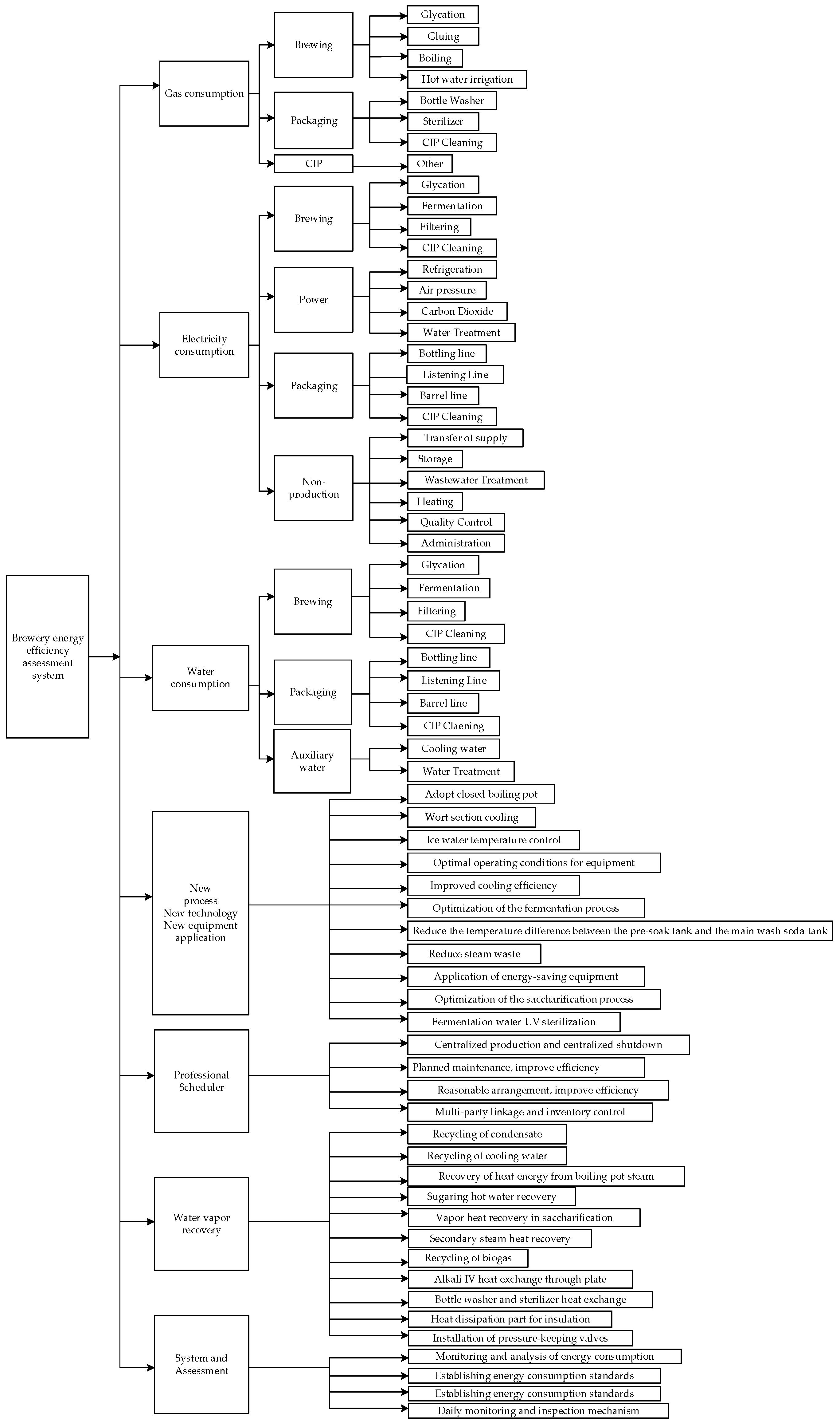
For instance, the application of new processes, technologies, and equipment involves 11 secondary indicators, as shown in Figure 1; water and steam recovery rates involve 11 secondary indicators; the level of professional staff scheduling involves four secondary indicators; the implementation of systems and assessments involves four secondary indicators; electricity consumption involves four secondary indicators for brewing, power, packaging, and non-production, with brewing electricity consumption further involving four tertiary indicators such as saccharification, fermentation, filtration, and CIP cleaning, etc. The energy efficiency assessment indicator system constructed is shown in Figure 1.

This section proposes incorporating four qualitative aspects alongside seven quantifiable primary indicators into the comprehensive energy efficiency assessment framework. These aspects include the application of new processes, technologies, and equipment; the level of professional personnel scheduling; water and steam recovery rates; and the implementation of systems and assessments—all of which significantly impact energy efficiency levels but are not directly measurable. The goal layer of the assessment index includes these alongside measurable consumptions of water, electricity, and steam.

The criterion layer encompasses the various stages affecting related factors and the methods adopted. It includes specific consumption metrics such as brewing steam, packaging steam, CIP (Clean-In-Place) steam, brewing electricity, power electricity, packaging electricity, non-production electricity, brewing water, packaging water, auxiliary water usage, and the application of energy-efficient technologies and practices. Among these are the use of enclosed boiling kettles, optimization of saccharification processes, wort cooling, ice water temperature control, fermentation process optimization, optimal equipment operating conditions, reduction of steam waste, minimizing temperature differences in pre-soaking and main caustic tanks, using energy-saving devices, UV sterilization for fermentation water, improving refrigeration efficiency, centralized production and cessation, planned maintenance for efficiency enhancement, reasonable scheduling for benefit improvement, multi-party linkage to control inventory, recovery and reuse of condensate water, circulation of cooling water, recovery of steam heat energy from malt boiling, saccharification hot water recovery, steam heat energy recovery in saccharification, secondary steam heat recovery, biogas recovery and utilization, alkali recovery through plate heat exchange, heat exchange between bottle washers and sterilizers, insulation of heat dissipation areas, installation of pressure-maintaining valves, energy consumption monitoring and analysis, setting energy consumption standards, establishing an energy assessment mechanism, and mechanisms for daily supervision and inspection; totaling 40 secondary indicators.

Within the criterion layer, various processes are included as the indicator layer, such as steam consumption for brewing saccharification, gelatinization, boiling, hot water tanks, bottle washing machines, sterilizers, CIP cleaning, and electricity consumption for power refrigeration, air compression, carbon dioxide production, water treatment, bottling lines, canning lines, kegging lines, non-production transfer, storage, sewage treatment, heating, process control, administrative activities, and water consumption for brewing saccharification, fermentation, filtration, CIP cleaning, and auxiliary uses; totaling 36 tertiary indicators.

For quantifiable objective indicators, their weights are determined by their importance at the corresponding level. For instance, in beer production enterprises, the proportion of steam consumption is the highest, hence its weight is the greatest; while the proportion of water consumption is the lowest, making its weight the smallest. As for unquantifiable subjective indicators, through in-depth research and analysis conducted jointly with process and technology experts and onsite engineering technicians, the ranking of factors affecting enterprise energy efficiency has been determined as follows: the application of new processes, technologies, and equipment; the level of professional personnel scheduling; the rate of steam recovery; and the implementation of policies and assessments.

The specific factors influencing energy efficiency and the order of their weights are shown in Figure 1 and Equations (1) to (18).

As can be seen in Figure 1, the set of weights of the first level indicators and the ranking of the weights:

$$\begin{gathered} U=\left\{U_1,U_2,U_3,U_4,U_5,U_6,U_7,U_8,U_9\right\} \\ {\omega }_1>{\omega }_4>{\omega }_2>{\omega }_5>{\omega }_6>{\omega }_3>{\omega }_7 \end{gathered}$$

(1)

Set of weights for secondary indicator steam consumption:

$$\begin{gathered} U_1=\left\{U_{11},U_{12},U_{13}\right\} \\ {\omega }_{12}>{\omega }_{11}>{\omega }_{13} \end{gathered}$$

(2)

Set of weights for secondary indicator electricity consumption:

$$\begin{gathered} U_2=\left\{U_{21},U_{22},U_{23},U_{24}\right\} \\ {\omega }_{22}>{\omega }_{23}>{\omega }_{24}>{\omega }_{21} \end{gathered}$$

(3)

Set of weights for secondary indicator water consumption:

$$\begin{gathered} U_3=\left\{U_{31},U_{32},U_{33}\right\} \\ {\omega }_{31}>{\omega }_{32}>{\omega }_{33} \end{gathered}$$

(4)

Set of weights for secondary indicator application of new processes, technologies, and equipment:

$$\begin{gathered} U_4=\left\{U_{41},U_{42},U_{43},U_{44},U_{45},U_{46},U_{47},U_{48},U_{49},U_{410},U_{411}\right\} \\ {\omega }_{41}>{\omega }_{42}>{\omega }_{43}>{\omega }_{44}>{\omega }_{45}>{\omega }_{46}>{\omega }_{47}>{\omega }_{48}>{\omega }_{49}>{\omega }_{410}>{\omega }_{411} \end{gathered}$$

(5)

Set of weights for secondary indicator professional scheduling:

$$\begin{gathered} U_5=\left\{U_{51},U_{52},U_{53},U_{54}\right\} \\ {\omega }_{51}>{\omega }_{52}>{\omega }_{53}>{\omega }_{54} \end{gathered}$$

(6)

Set of weights for secondary indicator water vapor recovery and utilization:

$$\begin{gathered} U_6=\left\{U_{61},U_{62},U_{63},U_{64},U_{65},U_{66},U_{67},U_{68},U_{69},U_{610},U_{611}\right\} \\ {\omega }_{61}>{\omega }_{62}>{\omega }_{63}>{\omega }_{64}>{\omega }_{65}>{\omega }_{66}>{\omega }_{67}>{\omega }_{68}>{\omega }_{69}>{\omega }_{610}>{\omega }_{611} \end{gathered}$$

(7)

Set of weights for secondary indicator system assessment:

$$\begin{gathered} U_7=\left\{U_{71},U_{72},U_{73},U_{74}\right\} \\ {\omega }_{71}>{\omega }_{72}>{\omega }_{73}>{\omega }_{74} \end{gathered}$$

(8)

Set of weights for tertiary indicator brewing steam consumption:

$$\begin{gathered} U_{11}=\left\{U_{111},U_{112},U_{113},U_{114}\right\} \\ {\omega }_{113}>{\omega }_{11}>{\omega }_{112}>{\omega }_{114} \end{gathered}$$

(9)

Set of weights for tertiary indicator packaging steam consumption:

$$\begin{gathered} U_{12}=\left\{U_{121},U_{122},U_{123}\right\} \\ {\omega }_{121}>{\omega }_{122}>{\omega }_{123} \end{gathered}$$

(10)

Set of weights for tertiary indicator CPI (cost per unit) steam consumption:

$$\begin{gathered} U_{13}=\left\{U_{131}\right\} \\ {\omega }_{131}=1 \end{gathered}$$

(11)

Set of weights for tertiary indicator brewing electricity consumption:

$$\begin{gathered} U_{21}=\left\{U_{211},U_{212},U_{213},U_{214}\right\} \\ {\omega }_{211}>{\omega }_{212}>{\omega }_{213}>{\omega }_{214} \end{gathered}$$

(12)

Set of weights for tertiary indicator power electricity consumption:

$$\begin{gathered} U_{22}=\left\{U_{221},U_{222},U_{223},U_{224}\right\} \\ {\omega }_{221}>{\omega }_{222}>{\omega }_{223}>{\omega }_{224} \end{gathered}$$

(13)

Set of weights for tertiary indicator packaging electricity consumption:

$$\begin{gathered} U_{23}=\left\{U_{231},U_{232},U_{233},U_{234}\right\} \\ {\omega }_{231}>{\omega }_{232}>{\omega }_{233}>{\omega }_{234} \end{gathered}$$

(14)

Set of weights for tertiary indicator CPI (cost per unit) electricity consumption:

$$\begin{gathered} U_{24}=\left\{U_{241},U_{242},U_{243},U_{244},U_{245},U_{246}\right\} \\ {\omega }_{243}>{\omega }_{241}>{\omega }_{242}>{\omega }_{246}>{\omega }_{244}>{\omega }_{245} \end{gathered}$$

(15)

Set of weights for tertiary indicator brewing water consumption:

$$\begin{gathered} U_{31}=\left\{U_{311},U_{312},U_{313},U_{314}\right\} \\ {\omega }_{311}>{\omega }_{313}>{\omega }_{312}>{\omega }_{314} \end{gathered}$$

(16)

Set of weights for tertiary indicator packaging water consumption:

$$\begin{gathered} U_{32}=\left\{U_{321},U_{322},U_{323},U_{324}\right\} \\ {\omega }_{321}>{\omega }_{322}>{\omega }_{323}>{\omega }_{324} \end{gathered}$$

(17)

Set of weights for tertiary indicator auxiliary water consumption:

$$\begin{gathered} U_{33}=\left\{U_{331},U_{332}\right\} \\ {\omega }_{331}>{\omega }_{332} \end{gathered}$$

(18)

The subjective scoring is provided by a panel of five experts, consisting of hired group managers, corporate process specialists, vice presidents of technology, corporate energy monitoring technicians, and university researchers. This scoring arises from a collective process of comparison, analysis, and discussion by the panel, based on fundamental principles (non-adoption is scored as 0, adoption for half a year scores 50, and a score of about 0.85 is given for the inability to concentrate production or cease operations during the February Spring Festival and the November off-season, or for seasonal transitions). Given the consistency in scoring principles, the variance among individual scores is minimal. The scores, after being averaged arithmetically, are presented in

Table 1. Scores of indicators at each level.

Index	Numerical Value	Index	Numerical Value	Index	Numerical Value
$U_1$	0.201 T/kl	$U_2$	39.05 kwh/kl	$U_3$	2.3 T/kl
$U_4$	68.4	$U_5$	81.5	$U_6$	92.6
$U_7$	99.2	$U_{11}$	0.041 T/kl	$U_{12}$	0.099 T/kl
$U_{13}$	0.002 T/kl	$U_{21}$	3.56 kwh/kl	$U_{22}$	18.6 kwh/kl
$U_{23}$	19.7 kwh/kl	$U_{24}$	4.48 kwh/kl	$U_{31}$	1.56 T/kl
$U_{32}$	0.89 T/kl	$U_{33}$	0.065 T/kl	$U_{41}$	100
$U_{42}$	0	$U_{43}$	50	$U_{44}$	50
$U_{45}$	90	$U_{46}$	50	$U_{47}$	50
$U_{48}$	100	$U_{49}$	80	$U_{410}$	100
$U_{411}$	100	$U_{51}$	83	$U_{52}$	80
$U_{53}$	80	$U_{54}$	83	$U_{61}$	98
$U_{62}$	100	$U_{63}$	95	$U_{64}$	90
$U_{65}$	0	$U_{66}$	100	$U_{67}$	100
$U_{68}$	100	$U_{69}$	100	$U_{610}$	98
$U_{611}$	100	$U_{71}$	98	$U_{72}$	100
$U_{73}$	100	$U_{74}$	100	$U_{111}$	object
$U_{112}$	object	$U_{113}$	object	$U_{114}$	object
$U_{121}$	object	$U_{122}$	object	$U_{123}$	object
$U_{131}$	object	$U_{211}$	object	$U_{212}$	object
$U_{213}$	object	$U_{214}$	object	$U_{221}$	object
$U_{222}$	object	$U_{223}$	object	$U_{224}$	object
$U_{231}$	object	$U_{232}$	object	$U_{233}$	object
$U_{234}$	object	$U_{241}$	object	$U_{242}$
$U_{243}$	object	$U_{244}$	object	$U_{245}$
$U_{246}$	object	$U_{311}$	object	$U_{312}$
$U_{313}$	object	$U_{314}$	object	$U_{321}$
$U_{322}$	object	$U_{323}$	object	$U_{324}$
$U_{331}$	object	$U_{332}$	object

, as indicated. This translation is intended for an academic paper; therefore, terminology has been selected for precision and formality.

As shown in Table 1, enterprises considering food safety risks did not adopt wort cooling in the first stage, resulting in a score of $U_{42}$ being 0. When water temperatures are low during autumn and winter, reducing the refrigeration consumption for ice-making is feasible, with a score of $U_{43}$ being 0.5. The use of syrup, not employing the optimal operating conditions of the gelatinization pot, has a score of $U_{44}$ being 0.5. Optimizing fermentation processes, which are affected by seasonal variations, is only applicable for half of the year, leading to a score of $U_{46}$ being 0.5. Improving microbial management levels to reduce steam consumption, which is also limited by seasonality to half-year applicability, results in a score of $U_{47}$ being 0.5. These factors influence the score for the application of new processes, technologies, and equipment.

Extended downtime in February and November impacts the ability to concentrate production and cessation activities, scoring $U_{51}$ at 0.83. The transition from off-peak to peak seasons or vice versa affects multi-party coordination and the inventory of fermentation liquid, scoring $U_{54}$ at 0.83, which influences the scores for professional staff scheduling.

Although the recovery of evaporative steam heat during saccharification and gelatinization requires capital investment for equipment modification, it is scored $U_{65}$ at 0, indicating that its weight is minimal and does not significantly impact the water and steam recovery score.

The enterprise focuses on controlling issues such as constant lighting and leaking faucets, ensuring that energy management systems and assessments are effectively implemented, resulting in high scores.

Objective indicator values are collected by sensors daily, weekly, monthly, or annually, with data varying across different periods. This academic paper emphasizes the importance of precision in language to reflect the rigorous nature of the analysis.

4. Comprehensive Energy Efficiency Evaluation Model

To conduct a comprehensive, integrated, scientific, and objective evaluation of energy efficiency, it is necessary to understand the quantitative evaluation values; i.e., the magnitude of the weights, based on a qualitative foundation that ranks the importance of each indicator’s impact on energy efficiency (from Equation (1) to Equation (18)). Here, the subjective weighting method, the Analytic Hierarchy Process (AHP) model, determines the weights. Furthermore, these weights obtained from the AHP method are further optimized through the Particle Swarm Optimization (PSO) method to make them more objective and reasonable. This approach ensures a rigorous academic discourse on energy efficiency evaluation.

4.1. AHP Model

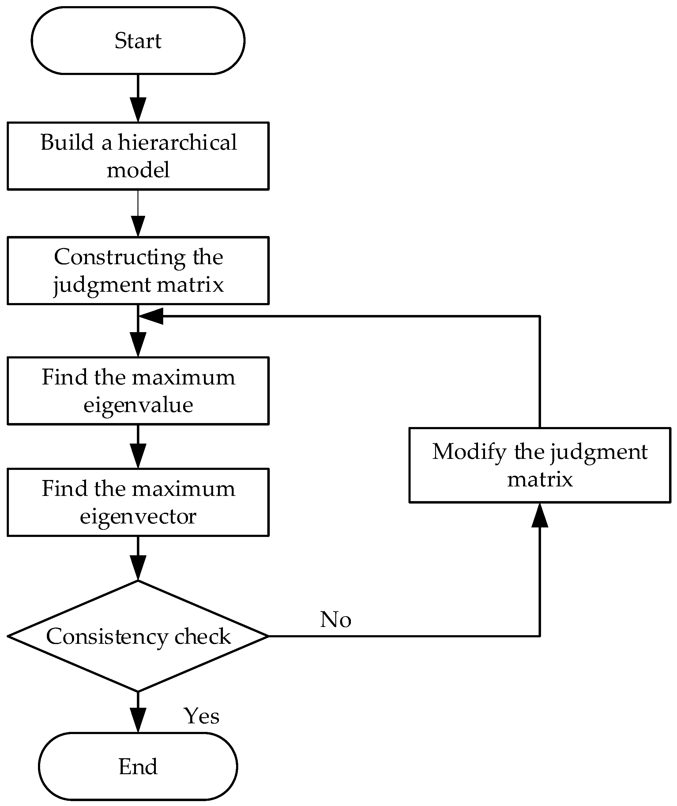
The Analytic Hierarchy Process (AHP) establishes a hierarchical structure model. The essence of AHP is to hierarchize and quantify the factors affecting energy efficiency. For this purpose, the complex, multi-dimensional issues affecting enterprise energy efficiency—encompassing various energy sources, different stages, and diverse factors—are decomposed from difficult to easy into corresponding primary, secondary, and tertiary indicators, as shown in Figure 1. Among the seven primary indicators, 40 secondary indicators, and 36 tertiary indicators of energy efficiency assessment, the evaluation of the application of new processes, technologies, and equipment, professional staff scheduling, water and steam recovery, and systems and assessments as primary indicators differs from the three primary objective indicators of steam, electricity, and water consumption. The subjective factors of different experts are inevitably prone to certain biases, which may lead to contradictions, resulting in the judgment matrix not being entirely consistent. Therefore, a consistency test is necessary to determine the importance of ranking the evaluation of the above indicators. Based on this, a qualitative and quantitative decision analysis is conducted. The process flow of the AHP application is illustrated in Figure 2.

After establishing the multi-level energy efficiency evaluation system shown in Figure 1, by utilizing the specific data on water, electricity, and steam consumption of a particular brewery, along with qualitative surveys and incorporating the opinions of experts; the first-, second-, and third-level judgment matrices $J$ are constructed based on the scaling theory of the AHP “9-point scale” method, represented as Equation (19):

$$J=(a_{ij}{)}_{n\times n}$$

(19)

Taking the primary indicators as an example, which involve the single consumption of water, electricity, and steam; as well as the application status of new processes, technologies, and equipment, the level of professional staff scheduling, the recovery rate of water and steam, and the implementation of systems and assessments; there are seven indicators in total. The judgment matrix $J$ is represented as Equation (20):

$$J=\left[\begin{array}{ccccccc}{a}_{11}& a_{12}& a_{13}& a_{14}& a_{15}& a_{16}& a_{17}\\ a_{21}& 1& \dots & \dots & \dots & \dots & \dots \\ a_{31}& \dots & 1& \dots & \dots & \dots & \dots \\ a_{41}& \dots & \dots & 1& \dots & \dots & \dots \\ a_{51}& \dots & \dots & \dots & 1& \dots & \dots \\ a_{61}& \dots & \dots & \dots & \dots & 1& \dots \\ a_{71}& \dots & \dots & \dots & \dots & \dots & 1\end{array}\right]$$

(20)

In the formula, $a_{ij}$ represents the scale of importance between factor $i$ and factor $j$, with $a_{ij}=1/a_{ji}$, and $a_{ii}=1$, where $i=\mathrm{1,2}\dots n$; $j=\mathrm{1,2}\dots n$, here $n=7$. Based on the ranking of the impacts on energy efficiency by seven indicators: water, electricity, steam, regulatory and assessment systems, professional personnel scheduling, steam and water recovery; and the application of new processes, technologies, and equipment, the judgment matrix $J=(a_{ij}{)}_{7\times 7}$ for the primary indicator weights is set as Equation (21) and, similarly for others, according to the degree of influence of the indicators on the previous level, the judgment matrices for the weights of each level of indicators are determined.

$$J=\left[\begin{array}{ccccccc}1& 2& 6& 1& 3& 3& 6\\ \frac{1}{2}& 1& 3& \frac{1}{2}& \frac{3}{2}& \frac{3}{2}& 3\\ \frac{1}{6}& \frac{1}{3}& 1& \frac{1}{5}& \frac{1}{2}& \frac{1}{2}& 1\\ 1& \frac{3}{2}& 5& 1& 2& \frac{5}{2}& 5\\ \frac{1}{3}& \frac{2}{3}& 2& \frac{1}{2}& 1& 1& 2\\ \frac{1}{3}& \frac{1}{2}& 1& \frac{1}{2}& 1& 1& 2\\ \frac{1}{6}& \frac{1}{3}& 1& \frac{1}{5}& \frac{1}{2}& \frac{1}{2}& 1\end{array}\right]$$

(21)

In the process of evaluating energy efficiency, which involves seven primary indicators, 40 secondary indicators, and 36 tertiary indicators, the application of new processes, technologies, and equipment, along with professional staff scheduling, water vapor recovery, and the assessment system itself, form the basis for four key qualitative indicators. These are contrasted with three primary quantitative indicators of energy usage: steam, electricity, and water consumption. The variability in expert opinions on these subjective factors could potentially introduce biases, leading to inconsistencies within the judgment matrix. This discrepancy may result in contradictions that affect the overall coherence of the assessment. To address these issues and ensure the reliability of the subjective weightings, a consistency check is applied. This check helps to verify the coherence of the weights derived from potentially contradictory evaluations, using a specific formula for the consistency test [14,15].

$$CR=CI/RI$$

(22)

where $CI$ is the consistency index of the judgment matrix, $RI$ is the average stochastic consistency index, which is only related to the matrix order n, and $CR$ is the stochastic consistency ratio of the judgment matrix. $CI$ is given by Equation (23):

$$CI=\frac{{\lambda }_{max}}{n-1}$$

(23)

where ${\lambda }_{max}$ is the largest eigenvalue of the weight matrix, ${\lambda }_{max}={\sum }_{i=1}^n\frac{{\left(J\omega \right)}_i}{n{\omega }_i}, {\omega }_i=\frac{{\sum }_{j=1}^n\overline{a_{ij}}}{n}, \overline{a_{ij}}=\frac{a_{ij}}{{\sum }_{i=1}^n{a}_{ij}}, {\omega }_i={\left({\omega }_1, {\omega }_2,\dots ,{\omega }_n\right)}^T$ and $n$ is the order of the weight matrix. A smaller $CI$ value indicates less inconsistency in the weight matrix. Conversely, a higher CI value indicates an inconsistency in the weight matrix.

The average stochastic consistency index $RI$ is obtained by taking the arithmetic average after repeated computations of the characteristic roots of the random judgment matrix, and for the judgment matrix of order 1–12, the average stochastic consistency index is shown in

Table 2. Random consistency index of a 12 order judgment matrix.

The Matrix Order	1	2	3	4	5	6	7	8	9	10	11	12
RI	0	0	0.52	0.89	1.12	1.26	1.36	1.41	1.46	1.49	1.52	1.54

.

When CR < 0.1, it is considered that the judgment weight matrix has satisfactory consistency, or the degree of inconsistency is acceptable. If this condition is not met, the judgment weight matrix needs to be modified to meet the requirement of satisfactory consistency.

According to Figure 2, the weights of each level of the AHP model and the consistency indicators can be obtained. The calculation results are shown in

Table 3. Calculation results of index weights and consistency indexes at all levels of the AHP model.

Index	Weight	Consistency Indicators	Index	Weight	Consistency Indicator	Index	Weight	Consistency Indicator
$U_1$	0.310	0.004	$U_2$	0.162	0.004	$U_3$	0.049	0.004
$U_4$	0.231	0.004	$U_5$	0.107	0.004	$U_6$	0.092	0.004
$U_7$	0.049	0.004	$U_{11}$	0.405	0.098	$U_{12}$	0.521	0.098
$U_{13}$	0.074	0.098	$U_{21}$	0.087	0.002	$U_{22}$	0.408	0.002
$U_{23}$	0.408	0.002	$U_{24}$	0.097	0.002	$U_{31}$	0.615	0.002
$U_{32}$	0.318	0.002	$U_{33}$	0.067	0.002	$U_{41}$	0.311	0.006
$U_{42}$	0.149	0.006	$U_{43}$	0.118	0.006	$U_{44}$	0.108	0.006
$U_{45}$	0.091	0.006	$U_{46}$	0.071	0.006	$U_{47}$	0.052	0.006
$U_{48}$	0.039	0.006	$U_{49}$	0.031	0.006	$U_{410}$	0.021	0.006
$U_{411}$	0.009	0.006	$U_{51}$	0.370	0.003	$U_{52}$	0.345	0.003
$U_{53}$	0.185	0.003	$U_{54}$	0.1	0.003	$U_{61}$	0.139	0.006
$U_{62}$	0.131	0.006	$U_{63}$	0.131	0.006	$U_{64}$	0.123	0.006
$U_{65}$	0.111	0.006	$U_{66}$	0.103	0.006	$U_{67}$	0.096	0.006
$U_{68}$	0.071	0.006	$U_{69}$	0.053	0.006	$U_{610}$	0.031	0.006
$U_{611}$	0.011	0.006	$U_{71}$	0.370	0.003	$U_{72}$	0.345	0.003
$U_{73}$	0.185	0.003	$U_{74}$	0.1	0.003	$U_{111}$	0.233	0.013
$U_{112}$	0.129	0.013	$U_{113}$	0.586	0.013	$U_{114}$	0.052	0.013
$U_{121}$	0.615	0.001	$U_{122}$	0.319	0.001	$U_{123}$	0.066	0.001
$U_{131}$	1	0	$U_{211}$	0.536	0.02	$U_{212}$	0.236	0.02
$U_{213}$	0.174	0.02	$U_{214}$	0.054	0.02	$U_{221}$	0.504	0.01
$U_{222}$	0.234	0.01	$U_{223}$	0.213	0.01	$U_{224}$	0.049	0.01
$U_{231}$	0.652	0.049	$U_{232}$	0.230	0.049	$U_{233}$	0.059	0.049
$U_{234}$	0.059	0.049	$U_{241}$	0.283	0.019	$U_{242}$	0.129	0.019
$U_{243}$	0.383	0.019	$U_{244}$	0.046	0.019	$U_{245}$	0.029	0.019
$U_{246}$	0.13	0.019	$U_{311}$	0.402	0.097	$U_{312}$	0.161	0.097
$U_{313}$	0.402	0.097	$U_{314}$	0.035	0.097	$U_{321}$	0.586	0.094
$U_{322}$	0.315	0.094	$U_{323}$	0.049	0.094	$U_{324}$	0.05	0.094
$U_{331}$	0.5	0	$U_{332}$	0.5	0

.

4.2. Optimization of Indicator Weights Based on AVOA + AHP

The weights of seven first-level indicators, 40 s-level indicators, and 36 third-level indicators are determined by AHP, which also meets the consistency requirements; but considering the subjectivity of AHP in determining the weights, to improve the subjectivity of AHP in determining the weights of the indicators, PSO is applied to AHP to construct the PSO+AHP model, which can further optimize the above weights and make the weights more scientifically reliable.

In optimizing the weight calculation of AHP using PSO, the key lies in determining the fitness function, i.e., to achieve the global optimum of the consistency index function expressed as Equation (22) [19,20,21]. The maximum eigenvalue of the judgment matrix J, denoted as ${\lambda }_{max}$ is given by Equation (24).

$${\lambda }_{max}=\sum _{i=1}^n\frac{{\left(J\omega \right)}_i}{n{\omega }_i}$$

(24)

where $\omega =({\omega }_1,{\omega }_2,\dots {,\omega }_n{)}^T$ is the weight vector of each indicator, ${\omega }_i=(i=1, 2,\dots , n)$ is the weight value of each indicator calculated by AHP; ${\left(J\omega \right)}_i$ is the i-th component of the product of the judgment matrix J and the weight vector $\omega ={({\omega }_1,{\omega }_2,\dots {\omega }_n)}^T$.

PSO optimizes the weights calculated by AHP, which is to minimize the consistency indicator CI, as in Equation (25).

$$CI=\frac{{\lambda }_{max}}{n-1}$$

(25)

It can be seen that the smaller value of Formula (25), indicating that the weight value is more objective and reasonable, cannot exist self-contradictorily, so the weight value of the indicators of the objective reasonableness of the test problem can be transformed into the following optimization problem [16,17,18]; that is, PSO algorithm of the fitness function for the Formula (26):

$$minCI\left(n\right)=\frac{{\sum }_{i=1}^n\frac{{\left(J\omega \right)}_i}{n{\omega }_i}}{n-1}$$

(26)

where: $CI\left(n\right)$ is the consistency indicator function; ${\omega }_i$ is the optimization variable.

Where the constraints are Equation (27):

$${\sum }_{i=1}^n{\omega }_i=1$$

(27)

When the number of iterations to meet the requirements is less than 0.1, it is considered that the weights obtained, that is, the weights of each indicator; when 0, the weights obtained for the optimal objective and reasonable weights. The particle swarm PSO algorithm, i.e., PSO + AHP mode, is used to optimize the weights, with learning factors c1 = 1, c2 = 2, inertia weight w = 0.5, the population size of 10, iteration number of 100, and boundaries of 0 to 1. The calculation results are shown in

Table 4. Calculation results of index weight and consistency index at all levels of PSO + AHP model.

Index	Weight	Consistency Indicators	Index	Weight	Consistency Indicators	Index	Weight	Consistency Indicators
$U_1$	0.311	0.002	$U_2$	0.161	0.002	$U_3$	0.048	0.002
$U_4$	0.232	0.002	$U_5$	0.106	0.002	$U_6$	0.091	0.002
$U_7$	0.051	0.002	$U_{11}$	0.406	0.088	$U_{12}$	0.522	0.088
$U_{13}$	0.072	0.088	$U_{21}$	0.088	0.001	$U_{22}$	0.407	0.001
$U_{23}$	0.404	0.001	$U_{24}$	0.096	0.001	$U_{31}$	0.616	0.001
$U_{32}$	0.319	0.001	$U_{33}$	0.065	0.001	$U_{41}$	0.312	0.004
$U_{42}$	0.148	0.004	$U_{43}$	0.117	0.004	$U_{44}$	0.109	0.004
$U_{45}$	0.092	0.004	$U_{46}$	0.07	0.004	$U_{47}$	0.051	0.004
$U_{48}$	0.04	0.004	$U_{49}$	0.03	0.004	$U_{410}$	0.022	0.004
$U_{411}$	0.009	0.004	$U_{51}$	0.371	0.002	$U_{52}$	0.344	0.002
$U_{53}$	0.186	0.002	$U_{54}$	0.009	0.002	$U_{61}$	0.140	0.004
$U_{62}$	0.132	0.004	$U_{63}$	0.132	0.004	$U_{64}$	0.122	0.004
$U_{65}$	0.11	0.004	$U_{66}$	0.104	0.004	$U_{67}$	0.092	0.004
$U_{68}$	0.072	0.004	$U_{69}$	0.051	0.004	$U_{610}$	0.032	0.004
$U_{611}$	0.009	0.004	$U_{71}$	0.371	0.002	$U_{72}$	0.344	0.002
$U_{73}$	0.186	0.002	$U_{74}$	0.009	0.002	$U_{111}$	0.234	0.011
$U_{112}$	0.130	0.011	$U_{113}$	0.585	0.011	$U_{114}$	0.051	0.011
$U_{121}$	0.614	0.0006	$U_{122}$	0.321	0.0006	$U_{123}$	0.165	0.0006
$U_{131}$	1	0	$U_{211}$	0.538	0.01	$U_{212}$	0.237	0.01
$U_{213}$	0.173	0.01	$U_{214}$	0.052	0.01	$U_{221}$	0.505	0.008
$U_{222}$	0.235	0.008	$U_{223}$	0.214	0.008	$U_{224}$	0.046	0.008
$U_{231}$	0.658	0.044	$U_{232}$	0.231	0.044	$U_{233}$	0.058	0.044
$U_{234}$	0.058	0.044	$U_{241}$	0.284	0.015	$U_{242}$	0.128	0.015
$U_{243}$	0.384	0.015	$U_{244}$	0.045	0.015	$U_{245}$	0.028	0.015
$U_{246}$	0.031	0.015	$U_{311}$	0.405	0.091	$U_{312}$	0.159	0.091
$U_{313}$	0.404	0.091	$U_{314}$	0.032	0.091	$U_{321}$	0.588	0.091
$U_{322}$	0.316	0.091	$U_{323}$	0.048	0.091	$U_{324}$	0.048	0.091
$U_{331}$	0.5	0	$U_{332}$	0.5	0

.

According to Table 4, the consistency index of the PSO + AHP method has been significantly reduced compared to the AHP method, improving the accuracy of the weights of each index.

4.3. Degradation Calculation

To compare the influence of various subjective and objective factors on the previous level indicators, the indicators of different dimensions are transformed, and the differing impacts of various indicator magnitudes are reflected.

In Figure 1, the energy efficiency evaluation system for breweries is depicted, highlighting that lower consumption of steam, electricity, and water correlates with decreased energy usage and, thus, enhanced energy efficiency. Additionally, the implementation of innovative processes, technologies, and equipment, alongside optimized management of professional personnel and improved recycling of steam and water, directly contributes to higher energy efficiency. Conversely, increased energy consumption signifies reduced energy efficiency.

Drawing parallels with assessments of equipment malfunction, this analysis introduces the concept of deterioration degree, denoted as g; where 0 ≤ g ≤ 1. This metric quantifies the shift from an ideal state of optimal energy efficiency to a less favorable one, indicating that a lower value of g signifies reduced energy usage and, consequently, higher energy efficiency.

This paper adopts the principle of min–max: the less the amount of energy consumption of steam, electricity, and water, the lower the energy consumption, the higher the energy efficiency, so the use of Formula (28), the less the better type of deterioration calculation.

$$x^{*}=\frac{(x-x_{min})}{(x_{max}-x_{min})}$$

(28)

$x$ in this context, “$x$“ represents the evaluation indicator parameter $x_{min} x_{max}$ value, while “$x_{min}$” and “$x_{max}$” are the threshold values for the critical interval of the evaluation indicator parameters. When conducting an evaluation, it is necessary to determine the threshold values of $x_{min} x_{max}$”$x_{min}$” and “$x_{max}$” based on the evaluation period. For objective indicators, these thresholds are decided by the per-unit consumption of gas, electricity, and water in December.

The incorporation of innovative processes, technologies, and the application of new equipment, along with more effective scheduling of professional staff and enhanced water vapor recycling, contribute to improved operational metrics. Additionally, the thorough implementation of systems and evaluations further elevates these scores. As such, higher performance in these areas often correlates with increased energy efficiency, contrary to the intuition that higher energy consumption would imply lower efficiency. Consequently, utilizing Equation (29), we find that an increase in these positive factors leads to more favorable calculations of the degree of deterioration, indicating an approach towards optimal energy efficiency.

$$x^{*}=1-\frac{(x-x_{min})}{(x_{max}-x_{min})}$$

(29)

The threshold $x_{min} x_{max}$ values of “$x_{min}$” and “$x_{max}$” for subjective indicators are determined based on whether a particular technology or system is implemented effectively within the company. The full score is 100, and the absence of implementation score is 0.

Degree of deterioration g is actually also normalized, so that the seven primary indicators, 40 secondary indicators, and 36 tertiary indicators with different value ranges have the same outline. However, each indicator needs to be taken separately as the lower the amount of energy consumption, the lower the energy efficiency, and the higher the score, the higher the energy consumption, the lower the energy efficiency, the higher the different strategies, the objective measurement of the unit consumption and the subjective score and so on, the different dimensions of the eigenvalues of the mapping to the same interval [0, 1].

According to Equations (28) and (29), the results of the normalization of each indicator are obtained as follows:

The degradation of the 83 factors calculated in

Table 5. Deterioration calculation results.

Deterioration Degree	Calculation Results
$g_1$	(0.71225,0,0,0.091,0.185,0.074,0.008)
$g_2$	(0.1852,1,0.25)
$g_3$	(0,0,0.5462,0.4078)
$g_4$	(0,0.1826,0.2305)
$g_5$	(0,1,0.5,0.5,0.1,0.5,0.5,0,0.2,0,0)
$g_6$	(0.17,0.2,0.2,0.17)
$g_7$	(0.02,0,0.05,0.1,1,0,0,0,0,0.02,0)
$g_8$	(0.98,0,0,0)

converts all the factors affecting the energy efficiency of enterprises, of different types and dimensions, into numerical values ranging from 0 to 1 for the sake of comparing the impacts of various processes and specific technical indicators on energy efficiency. A smaller $g_i$ indicates better performance, whereas a larger gi indicates poorer performance. A value of g22 = 1, g52 = 1, g75 = 1, respectively, signifies that the steam consumption for packaging has reached the highest value of the evaluation period in a year (in this case, January), consideration of food safety risks has prevented the adoption of technological modifications for wort cooling in one stage, and a need for capital investment to modify equipment, as the enterprise has not yet recovered the thermal energy from steam evaporation in the saccharification and gelatinization processes. This provides a clear and comprehensive understanding and grasp of the factors affecting energy efficiency from a local and microscopic perspective.

4.4. FCE Model

Setting up the evaluation set of targets in the energy efficiency assessment system:

$$V=\left\{\mathrm{1,0.67,0.33,0}\right\}$$

(30)

The corresponding energy efficiency is {excellent, good, acceptable, inferior}.

Equation (30) indicates that an energy efficiency below 1 but close to 0.67 is considered good, while approaching 1 is deemed excellent. Energy efficiency below 0.67 but close to this value is rated as acceptable, and approaching 0.33 is considered inferior.

To derive the evaluation outcomes, it is essential to ascertain the extent to which each indicator aligns with states of high energy efficiency and low energy consumption, termed as the degree of association. Employing a fuzzy comprehensive evaluation, which incorporates a multifaceted relationship among the pertinent data and information through mathematical processing, allows for this determination. The assessment of indicators across these four distinct states generates results as per Formula (30). These outcomes then collectively contribute to the construction of an evaluative judgment matrix.

The affiliation function of each evaluation level is shown below:

$$r_g=\left\{\begin{array}{l}1\hspace{0.17em}\hspace{0.17em}\hspace{0.17em}\hspace{0.17em}\hspace{0.17em}\hspace{0.17em}g<0\\ \frac{0.33-g}{0.33}\hspace{0.17em}\hspace{0.17em}\hspace{0.17em}\hspace{0.17em}\hspace{0.17em}0\le g\le 0.33\\ 0\hspace{0.17em}\hspace{0.17em}\hspace{0.17em}\hspace{0.17em}\hspace{0.17em}\hspace{0.17em}g>0.33\end{array}\right.$$

(31)

$$r_g=\left\{\begin{array}{l}0\hspace{0.17em}\hspace{0.17em}\hspace{0.17em}\hspace{0.17em}\hspace{0.17em}\hspace{0.17em}g<0\\ \frac{g}{0.33}\hspace{0.17em}\hspace{0.17em}\hspace{0.17em}0<g\le 0.33\\ \frac{0.67-g}{0.34}\hspace{0.17em}\hspace{0.17em}\hspace{0.17em}\hspace{0.17em}\hspace{0.17em}0.33<g<0.67\\ 0\hspace{0.17em}\hspace{0.17em}\hspace{0.17em}\hspace{0.17em}\hspace{0.17em}\hspace{0.17em}\hspace{0.17em}g\ge 0.67\end{array}\right.$$

(32)

$$r_g=\left\{\begin{array}{l}0\hspace{0.17em}\hspace{0.17em}\hspace{0.17em}\hspace{0.17em}\hspace{0.17em}\hspace{0.17em}\hspace{0.17em}g<0.33\\ \frac{g-0.33}{0.34}\hspace{0.17em}\hspace{0.17em}\hspace{0.17em}\hspace{0.17em}\hspace{0.17em}0.33<g\le 0.67\\ \frac{1-g}{0.33}\hspace{0.17em}\hspace{0.17em}\hspace{0.17em}\hspace{0.17em}0.67<g<1\\ 0\hspace{0.17em}\hspace{0.17em}\hspace{0.17em}\hspace{0.17em}\hspace{0.17em}\hspace{0.17em}\hspace{0.17em}g\ge 1\end{array}\right.$$

(33)

$$r_g=\left\{\begin{array}{l}0\hspace{0.17em}\hspace{0.17em}\hspace{0.17em}\hspace{0.17em}\hspace{0.17em}\hspace{0.17em}\hspace{0.17em}g\le 0.67\\ \frac{g-0.33}{0.34}\hspace{0.17em}\hspace{0.17em}\hspace{0.17em}\hspace{0.17em}\hspace{0.17em}\hspace{0.17em}0.67<g<1\\ 1\hspace{0.17em}\hspace{0.17em}\hspace{0.17em}\hspace{0.17em}\hspace{0.17em}\hspace{0.17em}\hspace{0.17em}g\ge 1\end{array}\right.$$

(34)

Based on the calculation results from Table 5, by substituting into the membership calculation formulas given in Equations (31) to (34), the membership degree matrix R for the primary and various secondary indicators of a brewery’s energy efficiency in January 2021 can be determined.

$$R_{U1}=\left[\begin{array}{cccc}0& 0& 0.872& 0.128\\ 1& 0& 0& 0\\ 1& 0& 0& 0\\ 0.042& 0.958& 0& 0\\ 0.439& 0.561& 0& 0\\ 0.776& 0.224& 0& 0\\ 0.976& 0.024& 0& 0\end{array}\right]$$

(35)

$$R_{U2}=\left[\begin{array}{cccc}0.439& 0.561& 0& 0\\ 0& 0& 0& 1\\ 0.242& 0.758& 0& 0\end{array}\right]$$

(36)

$$R_{U3}=\left[\begin{array}{cccc}1& 0& 0& 0\\ 1& 0& 0& 0\\ 0& 0.364& 0.636& 0\\ 0& 0.771& 0.229& 0\end{array}\right]$$

(37)

$$R_{U4}=\left[\begin{array}{cccc}1& 0& 0& 0\\ 0.447& 0.553& 0& 0\\ 0.302& 0.698& 0& 0\end{array}\right]$$

(38)

$$R_{U5}=\left[\begin{array}{cccc}1& 0& 0& 0\\ 0& 0& 0& 1\\ 0& 0.5& 0.5& 0\\ 0& 0.5& 0.5& 0\\ 0.697& 0.303& 0& 0\\ 0& 0.5& 0.5& 0\\ 0& 0.5& 0.5& 0\\ 1& 0& 0& 0\\ 0.394& 0.606& 0& 0\\ 1& 0& 0& 0\\ 1& 0& 0& 0\end{array}\right]$$

(39)

$$R_{U6}=\left[\begin{array}{cccc}0.485& 0.515& 0& 0\\ 0.394& 0.606& 0& 0\\ 0.394& 0.606& 0& 0\\ 0.485& 0.515& 0& 0\end{array}\right]$$

(40)

$$R_{U7}=\left[\begin{array}{cccc}0.939& 0.061& 0& 0\\ 1& 0& 0& 0\\ 0.848& 0.152& 0& 0\\ 0.697& 0.303& 0& 0\\ 0& 0& 0& 1\\ 1& 0& 0& 0\\ 1& 0& 0& 0\\ 1& 0& 0& 0\\ 1& 0& 0& 0\\ 0.939& 0.061& 0& 0\\ 1& 0& 0& 0\end{array}\right]$$

(41)

$$R_{U8}=\left[\begin{array}{cccc}0& 0.061& 0.939& 0\\ 1& 0& 0& 0\\ 1& 0& 0& 0\\ 1& 0& 0& 0\end{array}\right]$$

(42)

The seven rows in Equation (35) correspond to the membership statuses of the seven primary indicators. The first row indicates that the energy efficiency related to steam consumption is relatively low, with a 0.872 probability of being “acceptable” and a 0.128 probability of being “inferior”, signifying elevated energy consumption. The analysis for other indicators proceeds analogously.

4.5. Quantitative Evaluation Model Based on PSO + AHP − FCE

Considering that the quantitative scoring is to be realized in the end, the individual scores of each index can be obtained by synthesizing the fuzzy evaluation affiliation matrix, $R$, and the evaluation set matrix, as shown in Equation (43) as:

$$C=R\cdot V^T$$

(43)

Using PSO + AHP obtained by the weights of the indicators $\omega$ FCE calculated by the single score of the indicators $Q$ weighted processing, you can get a brewery based on the energy efficiency assessment system shown in Figure 1, energy efficiency PSO + AHP − FCE quantitative assessment model evaluation results, as shown in Equation (44) for:

$$Z=\omega \cdot C=\omega \cdot R\cdot V^T$$

(44)

4.6. Energy Efficiency Prediction Based on Multiple Linear Regression Algorithm L

Energy efficiency prediction based on multiple linear regression algorithms is based on energy efficiency and its related factors, and it predicts the future trend of energy efficiency by analyzing the related factors affecting energy efficiency. Compared with the univariate linear regression method, which uses only one independent variable for prediction, it is more accurate and effective to use multiple independent variables for joint prediction [19,20,21].

Since energy efficiency is linearly correlated with each of the seven primary indicators, its expression is shown in Equation (45):

$$f(x_i)={\theta }_0+{\theta }_1{x}_1+{\theta }_2{x}_2+\dots +{\theta }_m{x}_m$$

(45)

In regression analysis, k denotes the number of variables, and ${\beta }_m$ (m = 1, 2,…, k) are referred to as the regression coefficients, with i representing the number of samples.

Next, test the significance of the regression equation. Assuming $H_0$: ${\beta }_1={\beta }_2=\dots ={\beta }_k=0$ and $H_1$ at least one $\beta$ is not equal to 0. Conduct an F-test to construct the F-statistic:

$$F=\frac{\sum ({\stackrel{̑}{y}}_i-\bar{y}{)}^2/k}{\sum (y_i-{\stackrel{̑}{y}}_i{)}^2/(n-k-1)}$$

(46)

Using Equation (27), calculate the F-statistic. Then, based on the given significance level $\alpha$, obtain the critical value $F_{\alpha }(k,i-k-1)$ by referring to the F-distribution table with the first degree of freedom k and the second degree of freedom $i-k-1$. Compare the calculated F-value to the critical value $F_{\alpha }(k,i-k-1)$. If $F>F_{\alpha }(k,i-k-1)$, reject $H_0$, indicating a significant regression effect. If $F\le F_{\alpha }(k,i-k-1)$, accept $H_0$, suggesting an insignificant regression effect.

Furthermore, significance testing of the regression coefficients is performed using Equation (47):

$$T=\frac{{\beta }_i}{S_{\beta i}}\sim t(i-2)$$

(47)

In Equation (47), $S_{\beta i}=\sqrt{\frac{S_y^2}{\sum (x_i-{\bar{x}}_i{)}^2}}$, $S_y$ is an estimate of the standard error of the regression equation, reflecting how well the regression equation fits the data.

According to Equation (47), calculate the T-statistic; then, based on the given significance level α, obtain the critical value $t_{\alpha /2}(i-2)$ from the t-distribution table with degrees of freedom $i-2$. By comparing the absolute value of the calculated T-statistic with the critical value, the significance of the regression coefficient is determined. If $\left|t\right|>t_{\alpha /2}(i-2)$, reject $H_0$, indicating a significant regression effect; if $\left|t\right|\le t_{\alpha /2}(i-2)$, accept $H_0$, indicating an insignificant regression effect.

Finally, the energy efficiency prediction is carried out according to the established regression model.

5. Application of PSO + AHP − FCE Quantitative Evaluation Model Energy Efficiency Assessment and Prediction by Multiple Linear Regression Algorithm

5.1. Energy Efficiency Prediction Based on Multiple Linear Regression Algorithm

According to Equation (43), the results of the quantitative evaluation model can be obtained, as shown in

Table 6. Results of the Quantitative Evaluation Model.

Quantitative Evaluation Model	The Calculation Results
$C_{U1}$	(0.2875;1;1;0.684;0.815;0.926;0.992)
$C_{U2}$	(0.8148;0;0.75)
$C_{U3}$	(1;1;0.45;0.593)
$C_{U4}$	(1;0.8174;0.7695)
$C_{U5}$	(1;0;0.5;0.9;0.5;0.5;1;0.8;1;1)
$C_{U6}$	(0.83;0.8;0.8;0.83)
$C_{U7}$	(0.9799;1;0.9498;09;0;1;1;1;0.9799;1)
$C_{U8}$	(0.3507;1;1;1)

.

According to Equation (44), the energy efficiency assessment value of the brewery can be obtained as Equation (48).

The energy efficiency assessment value is:

$$Z={\omega }_U{C}_{U1}=0.68$$

(48)

5.2. Application of Multiple Linear Regression Algorithm to Predict Energy Efficiency

The flowchart of the multiple linear regression algorithm for predicting energy efficiency is shown in Figure 3.

Here, energy efficiency comprises various hierarchical indicators. Utilizing 10 months of energy efficiency data from the previous year to predict the energy efficiency values for the following two months, where k represents the number of indicators at a given hierarchy level, and k denotes the number of variables or indicators, with k = 7 for primary indicators. The sample size is i, with I = 10 in this case. The predicted energy efficiency fitting chart through the multivariate linear regression algorithm is shown in Figure 4.

5.3. Analysis of Results

As seen in Table 5, the specific steam consumption is high due to financial constraints on technological improvements, which to some extent affect the application level of high-tech processes, new technologies, and new equipment; resulting in lower scores for these two factors.

The energy efficiency evaluation value presented in this paper is 0.68, which is consistent with the actual situation of older enterprises. The reason is that steam consumption was at its highest in January within the entire evaluation period of one year. Since steam consumption represents the highest proportion of the company’s total energy consumption, it significantly impacts the energy efficiency score. However, due to the solid technical personnel and superior soft environment in older enterprises, particularly in aspects such as professional personnel scheduling, steam and water recovery rates, and the implementation of systems and assessments, the overall energy efficiency of the enterprise has essentially reached a satisfactory range. The energy efficiency evaluation values of different enterprises using the PSO + AHP − FCE model vary, thereby facilitating the measurement of an enterprise’s level of energy efficiency.

The blue dots in Figure 4 represent the energy efficiency evaluation results from the PSO + AHP − FCE model, while the red line represents the results of energy efficiency prediction using multivariate linear regression. The consistency in trends between the two, with most points concentrated between 0.57 and 0.72, proves the effectiveness of multivariate linear regression for predicting energy efficiency.

On the one hand, the evaluation results from the PSO + AHP − FCE model validate the effectiveness of multivariate linear regression predictions. On the other hand, based on the predictive results, tracing back to the individual scores of various indicators affecting energy efficiency reveals their impacts on overall energy efficiency. This analysis is utilized to improve and perfect the application of new processes, technologies, and equipment, professional personnel scheduling levels, steam and water recovery utilization rates, implementing systems and assessments, and the secondary and tertiary specific indicators beneath them; thereby enhancing energy efficiency.

Based on the predictive results shown in Figure 4, along with the calculated coefficient of determination (R²) value of 1 and a mean squared error of 9.035416039503998 $\times {10}^{-9}$, it indicates that the model fits the data well.

According to the results shown in

Table 7. OLS regression results.

	Coef	t	P > |t|
x1	−0.3133	−52.295	0
x2	−0.162	−61.181	0
x3	−0.0476	−27.264	0.001
x4	−0.2415	−26.96	0.001
x5	−0.1064	−60.046	0
x6	−0.0452	−0.994	0.425
x7	−0.0735	−4.019	0

, $x_1$ to $x_7$ represent the factors affecting energy efficiency; namely, specific steam consumption, specific electricity consumption, specific water consumption; the application of new processes, technologies, and equipment; professional personnel scheduling levels; steam and water recovery rates; and the implementation of systems and assessments. The “coef” column displays the regression coefficients for each independent variable, indicating the values of β in Equation (45); the R-squared value of 1 demonstrates a good fit of the model to the data; the mean squared error of 9.035416039503998 $\times {10}^{-9}$ meets the precision requirements for prediction. The F-statistic of 4.508 $\times {10}^5$ and Prob F-statistic of 2.22 $\times {10}^{-6}$ reflect the model’s good fit to the data; the “t” and “P > |t|” columns show the t-statistic values and corresponding p-values. Here, the t-values for “$x_1$” to “$x_5$” and “$x_7$” are very high, and the corresponding p-values are close to 0, indicating these variables have a statistically significant impact on y energy efficiency. The t-value for $x_6$ is close to −0.994, with a higher p-value (0.425), suggesting that $x_6$’s impact on y is statistically weaker than that of other independent variables. Further analysis reveals that the 11 secondary indicators for steam and water recovery utilization have some correlation with the 11 secondary indicators for the application of new processes, technologies, and equipment.

6. Conclusions

The multi-level indicator energy efficiency assessment system, combined with the PSO + AHP − FCE model and multivariate linear regression for energy efficiency assessment and prediction, presents a method that integrates soft management with hard equipment, as well as subjective scoring with objective data, for a comprehensive evaluation of energy efficiency. This approach holds practical value and provides guidance, offering a reference for other industries as well.

The degree of deterioration can carry out local, microscopic, and refined analysis and rectification of various factors affecting the energy efficiency of the enterprise. FCE can effectively integrate unit consumption with the application of new processes and new technologies and equipment, the level of scheduling of professional staff, water vapor recovery rate, the implementation of the system, and the assessment of a variety of different evaluation indexes, which makes the results of the energy efficiency evaluation more accurate, comprehensive, stable, and reliable. The energy efficiency evaluation model based on PSO + AHP − FCE can achieve the overall, macro, and comprehensive understanding and mastery of the enterprise’s energy efficiency.

The prediction of energy efficiency through multiple linear regression can grasp the trend of enterprise energy efficiency in order to realize scientific scheduling and dispatching, etc., and to achieve the purpose of energy saving and consumption reduction to improve energy efficiency.

The evaluation results are correlated not only with the specific consumption of objective data but also with the subjective scoring related to the enterprise management level, and such subjective scoring can also impact the assessment outcomes. How to assign scientifically sound, objective, and rational scores to the various factors affecting energy efficiency necessitates further in-depth research. The relative importance of all subjective and objective factors affecting corporate energy efficiency determines the values in the AHP judgment matrix, i.e., the proportionate weight values of each factor to energy efficiency, which will directly influence the enterprise’s energy efficiency and the direction of technological improvements. How to optimally combine weights through objective weighting methods such as the entropy method, standard deviation method, CRITIC method, etc., with subjective weights optimized by PSO in AHP to obtain comprehensive, scientific, objective, and rational weights requires further in-depth exploration.

References

- Zhang, J.; Bai, J.; Zhang, Z.; Feng, W. Operation state assessment of wind power system based on PSO. Front. Energy Res. 2022, 8, 916852. [Google Scholar] [CrossRef]
- Ma, F. Modeling, Simulation, and Optimization Analysis of Energy Consumption Process for Enterprise Energy Efficiency Assessment; Economic Science Press: Beijing, China, 2017. [Google Scholar]
- Wang, C.; Yang, A. Research on Health Status Assessment and Prediction System for Mine Hoist. Ind. Min. Autom. 2023, 49, 75–86. [Google Scholar]
- Chen, P.; Wu, Y.; Cai, S.; Yang, B.; Zhang, H.; Li, C. Degradation Trend Assessment and Prediction of Pumped Storage Units Based on Autoencoder Compression and Multi-scale Feature Extraction. J. Hydraul. Eng. 2022, 53, 747–756. [Google Scholar]
- Xu, T.; You, J.; Li, H. Energy Efficiency Evaluation Based on Data Envelopment Analysis: A Literature Review. Energies 2020, 13, 3548. [Google Scholar] [CrossRef]
- Li, M.; Tao, W. Review of methodologies and polices for evaluation of energy efficiency in high energy-consuming industry. Appl. Energy 2017, 187, 203–215. [Google Scholar] [CrossRef]
- Pöschl, M.; Ward, S.; Owende, P. Evaluation of energy efficiency of various biogas production and utilization pathways. Appl. Energy 2010, 87, 3305–3321. [Google Scholar] [CrossRef]
- Tetiana, H.; Karpenko, M.L.; Olesia, V.F. Innovative Methods of Performance Evaluation of Energy Efficiency Projects. Acad. Strateg. Manag. J. 2018, 17, 1–11. [Google Scholar]
- Gajdzik, B.; Wolniak, R.; Nagaj, R.; Žuromskaitė-Nagaj, B.; Grebski, W.W. The Influence of the Global Energy Crisis on Energy Efficiency: A Comprehensive Analysis. Energies 2024, 17, 947. [Google Scholar] [CrossRef]
- Wu, Z.; Hou, W. Method for Energy Efficiency Assessment of Energy-Consuming Equipment. Ind. Control Comput. 2021, 30, 125–126. [Google Scholar]
- Zhou, Y. Research on Comprehensive Assessment Indicator System for Energy Efficiency in Energy-Consuming Enterprises; College of Electronics and Information Engineering, Tongji University: Shanghai, China, 2008. [Google Scholar]
- Luo, Y.; Mao, L.; Yao, J.; Yuan, B.; Guo, Z.; Yang, S. Comprehensive Energy Efficiency Assessment Model for Electric Power Users. J. Electr. Power Syst. Autom. 2011, 23, 121–127. [Google Scholar]
- Ren, H.; Wang, J. Application Research on Energy Efficiency Assessment System. Comput. Knowl. Technol. 2008, 29, 260–274. [Google Scholar]
- Liang, H. Comprehensive benefit evaluation of smart power grids based on AHP-Entropy Weight Method-Fuzzy Comprehensive Analysi. J. North China Electr. Power Univ. 2023, 50, 48–55. [Google Scholar]
- Li, J.; Hu, B.; Wang, Z.; Sun, Y. Research and Application of Energy Efficiency Assessment Technology in Sintering Process. Wuhan Iron Steel Corp. Technol. 2017, 55, 1–5. [Google Scholar]
- Guo, Y.; Ren, X.; Ju, L.; Jiang, S. Research and Application of Energy Efficiency Assessment Method for Integrated Energy Systems Based on Analytic Hierarchy Process. J. Electr. Power Sci. Technol. 2018, 33, 121–127. [Google Scholar]
- Zhang, Z.; Liu, D.; Zhang, H.; Li, G. Evaluation of Irrigation Water Use Efficiency Based on PSO-AHP and Rough Set Theory Combined Weighting. Water Sav. Irrig. 2018, 10, 63–67. [Google Scholar]
- Duan, X.; Peng, D.; Yao, J.; Zhao, H.; Xia, F. Information Security Threat Assessment of Thermal Power Plant Control Systems Based on SA-PSO-AHP. Electr. Power China 2019, 52, 29–35. [Google Scholar]
- Liu, W.; Zhang, H.; Shi, J.; Sun, Y.; Qu, P. Improved PSO and AHP Algorithm for Optimal Configuration of Distributed Power Network. J. Syst. Simul. 2013, 25, 3057–3063. [Google Scholar]
- Shi, Z.; Bin Zheng, B. Construction and Application of the PSO-AHP Model in Comprehensive Evaluation. Stat. Decis. 2012, 349, 30–33. [Google Scholar]
- Li, X.; Bai, Y.; Li, X.; Wang, Z. Quality Evaluation of Commercial Concrete Production Process Based on AHP-FCE Method. Sci. Innov. 2021, 15, 31–38. [Google Scholar]
- Zhou, Y. Performance Evaluation of Agricultural Product Supply Chain Based on AHP-FCE Model. Stat. Decis. 2020, 36, 178–180. [Google Scholar]
- Li, W.; Zhou, J.; Zhang, X.; Zhou, C.; Huang, L.; Lu, M.; Zhao, J.; Zhuo, F.; Luo, P.; Wei, Y. Comprehensive Evaluation of Macadamia Germplasm Resources Based on AHP-FCE Mathematical Model and DTOPSIS Method. J. South. Agric. 2021, 52, 1557–1567. [Google Scholar]
- Li, J.; Cheng, L.; Zeng, P.; Wang, Y.; Han, L.; Zhao, X. Comprehensive Evaluation of Pharmaceutical Wastewater Treatment Technologies Based on AHP-FCE Model. J. Environ. Eng. Technol. 2021, 11, 591–598. [Google Scholar]
- Xiang, L.; Sun, Y.; Hu, C.; Tang, C.; Jiang, C. Performance Evaluation of IPTS Electromagnetic Mechanisms Based on AHP and FCE. Proc. Chin. Soc. Electr. Eng. 2017, 37, 848–857. [Google Scholar]
Figure 1.
Energy efficiency evaluation index system for breweries.
Figure 2.
Flowchart of the Analytic Hierarchy Process.
Figure 3.
Python prediction flowchart for multiple linear regression algorithm.
Figure 4.
Energy efficiency curves predicted based on multiple linear regression algorithm.