Direct Numerical Simulation Analysis of the Closure of Turbulent Scalar Flux during Flame–Wall Interaction of Premixed Flames within Turbulent Boundary Layers

Abstract

The statistical behaviour and modelling of turbulent fluxes of the reaction progress variable and non-dimensional temperature in the context of Reynolds-Averaged Navier–Stokes (RANS) simulations have been analysed for flame–wall interactions within turbulent boundary layers. Three-dimensional Direct Numerical Simulation (DNS) databases of two different flame–wall interaction configurations—(i) statistically stationary oblique wall quenching (OWQ) of a V-flame in a turbulent channel flow and (ii) unsteady head-on quenching (HOQ) of a statistically planar flame propagating across a turbulent boundary layer—have been considered for this analysis. Scalar fluxes of both the temperature and reaction progress variable exhibit counter-gradient behaviour at all times during unsteady HOQ of statistically planar turbulent premixed flames considered here. In the case of statistically stationary V-flame OWQ, the scalar fluxes of both reaction progress variable and temperature exhibit counter-gradient behaviour before quenching, but gradient behaviour has been observed close to the wall once the flame begins to quench. The weakening of the effects of thermal expansion close to the wall as a result of flame quenching gives rise to a gradient type of transport for the streamwise component in the oblique quenching of the V-flame. It has been found that the relative orientation of the flame normal vector with respect to the wall normal vector needs to be accounted for in the algebraic scalar flux closure, which can be applied to different flame/flow configurations. An existing algebraic scalar flux model has been modified in this analysis for flame–wall interaction within turbulent boundary layers, and it has been demonstrated to capture the turbulent fluxes of the reaction progress variable and non-dimensional temperature reasonably accurately for both configurations considered here based on a priori DNS analysis.

1. Introduction

The downsizing of modern combustors for the purpose of increasing power density and compactness to be compatible with electrical power trains has increased the likelihood of flame–wall interactions (FWIs). A higher surface-to-volume ratio for smaller combustors makes them prone to flame quenching due to wall heat loss, which can lead to a loss of thermal efficiency along with an increase in pollutant emissions. Therefore, this requires an improved understanding and modelling of FWIs so that new generation of combustors can be designed efficiently. Hence, high-fidelity modelling of unclosed terms is needed for the computational analysis of FWIs.

Turbulent fluxes of scalars are quantities of fundamental interest in the computational modelling of turbulent flows. The turbulent scalar fluxes are often modelled using algebraic expressions [1,2,3] or by solving a modelled transport equation [4,5]. In most cases, algebraic expressions are employed to model turbulent scalar fluxes. It is well known that the algebraic model based on the usual gradient hypothesis often fails to capture the turbulent fluxes of scalars even in non-reacting flows (e.g., streamwise fluxes in a fully developed channel flow) [6]. To address these limitations, advanced tensor diffusivity-based closures for turbulent scalar flux have been proposed for non-reacting flows [6,7]. The modelling challenges exacerbate further in turbulent reacting flows due to the possibility of counter-gradient behaviour depending on the relative strengths of transport mechanisms and owing to turbulent velocity fluctuations and flame normal acceleration [8,9,10].

The existence of counter-gradient behaviour of turbulent scalar fluxes was experimentally demonstrated by Shepherd et al. [8] and Kalt et al. [11]. A counter-gradient transport phenomenon is observed when the transport induced by flame normal acceleration surpasses that arising from turbulent velocity fluctuations. Conversely, a gradient-type transport occurs when the transport driven by turbulent velocity fluctuations outweighs that resulting from flame normal acceleration. Chakraborty and Cant [5] investigated the effects of the Lewis number on the statistical behaviour of the turbulent scalar flux in premixed flames using Direct Numerical Simulation (DNS) data and revealed that the propensity to counter-gradient transport increases with a decreasing Lewis number. They [5] also suggested modifications to the unclosed terms in the transport equation of the turbulent scalar flux to incorporate Lewis number effects in the context of Reynolds-Averaged Navier–Stokes (RANS) simulations. The effects of body force on both the algebraic- and transport equation-based closures of the turbulent scalar flux in the context of RANS have recently been analysed by Varma et al. [12] using a priori DNS analysis. Huai et al. [13] conducted an assessment of subgrid-scale (SGS) scalar flux models used for Large Eddy Simulations (LES) using experimental data and proposed a closure that combines the conventional gradient hypothesis with a scale similarity-based approach, which is capable of predicting the counter-gradient transport. Weller et al. [14], Richard et al. [15], and Lecocq et al. [16] proposed SGS scalar flux closures, which have both gradient and counter-gradient components in their formulation. Tullis and Cant [17] addressed SGS scalar transport in turbulent premixed flames in the context of LES and, based on an a priori DNS analysis, proposed physically consistent and computationally efficient SGS scalar flux closures based on the Bray–Moss–Libby formulation [9]. Different SGS scalar flux closures have been assessed based on experimental data by Pfadler et al. [18,19]. The performances of different algebraic SGS scalar flux closures have been assessed based on DNS data for a range of different Lewis numbers and filter widths by Gao et al. [20]. Nikolaou et al. [21] used a deconvolution algorithm to model the SGS scalar flux in turbulent premixed flames, and they demonstrated satisfactory predictions of both the SGS scalar flux and its divergence using a priori DNS assessment. Klein et al. [22] assessed various scale similarity models for SGS scalar flux closure for premixed turbulent combustion and reported that most of these models perform satisfactorily for LES of premixed flames despite being originally developed for non-reacting flows, and the model performance improves with the use of a Favre test filter. Furthermore, in another study, Klein et al. [23] analyzed SGS scalar flux statistics in different regimes of premixed combustion for a multi-species system using DNS data and revealed that the agreement between the SGS scalar flux from DNS data and the gradient hypothesis model prediction improves with an increasing Karlovitz number. However, all of the aforementioned analyses were conducted for flows without walls. Relatively limited attention has been directed to the analysis of the statistical behaviours of turbulent fluxes of reactive scalars during flame–wall interaction (FWI) [24]. A recent analysis [25] revealed that the orientation of the flame normal vector relative to the wall can have a significant impact on the statistical behaviours of the turbulent scalar flux components based on DNS data. These aspects are yet to be included in the closures of turbulent scalar flux during premixed FWIs within turbulent boundary layers.

This paper addresses this gap in the existing literature by considering three-dimensional DNS databases of oblique wall quenching (OWQ) of a turbulent V-shaped flame within turbulent boundary layers in a channel flow configuration and the unsteady head-on quenching (HOQ) of a statistically planar turbulent premixed flame propagating across a turbulent boundary layer. The former configuration is statistically stationary, whereas the latter represents an unsteady FWI event. A model capable of satisfactorily capturing scalar flux behaviour in both steady and unsteady states, as well as accounting for variations in flame normal orientation, can be considered robust and applicable to a wide range of practical scenarios. The FWIs in these two configurations have been analysed for the isothermal wall boundary condition. The present study involves DNS, where all the relevant length scales and time scales of turbulence are resolved without any recourse to physical approximations. The chemical mechanism is simplified by a single-step Arrhenius-type irreversible mechanism. In this respect, the main objectives of the paper are (a) to demonstrate the statistical behaviours of the turbulent fluxes of the reaction progress variable and non-dimensional temperature during premixed FWIs in turbulent boundary layers for both OWQ and HOQ configurations and (b) to propose closures for the turbulent fluxes of the reaction progress variable and temperature based on a priori DNS analysis.

2. Mathematical Background

The reaction progress variable c in turbulent premixed flames can be defined in terms of a suitable mass fraction Y as $c=(Y-Y_u)/(Y_b-Y_u)$ where subscripts u and b refer to values in the unburned gas and fully burned products, respectively. The Favre-averaged reaction progress variable $\tilde{c}$ takes the following form:

$$\frac{\partial \left(\overline{\rho }\tilde{c}\right)}{\partial t}+\frac{\partial \left(\overline{\rho }\widetilde{u_j}\tilde{c}\right)}{\partial x_j}=\overline{\frac{\partial }{\partial x_j}\left(\rho D\frac{\partial c}{\partial x_j}\right)}+\overline{\dot{w}}-\frac{\partial \overline{\left(\rho u_j^{″}{c}^{″}\right)}}{\partial x_j}.$$

(1)

Here, $u_j$ is the $j^{th}$ component of fluid velocity, $\rho$ is the gas density, D is the reaction progress variable diffusivity, and $\dot{w}$ is the reaction rate of the reaction progress variable, with $\overline{q}$, $\tilde{q}=\overline{\rho q}/\overline{\rho }$ and $q^{″}=q-\tilde{q}$ being the Reynolds average, Favre average, and Favre fluctuation of a general quantity q, respectively. In the context of RANS, the first term on the right-hand side of Equation (1) is usually neglected in comparison to the mean reaction rate $\overline{\dot{w}}$ and the turbulent transport term arising from $\overline{\rho u_j^{″}{c}^{″}}$. The challenges in modelling of turbulent combustion arise due to the closures of $\overline{\dot{w}}$ and $\overline{\rho u_j^{″}{c}^{″}}$. The present work will only focus on the statistical behaviour and modelling of $\overline{\rho u_j^{″}{c}^{″}}$. The closures of $\overline{\dot{w}}$ for FWIs in turbulent boundary layers have been discussed elsewhere for FWIs [26] and hence will not be addressed in this paper.

According to the gradient hypothesis, $\overline{\rho u_j^{″}{c}^{″}}$ is modelled as [6]

$$\overline{\rho u_j^{″}{c}^{″}}=-\overline{\rho }{D}_t(\partial \tilde{c}/\partial x_j).$$

(2)

Bray et al. [9] used a presumed bimodal Probability Density Function (PDF) with impulses at $c=0$ and $c=1$ to obtain the following relations:

$${\tilde{u}}_i=\tilde{c}{\overline{\left(u_i\right)}}_P+(1-\tilde{c}){\overline{\left(u_i\right)}}_R+O\left({\gamma }_c\right),$$

(3)

$$\overline{\rho u_i^{″}{c}^{″}}=\rho \tilde{c}(1-\tilde{c})[{\overline{\left(u_i\right)}}_P-{\overline{\left(u_i\right)}}_R]+O\left({\gamma }_c\right),$$

(4)

where $O\left({\gamma }_c\right)$ is the contribution arising from the burning mixture, and ${\overline{\left(u_i\right)}}_R$ and ${\overline{\left(u_i\right)}}_P$ are the $i^{th}$ component of the mean velocities conditioned upon reactants and products, respectively. It can be concluded from Equation (4) that a gradient type of transport is obtained when the slip velocity $[{\overline{\left(u_i\right)}}_P-{\overline{\left(u_i\right)}}_R]$ assumes a negative value (i.e., $[{\overline{\left(u_i\right)}}_P-{\overline{\left(u_i\right)}}_R]<0$) when $\partial \tilde{c}/\partial x_i>0$. By contrast, a counter-gradient-type transport is obtained for positive values of $[{\overline{\left(u_i\right)}}_P-{\overline{\left(u_i\right)}}_R]$ (i.e., $[{\overline{\left(u_i\right)}}_P-{\overline{\left(u_i\right)}}_R]>0$) for $\partial \tilde{c}/\partial x_i>0$. Veynante et al. [10] indicated that counter-gradient transport can be obtained for a Bray number $N_B\propto \left(\tau S_L\right)⁄u^{\prime }>>1$, where $\tau =(T_{ad}-T_u)/T_u$ is the heat release parameter, and $u^{\prime }$ is the rms turbulent velocity, with $T_{ad}$ and $T_u$ being the adiabatic flame temperature and the unburned gas temperature, respectively. By contrast, gradient-type transport can be obtained for $N_B<1$[10]. The concepts discussed above can also be applicable for the scalar flux of a non-dimensional temperature, $\overline{\rho u_j^{″}{\theta }^{″}}$, where $\theta =(T-T_u)/(T_{ad}-T_u)$ is the non-dimensional temperature.

By employing Equation (3), the following relation can be obtained [12,24]:

$$\partial {\tilde{u}}_i/\partial x_i\sim [{\overline{\left(u_i\right)}}_P-{\overline{\left(u_i\right)}}_R]\partial \tilde{c}/\partial x_i,$$

(5)

where $[{\overline{\left(u_i\right)}}_P-{\overline{\left(u_i\right)}}_R]$ can be expressed as [12,24]

$$[{\overline{\left(u_i\right)}}_P-{\overline{\left(u_i\right)}}_R]=-[\Delta u_{turb}+\Delta u_{hr}]M_i.$$

(6)

Here, $M_i=-(\partial \tilde{c}/\partial x_i)/|\nabla \tilde{c}|$ represents the $i^{th}$ component of the normal vector for the flame brush, $\Delta u_{turb}$ represents the contribution to the slip velocity arising from turbulent fluctuations, and $\Delta u_{hr}$ is the heat release contribution to the slip velocity. The above relations can be utilised to obtain [12,24]:

$$[\partial {\tilde{u}}_i/\partial x_i-\Delta u_{turb}|\nabla \tilde{c}\left|\right]\sim \Delta u_{hr}|\nabla \tilde{c}|.$$

(7)

The expression for $\Delta u_{turb}$ takes the form $\Delta u_{turb}=-a\sqrt{2\tilde{k}/3}$, where a represents the model parameter, and $\tilde{k}=\overline{\rho u_j^{″}{u}_j^{″}}/2\overline{\rho }$ denotes the turbulent kinetic energy. Equation (7) leads to [12,24]

$$[\partial {\tilde{u}}_i/\partial x_i+a\sqrt{2\tilde{k}/3}|\nabla \tilde{c}\left|\right]\sim \Delta u_{hr}|\nabla \tilde{c}|.$$

(8)

With the scaling assumption that $|\nabla \tilde{c}|$ is proportional to $1/{\delta }_b$, where ${\delta }_b$ represents the flame brush thickness, we can further deduce the velocity jump resulting from the heat release across a distance equivalent to the laminar thermal flame thickness ${\delta }_{th}$ in the following manner [12,24]:

$$V_{hr}=\Delta u_{hr}|\nabla \tilde{c}|{\delta }_{th}=[\frac{\partial {\tilde{u}}_i}{\partial x_i}+a\sqrt{\frac{2\tilde{k}}{3}}|\nabla \tilde{c}|]{\delta }_{th}.$$

(9)

In Equation (9), ${|\nabla c|}_L$ can be scaled as $|\nabla c|\sim 1/{\delta }_{th}$. The slip velocity can be expressed following Veynante et al. [10]:

$$[{\overline{\left(u_i\right)}}_P-{\overline{\left(u_i\right)}}_R]=-[-b\sqrt{\frac{2\tilde{k}}{3}}+V_{hr}]M_i.$$

(10)

Using Equation (10) in $\overline{\rho u_i^{″}{c}^{″}}\sim \overline{\rho }\tilde{c}(1-\tilde{c})[{\overline{\left(u_i\right)}}_P-{\overline{\left(u_i\right)}}_R]$ provides [12,24]

$$\overline{\rho u_i^{″}{c}^{″}}=A_{cw}\overline{\rho }\{-b_c\sqrt{\frac{2\tilde{k}}{3}}+[\frac{\partial {\tilde{u}}_j}{\partial x_j}+a_c\sqrt{\frac{2\tilde{k}}{3}}|\nabla \tilde{c}|]{\delta }_{th}\}\tilde{c}(1-\tilde{c})\frac{1}{|\nabla \tilde{c}|}\frac{\partial \tilde{c}}{\partial x_i}.$$

(11)

Utilising the same methodology, a similar model can be proposed for $\overline{\rho u_i^{″}{\theta }^{″}}$ in the following manner:

$$\overline{\rho u_i^{″}{\theta }^{″}}=A_{\theta w}\overline{\rho }\{-b_{\theta }\sqrt{\frac{2\tilde{k}}{3}}+[\frac{\partial {\tilde{u}}_j}{\partial x_j}+a_{\theta }\sqrt{\frac{2\tilde{k}}{3}}|\nabla \tilde{\theta }|]{\delta }_{th}\}\tilde{\theta }(1-\tilde{\theta })\frac{1}{|\nabla \tilde{\theta }|}\frac{\partial \tilde{\theta }}{\partial x_i}.$$

(12)

The model given by Equation (11) yields satisfactory predictions for statistically planar flames without walls [12] and for an HOQ without any mean shear [24]. In Equations (11) and (12), $a_c$, $b_c$, $a_{\theta }$, and $b_{\theta }$ are the model parameters, and the parameters $A_{cw}$ and $A_{\theta w}$ account for the effects of FWI [24]. It has been demonstrated earlier [12] that the model given by Equation (11) has the capability to anticipate both gradient and counter-gradient types of transport, which are contingent upon the comparative magnitudes of the transports arising from turbulent velocity fluctuations and flame normal acceleration. However, the applicability of Equations (11) and (12) for FWI within turbulent boundary layers is yet to be assessed, and this will be discussed in detail in Section 4 of this paper.

3. Numerical Methodology

The DNS database utilized in this analysis is created using a well-established code known as SENGA+ [27], which solves the conservation equations of mass, momentum, energy, and chemical species for turbulent reacting flows. These governing equations are shown in Appendix A for the sake of completeness. In SENGA+, spatial derivatives are computed using a 10th order central difference scheme, with the accuracy decreasing gradually to a one-sided 2nd order scheme at the non-periodic boundaries. Temporal advancement is achieved through a low-storage 3rd order Runge–Kutta scheme. For the sake of computational economy, the chemical mechanism is simplified by single-step Arrhenius-type chemistry given by 1 unit mass of Fuel + s unit mass of Oxidiser → ($1+s$) unit mass of Products, where s is the stoichiometric oxidiser–fuel mass ratio. Here, the fuel is methane, ${\mathrm{CH}}_4$, the oxidiser is ${\mathrm{O}}_2$, and the products are ${\mathrm{H}}_2\mathrm{O}$ and ${\mathrm{CO}}_2$, whereas ${\mathrm{N}}_2$ in the air is considered to be inert (i.e., ${\mathrm{CH}}_4+2{\mathrm{O}}_2+7.52{\mathrm{N}}_2\to {\mathrm{CO}}_2+2{\mathrm{H}}_2\mathrm{O}+7.52{\mathrm{O}}_2$). This yields a value of $s=4.0$ for methane–air combustion. The present analysis considers a stoichiometric methane–air mixture preheated to $T_u=730$ K, which yields a Zel’dovich number, $\beta =T_a(T_{ad}-T_u)/T_{ad}^2$ of 6.0 (where $T_a$ is the activation temperature) and a heat release parameter of $\tau =(T_{ad}-T_u)⁄T_u=2.3$. The Lewis numbers of all the species are taken to be unity. These parameters are valid for both unsteady HOQ and statistically steady OWQ configurations. The statistical behaviour of the turbulent scalar flux is determined by the competition between the velocity jump due to thermal expansion and turbulent velocity fluctuation [5,10,28], and the qualitative nature of this aspect remains independent of the choice of chemical mechanism [23]. As the present analysis focuses on the statistical behaviour of the turbulent scalar flux within a turbulent boundary layer during FWI, it is expected that the findings of this study will not be affected by the choice of the chemical mechanism. It was demonstrated elsewhere [29] that the statistics of reactive scalar gradient, wall heat flux magnitude, and the flame quenching distance obtained from detailed chemical mechanism-based simulations of FWI can be captured reasonably accurately using simulations with single-step chemistry.

In the HOQ configuration, a turbulent boundary layer over a chemically inert wall is considered with the initial flow condition set by a non-reacting fully developed turbulent channel flow solution corresponding to $R{e}_{\tau }=\left({\rho }_0{u}_{\tau ,NR}h\right)⁄{\mu }_u=$ 110 and 180. Here, ${\rho }_0$ represents the unburned gas density, ${\mu }_u$ is the unburned gas viscosity, and h is the channel half height. The simulation domain size is chosen as $10.69h\times 1.33h\times 4h$, which is discretised using a uniform Cartesian grid of 1920 × 240 × 720 and $3200\times 400\times 1200$ for $R{e}_{\tau }=$ 110 and 180, respectively. This grid spacing ensures that the maximum value of $y^{+}$ for the grid points adjacent to the wall remains approximately 0.6, thereby guaranteeing at least eight grid points within the thermal flame thickness ${\delta }_{th}$ defined as $(T_{ad}-T_R)$/max${|\nabla T|}_L$ for $S_L/u_{\tau ,NR}=0.7$. Here, $S_L$ and $u_{\tau ,NR}$ represent the unstretched laminar burning velocity and friction velocity, respectively, and ${\tau }_{w,NR}$ denotes the wall shear stress for the non-reacting channel flow with unburned gas properties. The grid resolution used here is consistent with the previous channel flow DNS determined by Moser et al. [30] and Gruber et al. [31]. It has been found that the coarsening of the mesh by a factor two did not have any major impact on $S_L$ and ${\delta }_{th}$ (<1% difference). Thus, even a lower resolution would perhaps be sufficient to resolve the flame due to the 10th order accurate spatial discretisation used in this work, but to maintain high fidelity of the simulations, a fine grid was used.

Additionally, the longitudinal integral length scale $L_{11}$ and root mean square turbulent velocity $u^{\prime }$ are of the order of h and $u_{\tau ,NR}$, respectively, for the $R{e}_{\tau }$ values considered here. This results in a Damköhler number $Da=L_{11}{S}_L⁄u^{\prime }{\delta }_{th}$ value of 15.80 and 26 and a Karlovitz number $Ka={(u^{\prime }⁄S_L)}^{3/2}{(L_{11}⁄{\delta }_{th})}^{-1/2}$ value of 0.36 and 0.28 for $R{e}_{\tau }$ of 110 and 180, respectively. This suggests that the flame away from the wall nominally represents the corrugated flamelets regime combustion [32]. In Figure 1, the streamwise (i.e., the x-direction) and span-wise (i.e., the z-direction) boundaries are assumed to be periodic, while a mean pressure gradient is imposed in the streamwise flow direction, which is given by $-\partial p⁄\partial x=\rho u_{\tau ,NR}^2/h$, where p denotes the pressure. For the wall normal direction (i.e., the y-direction), a no-slip boundary condition is enforced at $y=0$, with the wall temperature $T_w$ set equal to the unburned gas temperature $T_u$, which is specified as $T_w=T_u=730$ K as an isothermal wall boundary condition. These simulations are conducted under atmospheric pressure conditions. It is worth noting that the non-reacting channel flow solution has been validated against previous results in the literature and is not reiterated here for brevity. The boundary at $y/h$ = 1.33 is taken to be partially non-reflecting and is specified according to an improved version of the NSCBC technique [33]. The 1D steady laminar flame simulation is interpolated onto the 3D DNS grid ensuring that a fuel mass fraction of $c=0.5$ is attained around $y/h\approx 0.85$, with the reactant side facing the wall. Conversely, the product side of the flame is oriented towards the outflow boundary in the y-direction. The HOQ simulation is continued for a duration of 2.0 flow-through times, based on the maximum axial mean velocity, which is approximately $18.0u_{\tau ,NR}$ for the cases investigated in this study. During the simulation period, the flame propagates and interacts with the wall, while the turbulent boundary layer thickness grows in the streamwise direction, but the timescale of the flame–wall interaction is much smaller than the timescale of boundary layer thickness change in this configuration. The quantities of interest in the unsteady HOQ configuration are averaged in the x–z plane at a specific y-location to evaluate the Reynolds/Favre mean quantities, as detailed in the work by Ahmed et al. [25].

In the V-flame configuration, the domain size is specified as $L_x\times L_y\times L_z=22.22h$×$2h \times 4h$. To discretise this domain, a uniform Cartesian grid is employed, with dimensions of $4000\times 360\times 720$ for $R{e}_{\tau }=$ 110 and $6667\times 600\times 1200$ for $R{e}_{\tau }=$ 180. This leads to a comparable resolution in terms of $y^{+}$ and ${\delta }_{th}$ as that of the HOQ simulation. The channel flow for the V-flame configuration is also taken to be representative of $R{e}_{\tau }$= 110 and 180, and $S_L/u_{\tau ,NR}=0.7$ is considered for the cases considered here. In the V-flame configuration, a flame holder with a radius of $0.2{\delta }_{th}$ is positioned at the centre of the fully developed turbulent channel flow. Specifically, it is placed at $x/h=0.83$ and $x/h=0.5$ for $R{e}_{\tau }=$ 110 and 180, respectively, and measured from the inlet of the channel. Further information regarding the implementation of the flame holder is provided elsewhere [34] and thus is not repeated here. In the V-flame configuration, the boundaries in the streamwise direction (i.e., the x-direction) are taken to be turbulent inflow and partially non-reflecting outflow, respectively. The time-dependent velocity components are specified at the inlet from a precursor non-reacting turbulent fully developed channel flow simulation. The OWQ simulations have been conducted for isothermal wall boundary conditions (i.e., $T_w=T_u$) at $y=0$ and $y=2h$ with chemically inert and impenetrable walls. All the OWQ simulations are conducted under atmospheric pressure conditions. The span-wise boundaries (i.e., the z-direction) are taken to be periodic. The OWQ simulation has been conducted for 2.0 flow-through times after the initial transience had decayed. In this statistically stationary OWQ configuration, the Reynolds/Favre mean values are evaluated by time averaging followed by averaging in the span-wise direction. Symmetry with respect to the centreline is exploited while averaging the data.

It is worth noting that the flow in the OWQ configuration reaches a statistically stationary state, while the flow in the HOQ configuration remains unsteady. These two distinct configurations allow for a comprehensive analysis of the FWI phenomena under different flow conditions. Moreover, the model assessments in the next section have been made at different stages of flame quenching by considering different times for the unsteady HOQ configuration and at different streamwise locations for the steady OWQ case. Thus, the model performances have been assessed during different stages of FWI for both steady and unsteady states while accounting for variations in the flame normal orientation with respect to the wall despite a limited number of DNS cases considered here. In this respect, it is worth noting that these simulations are expensive (e.g., the computation of one flow-through time for the HOQ and OWQ configurations for $R{e}_{\tau }=110$ took approximately 0.6 and 3.6 million CPU hours, respectively), and it is not practical to have multiple simulations of this kind on a routine basis.

4. Results and Discussion

The iso-surfaces of the reaction progress variable $c=0.8$ and non-dimensional temperature $\theta =0.8$ at different time instants (i.e., $t⁄t_f=3.99, 10.92$, and $13.12$ for $R{e}_{\tau }=110$ and $t⁄t_f=7.89, 14.38$, and $16.75$ for $R{e}_{\tau }=180$, where $t_f={\delta }_{th}/S_L$ is the flame timescale) are shown in Figure 1 for the unsteady HOQ case for the statistically planar flame. Note that the snapshots corresponding to $t/t_f=3.99\left(7.89\right)$, $t/t_f=10.92\left(14.38\right)$ and $t/t_f=13.12\left(16.75\right)$ for $R{e}_{\tau }=110\left(180\right)$ in the HOQ case correspond to the normalised wall normal distance of $y⁄h=0.72, 0.22$, and $0.06$ of non-dimensional temperature $\tilde{\theta }=(\tilde{T}-T_u)/(T_{ad}-T_u)=0.5$ iso-surface. The choice of $c=0.8$ and $\theta =0.8$ in Figure 1 was driven by the fact that the maximum heat release rate for the unstretched laminar premixed flame occurs close to these values of c and $\theta$ for the present thermo-chemistry [34]. In the HOQ configuration, the flame propagated towards the wall as the time progressed and started to interact once it reached close to the wall (e.g., $t⁄t_f\ge 10.92\left(14.38\right)$ for $R{e}_{\tau }=110\left(180\right)$). Eventually, the flame started to quench due to the heat loss, which was reflected by the broken islands of $c=0.8$ in the vicinity of the wall at $t/t_f=13.12\left(16.75\right)$ for $R{e}_{\tau }=110\left(180\right)$, whereas the $\theta =0.8$ iso-surface remained intact due to the formation of the thermal boundary layer on the isothermal wall. However, the iso-surfaces of $c=0.8$ and $\theta =0.8$ were identical when the flame remained away from the wall (e.g., $t⁄t_f=3.99\left(7.89\right)$ for $R{e}_{\tau }=110\left(180\right)$). The iso-surfaces of $c=0.8$ and $\theta =0.8$ for the OWQ of the V-flame are shown in Figure 2 once the statistical stationarity was obtained. Figure 2 shows that the flame started to interact with the wall for $x/h\ge 12.0$, which can be seen from the absence of the $c=0.8$ iso-surface, whereas the $\theta =0.8$ iso-surface showed a continuous distribution owing to thermal boundary development. Similar to the HOQ configuration, both the $c=0.8$ and $\theta =0.8$ iso-surfaces remained identical to each other before the V-flame interacted with the isothermal wall. The equality of c and $\theta$ is expected to be maintained for a low Mach number, unity Lewis number, and globally adiabatic conditions. Thus, $c\approx \theta$ was obtained away from the wall, where the effects of heat loss are weak. However, the decoupling between c and $\theta$ was obtained during FWI due to the differences in the boundary conditions between the reaction progress variable (i.e., the Neumann boundary condition) and the non-dimensional temperature (i.e., the Dirichlet boundary condition) for the isothermal inert walls.

Only the non-zero components of normalised scalar fluxes $\overline{\rho v^{″}{c}^{″}}/{\rho }_0{S}_L$ and $\overline{\rho v^{″}{\theta }^{″}}/{\rho }_0{S}_L$ for the HOQ configuration were considered for the analysis (henceforth $u_1=u,u_2=v,x_1=x$, and $x_2=y$). The corresponding variations of $\overline{\rho v^{″}{c}^{″}}\times \partial \tilde{c}/\partial y\times {\delta }_{th}/{\rho }_0{S}_L$ and $\overline{\rho v^{″}{\theta }^{″}}\times \partial \tilde{\theta }/\partial y\times {\delta }_{th}/{\rho }_0{S}_L$ with $y/h$ are shown in Figure 3. The background colour in this and subsequent figures represents the values of $\tilde{c}$ so that the position of the flame brush can be understood. The positive (negative) values of $\overline{\rho v^{″}{c}^{″}}\times \partial \tilde{c}/\partial y$ and $\overline{\rho v^{″}{\theta }^{″}}\times \partial \tilde{\theta }/\partial y$ are indicative of counter-gradient (gradient)-type behaviour. Thus, the results shown in Figure 3 indicate that counter-gradient transport was observed at all times in the HOQ case considered here. The variations of $\tau S_L\left|M_2\right|/\sqrt{2\tilde{k}/3}$ with $y/h$ for the HOQ case are shown in Figure 4, which shows that $\tau S_L\left|M_2\right|/\sqrt{2\tilde{k}/3}>1$, which is consistent with the counter-gradient behaviour of $\overline{\rho v^{″}{c}^{″}}$ and $\overline{\rho v^{″}{\theta }^{″}}$ [10].

The variations of $\overline{\rho u^{″}{c}^{″}}\times \partial \tilde{c}/\partial x\times {\delta }_{th}/{\rho }_0{S}_L$, $\overline{\rho u^{″}{\theta }^{″}}\times \partial \tilde{\theta }/\partial x\times {\delta }_{th}/{\rho }_0{S}_L$, $\overline{\rho v^{″}{c}^{″}}\times \partial \tilde{c}/\partial y\times {\delta }_{th}/{\rho }_0{S}_L$, and $\overline{\rho v^{″}{\theta }^{″}}\times \partial \tilde{\theta }/\partial y\times {\delta }_{th}/{\rho }_0{S}_L$ with $y/h$ are also shown in Figure 3 for the V-flame OWQ case. It is evident from Figure 3 that $\overline{\rho v^{″}{c}^{″}}$ and $\overline{\rho v^{″}{\theta }^{″}}$ exhibited counter-gradient-type transport throughout the domain. By contrast, a negative value close to the wall and positive values away from the wall for $\overline{\rho u^{″}{c}^{″}}\times \partial \tilde{c}/\partial x$ and $\overline{\rho u^{″}{\theta }^{″}}\times \partial \tilde{\theta }/\partial x$ are indicative of counter-gradient transport away from the wall, but gradient transport was observed in the vicinity of the wall, where the flame quenched and thereby weakened the effects of thermal expansion. The variations of $\tau S_L\left|M_1\right|/\sqrt{2\tilde{k}/3}$ and $\tau S_L\left|M_2\right|/\sqrt{2\tilde{k}/3}$ with $y/h$ are also shown in Figure 4 for the V-flame OWQ, which reveals that $\tau S_L\left|M_2\right|/\sqrt{2\tilde{k}/3}$ assumed values greater than unity at all locations, which is consistent with the counter-gradient behaviour of $\overline{\rho v^{″}{c}^{″}}$ and $\overline{\rho v^{″}{\theta }^{″}}$. The value of $\tau S_L\left|M_1\right|/\sqrt{2\tilde{k}/3}$ remained smaller than $\tau S_L\left|M_2\right|/\sqrt{2\tilde{k}/3}$, and thus, the counter-gradient transport effects were relatively weaker for the streamwise flux components in comparison to the wall normal components.

The above discussion indicates that the orientation of the flame with respect to the wall normal direction plays a key role in determining the turbulent scalar flux behaviour. Moreover, the gradient hypothesis is not suitable for the closure of turbulent fluxes under general conditions. The predictions of Equations (11) and (12) are shown in Figure 5 and Figure 6 for both the HOQ and OWQ configurations using the following expressions for $a_c,b_c,a_{\theta },b_{\theta },A_{cw}$ and $A_{\theta w}:$

$$a_c=a_{\theta }=6\{1-0.3{\left(sin\varphi \right)}^{0.45}\}erfc(-0.02R{e}_t+1),$$

(13)

$$b_c=b_{\theta }=0.01,\mathrm{with}sin\varphi =\sqrt{1-{(\overrightarrow{M}·{\overrightarrow{n}}_w)}^2}$$

(14)

$$R{e}_t={\rho }_0{\tilde{k}}^2/{\mu }_u\tilde{\epsilon },$$

(15)

$$A_{cw}=A_{\theta w}=\left\{\begin{array}{cc}erf(0.15exp\left[2(\tilde{c}-\tilde{\theta })\right]y/{\delta }_z),\hfill & \mathrm{if}({\tilde{c}}_w-{\tilde{\theta }}_w)<0.13\hfill \\ erf(0.02exp\left[2(\tilde{c}-\tilde{\theta })\right]y/{\delta }_z),\hfill & \mathrm{otherwise}.\hfill \end{array}\right.$$

(16)

Here, ${\overrightarrow{n}}_w$ is the outward normal on the wall, ${\tilde{c}}_w$ and ${\tilde{\theta }}_w$ denote the Favre-averaged values of the reaction progress variable and non-dimensional temperature at the wall, respectively, and $\tilde{\epsilon }=\overline{\mu (\partial u_i^{″}/\partial x_j)(\partial u_i^{″}/\partial x_j)}/\overline{\rho }$ is the dissipation rate of the turbulent kinetic energy, with $\mu$ and ${\mu }_u$ being the dynamic viscosity and its value in the unburned gas, respectively. The expressions for $a_c$, $b_c$, $a_{\theta }$, $b_{\theta }$, $A_{cw}$, and $A_{\theta w}$ were derived through regression analysis, while the wall damping functions were devised to converge to unity away from the wall ($y>>{\delta }_z$). Additionally, $a_c$, $a_{\theta }$, $b_c$, and $b_{\theta }$ converged to asymptotic values for large local turbulent Reynolds numbers $R{e}_t$. The inclusion of $sin\varphi$ accounted for the flame orientation relative to the flame brush normal, and $(\tilde{c}-\tilde{\theta })$ incorporated non-adiabaticity effects. The wall normal direction was the statistically inhomogeneous direction in the turbulent boundary layer configuration, and the statistical state of turbulence was different at different stages of FWI (i.e., at different streamwise locations in the OWQ case and at different times in the HOQ case) at different wall normal distances until an asymptotic situation was reached, where the statistical behaviour became independent of $R{e}_t$. In summary, the chosen form of the models (i.e., Equations (13)–(16)) accounted for the considerations of flame orientation, non-adiabaticity, and the effects of a turbulent Reynolds number, thus reflecting a comprehensive approach to modelling the turbulent scalar flux during FWI in turbulent boundary layers. The incorporation of these factors enhances the predictive accuracy and applicability of the scalar flux model given by Equations (11) and (12) for diverse combustion scenarios.

The variations of $(-M_1\times \overline{\rho u^{″}{c}^{″}})/{\rho }_0{S}_L$, $(-M_2\times \overline{\rho v^{″}{c}^{″}})/{\rho }_0{S}_L$, $(-M_1\times \overline{\rho u^{″}{\theta }^{″}})/{\rho }_0{S}_L$, and $(-M_2\times \overline{\rho v^{″}{\theta }^{″}})/{\rho }_0{S}_L$ with $y/h$ can be seen in Figure 5 and Figure 6 for the HOQ and OWQ configurations, respectively, where $M_i=-(\partial \tilde{c}/\partial x_i)/|\nabla \tilde{c}|$ and $M_i=-(\partial \tilde{\theta }/\partial x_i)/|\nabla \tilde{\theta }|$ for $\overline{\rho {u_i}^{″}{c}^{″}}$ and $\overline{\rho {u_i}^{″}{\theta }^{″}}$, respectively. Figure 5 and Figure 6 both show that $(-M_2\times \overline{\rho v^{″}{c}^{″}})/{\rho }_0{S}_L$ and $(-M_2\times \overline{\rho v^{″}{\theta }^{″}})/{\rho }_0{S}_L$ assumed positive values within the flame brush for the HOQ and OWQ cases. Furthermore, Figure 5 and Figure 6 show that $(-M_1\times \overline{\rho u^{″}{c}^{″}})/{\rho }_0{S}_L$ and $(-M_1\times \overline{\rho u^{″}{\theta }^{″}})/{\rho }_0{S}_L$ exhibited negative values near the wall and positive values away from the wall across all locations during FWI for the OWQ cases. Moreover, Figure 5 and Figure 6 also indicate that the models given by Equations (11) and (12) for the aforementioned expressions of $a_c,b_c,a_{\theta },b_{\theta },A_{cw}$ and $A_{\theta w}$ capture the wall normal components of the scalar fluxes obtained from DNS data with reasonable accuracy for the cases considered here. Figure 5 and Figure 6 show that the model expressions given by Equations (11) and (12) did not capture the statistical behaviours of $\overline{\rho u_1^{″}{c}^{″}}$ and $\overline{\rho u_1^{″}{\theta }^{″}}$. This problem is well known in channel flows, and this issue is also valid for the standard gradient hypothesis [6]. Although some local overpredictions/underpredictions by Equations (11) and (12) were obtained, but these model expressions accurately captured the qualitative behaviours of the scalar fluxes of the reaction progress variable and non-dimensional temperature at all stages of the FWI in the wall normal direction.

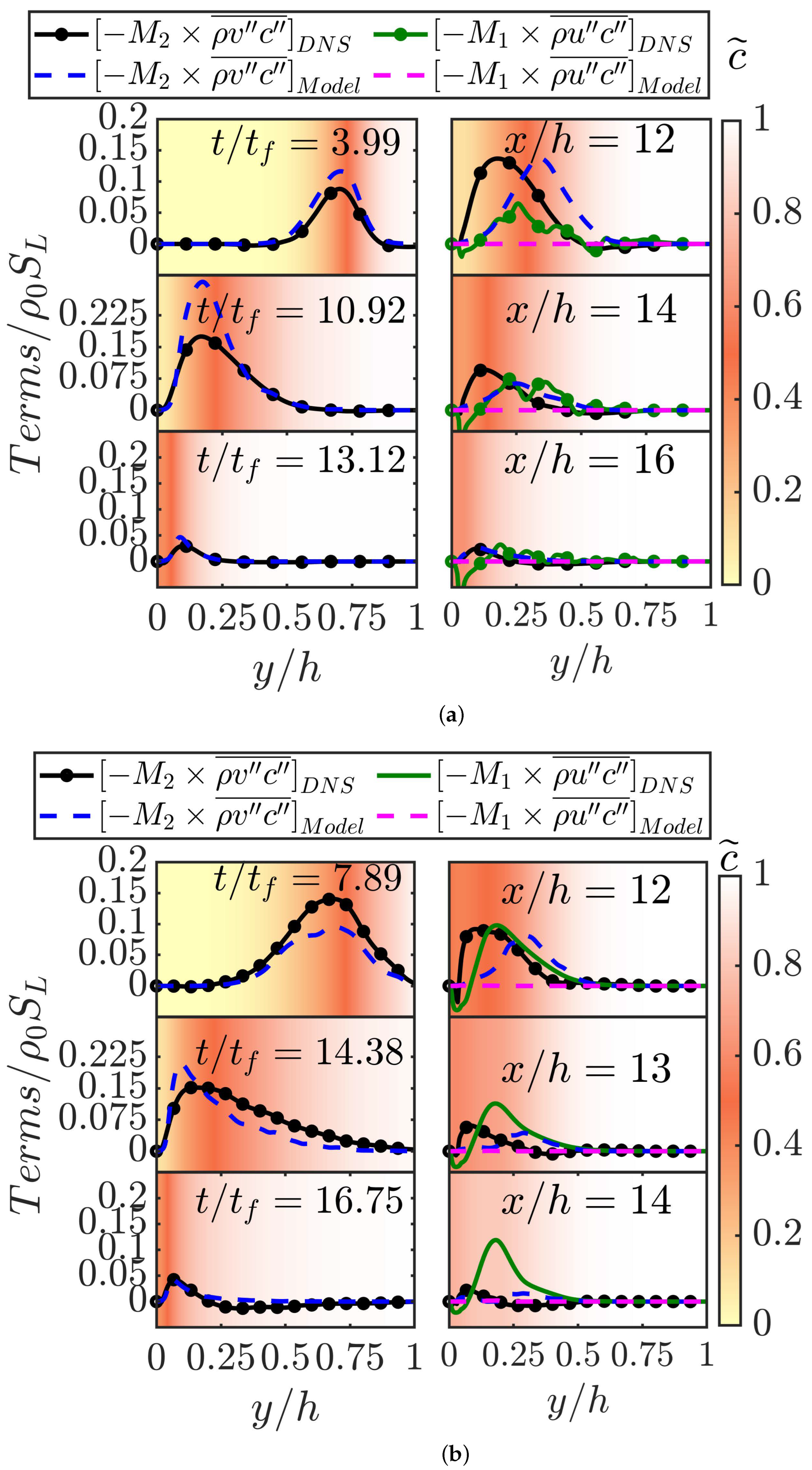
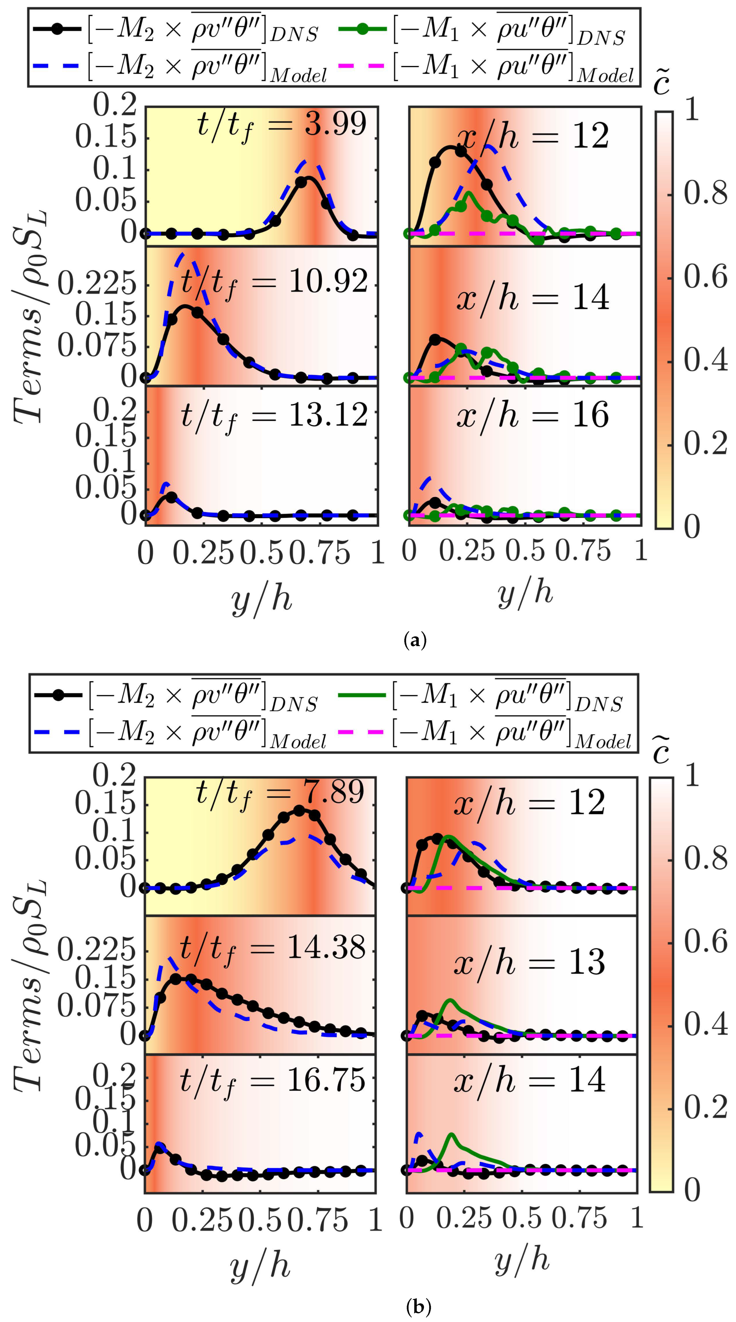
The unclosed turbulent transport term in Equation (1) involves the derivatives of the turbulent scalar flux components $\overline{\rho u_i^{″}{c}^{″}}$ and $\overline{\rho u_i^{″}{\theta }^{″}}$, and this is also valid for $\tilde{\theta }$ transport equation. Therefore, the model predictions of $\partial \overline{\rho u^{″}{c}^{″}}/\partial x$, $\partial \overline{\rho v^{″}{c}^{″}}/\partial y$, $\partial \overline{\rho u^{″}{\theta }^{″}}/\partial x$, and $\partial \overline{\rho v^{″}{\theta }^{″}}/\partial y$ were compared with the respective values derived from DNS data. The variations of $\partial \overline{\rho u^{″}{c}^{″}}/\partial x\times {\delta }_{th}/{\rho }_0{S}_L$, $\partial \overline{\rho v^{″}{c}^{″}}/\partial y\times {\delta }_{th}/{\rho }_0{S}_L$, and $\partial \overline{\rho u^{″}{\theta }^{″}}/\partial x\times {\delta }_{th}/{\rho }_0{S}_L$, $\partial \overline{\rho v^{″}{\theta }^{″}}/\partial y\times {\delta }_{th}/{\rho }_0{S}_L$ with $y/h$ along with the predictions of gradient of Equations (11) and (12) are shown in Figure 7 and Figure 8 for the HOQ and OWQ configurations, respectively. Here, it is worthwhile to note that only the wall normal component of the gradient of the scalar flux had a significant value even in the case of OWQ, as is expected for turbulent boundary layer flows. However, in the case of the HOQ configuration, the derivative of the streamwise component of the scalar flux was already zero for both the DNS and model predictions. The models given by Equations (11) and (12) provided reasonably accurate predictions of the behaviours of $\partial \overline{\rho v^{″}{c}^{″}}/\partial y$ and $\partial \overline{\rho v^{″}{\theta }^{″}}/\partial y$ at all stages of FWI in the V-flame OWQ case. The values of $\partial \overline{\rho u^{″}{c}^{″}}/\partial x$ and $\partial \overline{\rho u^{″}{\theta }^{″}}/\partial x$ obtained from DNS and model expressions in the OWQ case remained small, so the modelling inaccuracies in the prediction of $\overline{\rho u^{″}{c}^{″}}$ and $\overline{\rho v^{″}{\theta }^{″}}$ by models given by Equations (11) and (12) will not play a major role in RANS simulations.

In this work, a priori DNS assessment of algebraic closures of turbulent scalar flux for FWI within turbulent boundary layers has been considered. The suggested model expression has been found to demonstrate promising capabilities in capturing both the qualitative and quantitative behaviours of the turbulent scalar flux associated with the reaction progress variable and temperature for both configurations studied in the present work. This is especially important, because the standard gradient hypothesis model predicts the wrong sign of the scalar flux in the cases considered here. The quantitative deviations of the model predictions from the DNS data are not presented here because of their limited value and because this measure can vary from one case to another and at different locations/time instants for a given case. Furthermore, it could be misleading, because large errors in modelling $\overline{\rho u^{″}{c}^{″}}$ and $\overline{\rho v^{″}{\theta }^{″}}$ are of limited relevance in the channel flow configuration, as shown in Figure 7 and Figure 8.

5. Conclusions

The statistical behaviour and modelling of the turbulent fluxes of the reaction progress variable and non-dimensional temperature in the context of RANS during FWI in turbulent boundary layers have been analysed using three-dimensional DNS data. Two different DNS databases considered for this analysis were (i) statistically stationary OWQ of a V-shaped flame within a channel flow and (ii) unsteady HOQ of statistically planar flame propagating across a turbulent boundary layer. The main findings of the current analysis are the following:

• It has been found that the relative orientation of the flame with respect to the wall can affect the statistical behaviours of the scalar fluxes of the reaction progress variable and temperature during FWI.
• The standard gradient hypothesis has been shown to be inadequate for the closure of the turbulent fluxes of the reaction progress variable and temperature in both configurations.
• An existing algebraic scalar flux closure has been modified for FWI in this analysis, which is capable of predicting both gradient and counter-gradient types of transport depending on the underlying turbulent flow condition. This new model also includes the effects of the relative orientation of the flame with respect to the wall. The predictions of the newly proposed algebraic scalar flux closure have been demonstrated to capture both the qualitative and quantitative behaviours of the turbulent scalar fluxes of the reaction progress variable and temperature in the wall normal direction for both configurations.

It is worth noting that there is a lack of suitable experimental data for turbulent scalar flux during FWI in turbulent boundary layers. Therefore, directly comparing the current model predictions with experimental measurements is challenging. As such, experimental validation is beyond the scope of the current work. Nevertheless, this aspect remains an important avenue for future research endeavours. Once relevant experimental data become available, it should be utilised to validate and refine the model predictions. Therefore, experimental validation is left for future studies, where it can be pursued in greater depth and detail. Although the qualitative nature of the findings of this analysis is unlikely to be affected by the chemical mechanism, future analyses based on a broader range of operational parameters, including varied fuel types, equivalence ratios, and higher values of $R{e}_{\tau }$, will be needed for confirming the closures suggested in this analysis. Additionally, incorporating detailed chemistry and exploring higher Reynolds numbers will enhance the robustness and applicability of the proposed model. Furthermore, the newly proposed model expressions need to be implemented in RANS simulations for a posteriori assessment.