

Estimating the Deterministic and Stochastic Levelized Cost of the Energy of Fence-Type Agrivoltaics


1
Ocean Law and Policy Institute, Korea Institute of Ocean Science and Technology (KIOST), 385, Haeyang-ro, Yeongdo-gu, Busan 49111, Republic of Korea
2
School of Business, Pusan National University, 2, Busan Daehak-ro 63beon-gil, Geumjeong-gu, Busan 46241, Republic of Korea
*
Author to whom correspondence should be addressed.
Energies 2024, 17(8), 1932; https://doi.org/10.3390/en17081932
Submission received: 20 March 2024
/
Revised: 12 April 2024
/
Accepted: 14 April 2024
/
Published: 18 April 2024
(This article belongs to the Special Issue Feature Papers in Energy Economics and Policy)
Abstract
:Agrivoltaics can be used to supply energy and produce agricultural products in order to meet the growing demand for energy and food. The amount of power generation is affected by the solar panel direction, spacing, tilt, and panel technology; however, there is insufficient empirical data-based research on the operation of agrivoltaics. This study estimates the levelized cost of energy (LCOE) for a fence-based agrivoltaics system using bifacial modules. This study installed and operated photovoltaic (PV) systems on a rice paddy and saltern in South Korea to estimate the input variables that could affect their economic efficiency and LCOE. For the research methods, this study used Monte Carlo simulation (a stochastic analysis method that reflects the uncertainty of the input variables), a deterministic LCOE analysis, and a sensitivity analysis of the input variables. In terms of space utilization, the LCOE of the paddy system (139.07~141.19 KRW/kWh) was found to be relatively lower than that of the saltern system (145.43~146.18 KRW/kWh), implying that the PV system on the paddy was economically favorable. In terms of installation direction, it was more economical to operate the southwest-facing panels (139.07~145.43 KRW/kWh) than the southeast-facing panels (141.19~146.18 KRW/kWh). This study provides foundational policy data for the adoption of fence-based agrivoltaics and contributes to the widespread and active use of agrivoltaics.
1. Introduction
Energy demand is increasing rapidly worldwide due to industrialization and population growth; however, dependence on fossil fuels for energy generation remains high. Climate change caused by greenhouse gas emissions has reached an all-time high in weather observations over the past eight years. In 2022, global glacial thickness decreased by 1.3 m, thus increasing the rate of rising sea levels [1].
The number of photovoltaic (PV) system installations continues to grow as most countries, including developed countries, are increasing their share of power generation from renewable sources to reduce greenhouse gases [2]. Europe, as part of the Net-Zero Industry Act [3] and the Green Deal Industrial Plan for the Net-Zero Age [4], has set a target to increase the annual demand for net-zero technologies by at least 40% by 2030 via improving the manufacturing capacity for major net-zero technologies and expanding the regional production in the European Union (EU) [4]. At the 28th United Nations Climate Change Conference (COP28), held in December 2023, more than 130 countries agreed to triple their installed renewable energy capacity to at least 11,000 GW by 2030 [5]. Solar power generation is expected to surpass nuclear power generation by 2026, and renewable energy sources are expected to account for more than 42% of the global electricity generation by 2028. Solar power generation is expected to be economically advantageous because it is less expensive than conventional coal and natural gas [6,7].
The levelized cost of energy (LCOE) is a quantification of the cost of establishing and operating power generation facilities over their life cycle by energy source, which can be directly compared with other energy sources; it provides important basic data for decision making [8]. The expansion of solar power generation necessitates research on space utilization and capacity factors. Against this backdrop, this study estimates the LCOE in rural areas where PV systems, that is, agrivoltaics, have been installed.
In Europe, agrivoltaics and bifacial solar panels have recently emerged as a means through which to improve space utilization density in policies related to energy transition, agriculture, the environment, and research innovation [9]. Bifacial PV is more efficient and economical than monofacial PV, but it is affected by the operation type and its surrounding conditions [10,11,12,13,14,15,16,17]. Agrivoltaics can increase the economic value of rural areas, such as farming and fishing villages, and contribute to the decentralization and independence of electricity supply in rural areas [18]. Agrivoltaics have emerged as a promising solution to meet the increasing demand for energy and food due to population growth. A recent study on agrivoltaics reported that solar panel orientation, height, spacing, tilt, and panel technology affect agricultural production and energy generation [19].
An analysis of the research trends related to agrivoltaics shows that, according to the Scopus DB, 121 papers have been published on this topic, the majority of which were published in the last three years. Most of the research has been conducted in the United States and China, with a focus on short-term forecasting [20]. Mamun et al. analyzed operational issues and social impacts based on 83 studies on agrivoltaics in nine countries [21]. Nakata and Ogata estimated the potential of agrivoltaics and analyzed its direct and ripple effects [22]. However, the successful implementation of agrivoltaics requires social consensus, an institutional framework, and a mutual trust among the agricultural and fishery sectors and the government [23].
Amid the emergence of agrivoltaics in recent years, this study aims to provide foundational data for governments and civil society, including farmers and fishermen, by providing an objective LCOE based on practical operational results in rural areas. For the research methodology, this study used the Monte Carlo simulation method, a stochastic analysis method that considers the uncertainty of input variables; a deterministic methodology to conduct the LCOE estimation; and a sensitivity analysis by land use and installation type.
The marginal contributions of this study are as follows. First, an LCOE estimation investigation of agrivoltaics is carried out with a bifacial fence-based structure, which uses bifacial modules. Second, by distinguishing PV systems based on land use and installation orientation, this study analyzes cases under different conditions in rural areas. Third, this study reflects on the uncertainty related to the prerequisites by performing a stochastic analysis based on the data of empirical operations. Fourth, as most previous studies related to agrivoltaics have focused on crop fields and paddies, this study thus investigates the feasibility of using space for power generation in coastal areas by testing a PV system installed on a saltern. This study also aims to provide basic policy data for the adoption of agrivoltaics and contributes to the spread and active use of agrivoltaics.
2. Demonstration Agrivoltaics System
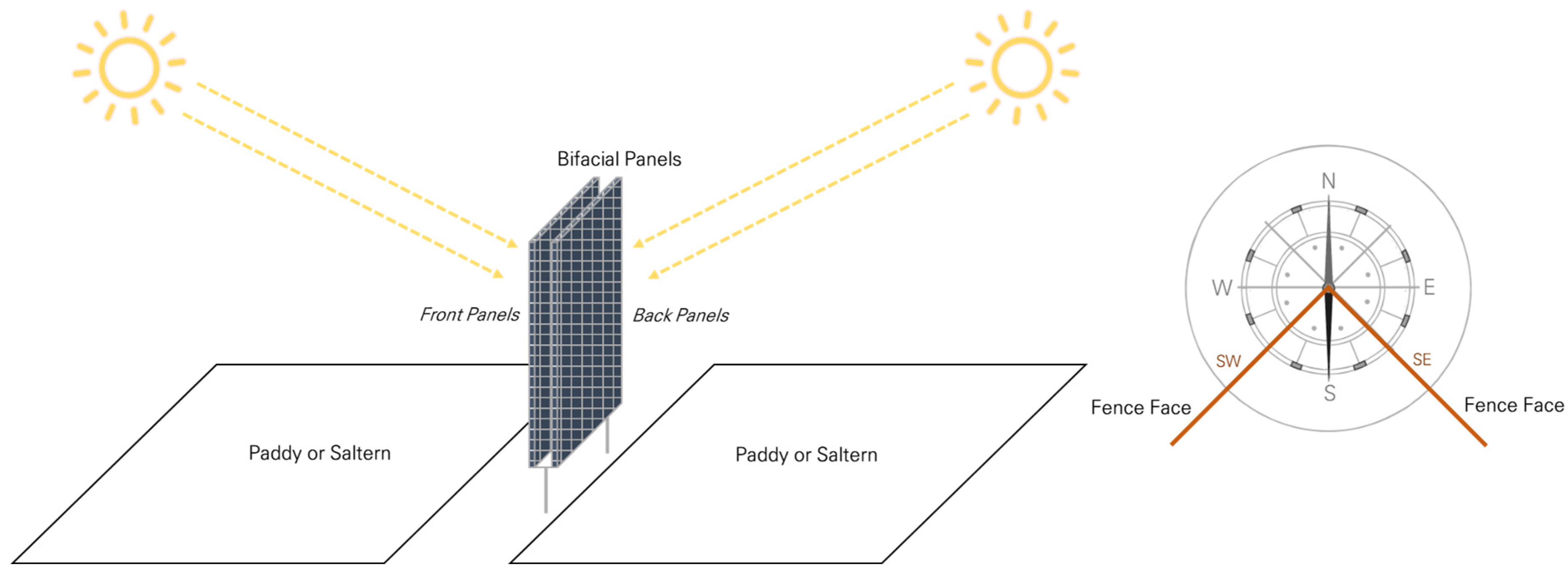
In this study, agrivoltaics systems were installed and operated upon in two locations: the western inland area of the Korean Peninsula and the coast of the Yellow Sea. Solar PV panels were installed using the space around an inland rice paddy and the space around a saltern on the coast. The solar PV structure of the demonstration plant was bifacial, as shown in Figure 1. Panels were installed on the front and back of the structure as a bifacial structure to increase the capacity factor. Solar radiation was absorbed according to the height of the sun, such that a PV system could be actively utilized [10,11,12,13,14,15,16]. The power generated by a bifacial PV system is significantly affected by the panel orientation [15,24,25,26]. In this study, bifacial PV systems were installed in paddy and saltern areas, and their practicality was improved by changing the panel orientation.
The studied paddy field is located inland, as shown in Figure 2, and it is surrounded by a large number of paddy fields. Diagonal-type and fence-type layouts were installed. Bifacial solar panels were operated in southeast–northwest and southwest–northeast directions.
As shown in Table 1, the agrivoltaics installed in the paddy had an installed capacity of 51.0 kW and consisted of 120 modules. The structure had two diagonal lines consisting of 42 fence units and 2 diagonal-type lines consisting of 18 fence units; the string configuration was 14 in series and 12 in series. The fence-based system was fully installed on 10 March 2022 and has been in operation since then.
The studied saltern system is located on the coast of the Yellow Sea, as shown in Figure 3, and it is surrounded by a large number of salterns. The installed layout included diagonal and straight types with bifacial solar panels facing the southeast–northwest and southwest–northeast directions.
As shown in Table 2, the agrivoltaics installed on the saltern had an installed capacity of 48.45 kW and consisted of 114 modules. The structure had a diagonal line consisting of 42 fence units, a mixed-type line (diagonal and straight) consisting of 36 fence units, and a straight line consisting of 18 fence units. It is a fence-based system, and it is similar to the agrivoltaics installed on the paddy. In addition, one line was added to the center part. The system was fully installed on 28 January 2022 and has been in operation ever since. Checks for the soil contamination caused by the operation of fence-based agrivoltaics showed that the concentrations of cations, such as Cd, Cu, As, Hg, Pb, Cr, Zn, and Ni, were below the standard values, thus implying that there was no need for environmental concern.
3. Literature Review
This study is about LCOE estimations for PV systems. This study estimated the actual power generation costs by assuming the life expectancy of PV systems. Previous studies on LCOE estimation can be divided into two main categories: research on the LCOE estimation for PV systems and research on the LCOE estimation for agrivoltaics.
First, this study reviewed the previous studies on the LCOE estimations for PV systems. In the United States, Mundada et al. estimated the LCOE for the following three renewable energy sources in the United States: PV, batteries, and CHP [27]; NREL estimated the LCOE considering the residential use, commercial use, performance degradation rates, and life cycle [28]; and Richelstein and Yorston estimated the LCOE of PV systems by size and panel type [29]. In Canada, Branker et al. estimated the LCOE of a PV system based on scenarios that adjusted the performance degradation rates and discount rates. Aquila et al. estimated the LCOE based on the conditional value at risk for microgeneration PV in 20 cities in Brazil, and they then compared it with the deterministic LCOE [30,31]. Ouyang and Lin estimated the LCOE for each energy type by categorizing the discount rates of 5%, 8%, and 10% based on the renewable energy generation data of 17 PV, wind, and biomass systems in China. In Thailand, Limmanee et al. estimated the LCOE by focusing on the performance degradation of PV modules [32,33]. In South Korea, Lee and Ahn estimated the LCOE by performing stochastic modeling using the capacity, capital expenditure, operations and maintenance (O&M) costs, discount rates, interest rates, and the economic life of a PV system as variables [34]. Lai and McCulloch estimated the LCOE of a hybrid system in Kenya that combined PV and electrical energy storage to determine its economic feasibility [35]. In Germany, Chudinzow et al. analyzed the interactions among installation parameters, such as energy yields in the north, south, east, and west directions; the LCOE; fixed tilt; module elevation; angle; and the soil reflectance for the cost-optimal design of bifacial PV [36]. In Italy, Bianco et al. estimated the LCOE of a PV system based on a renewable energy technology policy and showed that certain factors, such as incentives and market prices, have a significant impact [37]. In Spain, Rodríguez-Osorio et al. performed the LCOE and sensitivity analyses using variables such as financing interest rate, capital cost, operating cost, plant performance, and the life expectancy of a PV system [38]. In Finland, Väisänen et al. estimated the changes in the LCOE based on the size of a PV system’s inverter [39].
A transnational study suggested LCOE-based metrics to investigate appropriate subsidies or incentives for building-integrated photovoltaics (BIPV) in European capitals, including Norway and Switzerland [40]. Reichenberg et al. estimated and compared the LCOE of PV and wind power generation in Europe by considering weather conditions and costs in Europe [41]. Bartiainen et al. estimated the LCOE of PVs in Helsinki, London, Munich, Toulouse, Rome, and Malaga [42], while Ondraczek et al. estimated the LCOE for 143 countries by considering solar radiation and capital costs [43].
In summarizing the findings of previous studies on the LCOE estimation for PV systems, this study found that the discount rate used for estimation varied from a minimum of 2% to a maximum of 11.4%, where the lifetime was assumed to be 15–32 years. As a research method, Gholami and Røstvik (2021) and Her-Nández-Moro and Martínez-Duart (2013) presented the results of an NPV analysis along with the LCOE, and Agostini et al. (2021) performed NPV and IRR analyses [40,44]. Branker et al. (2011), Chudinzow et al. (2020), Hernández-Moro and Mar-tínez-Duart (2013), Lee and Ahn (2020), Mundada et al. (2016), Ondraczek (2014), Reichel-stein and Yorston (2013), Reichenberg et al. (2018), Rodríguez-Ossorio et al. (2021), and Var-tiainen et al. (2020) performed sensitivity analyses on the LCOE to evaluate the influence of key variables [27,31,34,36,38,41,42,44,45].
Second, we reviewed the studies on LCOE estimation for agrivoltaics that investigated the optimal PV systems and agricultural crop varieties by simultaneously operating crop production and solar power generation systems. In Europe, Feuerbach et al. estimated the LCOE by comparing vegetable and cereal farms in Germany, and their sensitivity analysis showed that insolation and investment costs were the main factors; moreover, they also estimated the LCOE of agrivoltaics for crops, milk production, and granivores [46]. Schindele et al. compared and evaluated the costs of agrivoltaics and ground-mounted PV, and they found that it was economically favorable to grow crops and operate PV at the same time, but not in the case of wheat cultivation [47]. In Germany, Thomas et al. estimated energy and agricultural production by setting up scenarios based on the angle of solar panels. They also estimated the impact of a large-scale PV project by considering social, socioeconomic, and environmental impacts, and climate change [48]. Trómsdorf et al. estimated the LCOE of a PV system in an apple orchard [49]. In Italy, Agostini et al. conducted an environmental and economic assessment of agrivoltaics by including their impact on ecosystems, air quality, and climate change, and they also evaluated their contribution to sustainable development goals [50]. France and Cupo conducted a cost–benefit analysis and an LCOE estimation for utility-scale agrivoltaics for different regions and crop types such as durum wheat, soft wheat, corn, sunflower, soybean, and potato [51]. In the United States, Cupari et al. estimated the LCOE by performing stochastic modeling simulations for agrivoltaics located on alfalfa and soybean farms in Oregon, as well as on soybean and strawberry farms in North Carolina [52]. Dinesh and Pearce argued that the economic value of a farm increases by more than 30% when agrivoltaics are used instead of traditional agricultural practices [53]. In Niger, Bhandari et al. estimated and compared the LCOE of energy production facilities using diesel engines and PV systems on salad, cabbage, tomato, and mint farms [54]. Poonia et al. estimated the LCOE of PV systems according to one-, two-, and three-row array structures in India [55]. Thomas et al. set up scenarios based on the angles of solar panel to consider energy production and agricultural production in Asia, and they also evaluated the impact of large-scale PV projects by considering their social, socioeconomic, and environmental impact, as well as climate change [48].
Ahmed et al. conducted economic and environmental assessments of agrivoltaics systems in Vietnam, Bangladesh, India, China, Egypt, and Brazil; they estimated the LCOE of PV systems on farms in each country and found that PV systems are affected by panel tilt. In addition, they established that bifacial panels can increase profits by 18 to 35% over monofacial panels [56]. Junedi et al. found that the LCOE of agrivoltaics was significantly affected by factors such as life cycle, module efficiency, structural support, occupied space, installation type, PV location, and solar radiation, and they also estimated the LCOE based on the location of the agrivoltaics, rooftops, and buildings [57]. Hayibo and Pearce estimated the LCOE by considering panel tilt and seasonal factors [58], and Willockx et al. suggested using the LCOE and optimal ground coverage ratio for the entire EU using geospatial data [59].
Our review of previous LCOE studies on agrivoltaics shows that the research was conducted mainly in advanced countries, such as the United States, Germany, and Italy, and the LCOE was estimated based on solar power generation and crop production according to crop type. This study considers the analysis methods and variables used in the aforementioned studies (see Table 3 for a summary). This study differs from previous studies in that it analyzes the amount of solar power generated according to land use and installation type. Furthermore, the LCOE of agrivoltaics reflects the uncertainty of the input variables when using a stochastic simulation methodology, and this is because the economic conditions, capacity, installation cost, and O&M costs differ by country and region. This is an LCOE estimation study on an agrivoltaics demonstration project in South Korea, which also needs to be conducted in other countries for the purposes of comparative analysis.
4. Materials and Methods
4.1. Levelized Cost of Energy
In this study, the LCOE of PV refers to the average real cost of generating electricity per kilowatt (kW) of unit power, and it is calculated by dividing the total cost of the power generation facility by the total power generation based on the present value. The LCOE takes into account costs incurred throughout the process, such as initial capital expenditures (CAPEX), as well as operation, maintenance, and decommissioning costs in the facility’s lifetime. The LCOE is affected by CAPEX, O&M, lifetime, capacity factor, degradation rate, inflation rate, interest rate, tax rate, debt fraction, and debt term and the calculation method can be defined as shown in Equation (1) [25,37,44,48,49,50,51,59]. This study excludes the benefits of government support such as renewable energy certificates (RECs) and incentives.
where CAPEX is divided into direct and indirect costs. The major direct cost items include the modules, inverters, spiral structure material production, structure and module installation work, electrical materials, and line construction. Indirect cost items include development activities, design, supervision, structural safety diagnosis, pre-use inspection, regulatory affairs, REC bidding, licensing, indirect labor, general management, and other expenses. refers to the maintenance cost for year n, refers to the PV system’s operating period. refers to the financing cost for n, and is the discount rate, which, in this study, refers to the weighted average costs of capital (WACC). For the LCOE of the PV system, this study applies the discount rate r to the costs incurred during the PV system’s lifetime—in other words, the same amount of money is recovered every year.
4.2. Stochastic Approach
The research methodology used in this study, Monte Carlo simulation, is a commonly used stochastic simulation method [63]. Input variables are selected to estimate the LCOE of the PV system by type. For the input variables, variables with high uncertainty are set as random variables, and the random variables are estimated by assuming an appropriate random distribution. The range and probability of the expected value are calculated by extracting the random number for each random variable. The expected value, which is an output variable in this study, is the LCOE for each type. Specifically, the random variable of the Monte Carlo simulation has a probability density function . By assuming an arbitrary function , and then integrating it, the expected value of can be calculated, as shown in Equation (2):
To estimate the expected value of , n samples () are extracted from the distribution of random variables , and the mean of is calculated using Equation (3). The distributions of random variables include normal, triangular, logistic, Bernoulli, beta, binary, and exponential distributions, as well as the probability weights, are assigned differently according to the distribution [64]. In this study, an appropriate distribution is assumed for each random variable in the LCOE estimation to perform the analysis [34].
In Monte Carlo simulation, the estimate of the expected value is the Monte Carlo estimator of , which is based on the law of large numbers. If expressed based on the weak law of large numbers, as shown in Equation (4), the mean of for the sample converges to , which is when the number of samples becomes infinite. In this study, the range and probability are derived by repeating the random number extraction 10,000 times [34].
When sampling is repeated infinitely, the probability that the absolute value of the error is zero becomes 1. In addition, satisfies Equation (5) and becomes an unbiased estimator of .
4.3. Sensitivity Analysis
A sensitivity analysis is a method used to analyze the change (contribution) in an expected value, which is achieved by changing only one variable among the random variables defined with the probability distribution in the simulation and keeping the remaining random variables fixed. In other words, by identifying the variables that affect the simulation results, the relative ranking of the direction and magnitude of the effects of the random variables on the LCOE can be compared through a sensitivity analysis of the LCOE contribution of the PV. This study used the Crystal Ball program for its sensitivity analysis. The process of calculating the variance contribution is shown in Equation (6) [65].
First, the samples and results of the input variables derived by the Monte Carlo simulation were ranked to derive the rank correlation coefficient between the input variable samples and results [65,66,67]. Next, the variance contribution of the input variable was introduced to represent the proportion of , which is the square of the rank correlation coefficient, to the sum of the square of each of the rank correlation coefficients, as shown in Equation (6):
where the rank correlation coefficient in the numerator uses conventional negative (−) and positive (+) signs. If the rank correlation coefficient is positive (+), the result will increase as the input variable increases. If the sign is negative (−), the result will decrease as the value of the input variable increases. Therefore, the degree and direction of the impact of the input variables on the LCOE estimation can be determined through a sensitivity analysis.
5. Results
5.1. Data
This study categorized agrivoltaics based on land use and solar panel orientation to estimate the LCOE. This study classified the following four orientations: southeast and southwest on the paddy, and southeast and southwest on the saltern. In the case of the paddy, a 15.3 kW power plant was operated for the southeast orientation, while 17.85 kW and 15.30 kW power plants were operated for the southwest orientation. In the case of the saltern, six 2.55 kW power plants were operated for the southeast orientation, and 17.85 kW and 15.30 kW power plants were operated for the southwest orientation.
As for the input data, as shown in Table 4, there were different factors for each type, as well as commonly applied factors. The main factors for estimating the LCOE included discount rate, tax, performance degradation rate, interest rate, inflation rate, and lifetime, which were applied regardless of the type. This study assumed the degradation rate, inflation rate, and corporate tax, which have relatively low uncertainties, were deterministic variables. For the capacity factor, CAPEX, O&M costs, discount rate, and interest rate, which are items with high uncertainty, this study applied a probabilistic method by using the distribution of previous studies [34].
5.1.1. Deterministic Variables
In this study, the deterministic variables included capacity factor, CAPEX, O&M, decommissioning costs, and interest rates. The capacity factor for the demonstration of the PV system was based on the annual power generation (including downtime) from 1 June to 31 May 2023. CAPEX was understood as the total capital expenditure on the PV equipment installed in each power plant, and O&M was used to refer to the total annual O&M costs. For interest expenses, this study assumed a debt term of 10 years and an annual interest rate of 3%, which is in line with the typical form of project financing at the time of construction. For corporate tax, this study assumed that 11.0% of annual power generation revenue, after deducting O&M, interest expenses, and depreciation, would be paid for 20 years. In other words, a certain percentage of the income generated from the operation of the power generation business was paid as tax. Although there were also cases where the tax was reduced or exempted depending on the power generation scale and region, assuming a common situation, this study used the typical corporate tax rate of 11.0% in South Korea for the analysis. The inflation rate was fixed at 1.72%. The degradation rate refers to the performance degradation of a PV system over time, which has a significant impact on power generation. The average performance degradation rate of a PV system is 0.2% to 0.8%; in this study, it was assumed to be 0.6% [27,31,34,35,36,40,61].
5.1.2. Stochastic Variables
This study performed the simulations by assuming a probability distribution for variables with high uncertainty. The variables assumed to have a probability distribution were the capacity factor, CAPEX, O&M costs, discount rate, and interest rate after considering previous studies and the results of the demonstration operation. The variables were greatly affected by the orientation of the solar panels and the surrounding environment, such as salt ponds and rice paddies.
The capacity factor is an important factor when analyzing the cost of power generation and can be affected by the location of the power plant, amount of solar radiation, the surrounding environment, and panel orientation. Lee and Ahn (2020) derived an optimal distribution using the capacity factor data of all the PV plants in South Korea and found that the capacity factor followed a logistic distribution with a scale of 0.22%. Similar to Lee and Ahn (2020), this study assumed a logistic distribution for the capacity factor, with the mean being the actual value obtained in this study, which had a scale of 0.22%.
In the case of CAPEX, the normal distribution is known to be the most appropriate. This study assumed a mean value of 1,350,973.49 KRW/kW with a standard deviation of 135,097, which is 10% of the mean. For O&M, this study assumed a normal distribution with a mean of 29,010 KRW/kW and standard deviation of 2901, which is 10% of the mean [34]. The discount rate was calculated based on a concept that converts future cash value into a present value, and it is a very important factor to consider in LCOE estimation. Lee and An (2020) determined that the discount rate showed a high goodness of fit in the triangular distribution. In this study, this study assumed a likelihood of 4.5%, a minimum of 4.5%, and a maximum of 7.5%, which are in line with Lee and An (2020). The interest rate is financing costs incurred during actual operation. Because the minimum and maximum values were clear, this study assumed a triangular distribution. In addition, because the Bank of Korea’s minimum and maximum base rates for the past five years were 0.5% and 3.5%, respectively, this study assumed a most likely rate of 3.0%, a minimum of 0.5%, and a maximum of 3.25% [34,68].
5.2. Results of the Levelized Cost of Energy Analysis
5.2.1. Results of the Deterministic Analysis
Table 5 presents the results of estimating the LCOE of agrivoltaics using a deterministic method. When agrivoltaics were operated with the installed solar panels facing southwest, the LCOE was 134.15 KRW/kWh for the paddy and 140.48 KRW/kWh for the saltern. In the case of the southeast orientation, the LCOE was 136.27 KRW/kWh for the paddy and 141.32 KRW/kWh for the saltern. Overall, the LCOE of the agrivoltaics installed in the southwest orientation was lower than that of the southeast orientation, thus making it more economically viable.
The agrivoltaics installed in the paddy with a southwest orientation had the lowest LCOE at 134.15 KRW/kWh, making it the most economically favorable. The agrivoltaics installed on the saltern with a southeast orientation had the highest LCOE at 141.32 KRW/kWh; however, this was due to incoming voltage inconsistency due to road construction activities outside the saltern, which caused frequent shutdowns of the inverter part. Therefore, the LCOE of the saltern could be lower than that of the paddy if there are no technical problems. This is because saltern are typically operated in areas with high solar radiation.
This study also estimated the LCOE for each input variable by decomposing the LCOE based on the factors. Owing to the low power generation of the saltern, the LCOE of the saltern CAPEX (90.99 KRW/kWh to 91.62 KRW/kWh) was higher than that of the paddy CAPEX (86.25 KRW/kWh to 87.84 KRW/kWh). It accounted for about 65% of the total LCOE. The LCOE from O&M was approximately 30 KRW/kWh and accounted for 22% of the total LCOE. Decommissioning costs accounted for 0.1% (0.18 KRW/kWh to 0.19 KRW/kWh); financing costs accounted for 8% (10.44 KRW/kWh to 11.63 KRW/kWh); and tax accounted for 6% (7.59 KRW/kWh to 8.26 KRW/kWh).
5.2.2. Deterministic Analysis Results
Using the Monte Carlo simulation method, this study assumed the probability distribution for the variables with uncertainty and volatility among the input data of the PV system. Within the set distribution, an arbitrary random number was repeated 10,000 times, and the LCOE range of the PV system was estimated at a 95% confidence interval. Table 6 and Figure 4 present the stochastic analysis results of the LCOE of the paddy and saltern in the southwest and southeast orientations, respectively. The baseline values refer to the results of the deterministic analysis.
The LCOE of the paddy in the southeast orientation had a mean value of 141.19 KRW/kWh, a standard deviation of 11.96 KRW/kWh, a minimum value (based on 2.5%) of 118.58 KRW/kWh, and a maximum value (based on 97.5%) of 165.27 KRW/kWh. The southwest orientation had a mean value of 139.07 KRW/kWh, a standard deviation of 11.70 KRW/kWh, a minimum value of 116.77 KRW/kWh, and a maximum value of 162.96 KRW/kWh. In the case of the saltern, the LCOE for the southeast orientation had a mean value of 140.48 KRW/kWh, a standard deviation of 12.42 KRW/kWh, a minimum value of 122.95 KRW/kWh, and a maximum value of 172.08 KRW/kWh. In contrast, the LCOE for the southwest orientation had a mean value of 145.43 KRW/kWh, a standard deviation of 12.42 KRW/kWh, a minimum value of 122.35 KRW/kWh, and a maximum value of 171.46 KRW/kWh.
In the deterministic analysis, the saltern with the southeast orientation accounted for the highest estimated LCOE, which was followed by the saltern with a southwest orientation, the paddy with a southeast orientation, and the paddy with a southwest orientation. In the Monte Carlo simulation, the mean values were similar. In terms of the standard deviations, the saltern with a southeast orientation showed the highest value (12.47), and the paddy with a southwest orientation showed relatively low variation (11.70). The coefficient of variation was 0.09 for the saltern and 0.08 for the paddy, thereby showing an insignificant difference.
5.2.3. Results of the Sensitivity Analysis
According to the sensitivity analysis results of the LCOE of the PV systems, as shown in Table 7, the CAPEX had the highest impact, ranging from 65.9% to 66.6% for all types of PV systems. CAPEX is the most important economic factor when operating a PV system, and technical and institutional improvements are required to reduce costs [46]. The second most important factor was the discount rate, which was followed by the capacity factor and O&M. The interest rate had the least impact. The discount rate reflects the financial and social environmental factors, as well as accounts for a significant proportion of the population.
While most of the factors had a positive impact, the capacity factor had a negative impact. In other words, the higher the capacity factor, the lower the LCOE. In particular, the saltern with a southeastern orientation exhibited a value of 8.9%, thereby accounting for the largest impact. Therefore, as the improvement of the capacity factor has a positive effect on the reduction in LCOE, it must be accompanied by technical improvements or environmental conditions to reduce costs [11].
6. Discussion and Conclusions
This study aims to compare the LCOE of agrivoltaics with previous research findings in order to assess the relative magnitude of LCOE based on land use. Through this comparative analysis, the objective is to economically evaluate the advantageous land utilization patterns, including paddy, salt, and farm lands, by examining the estimated LCOE up to the present period. Therefore, by comparing the levels of LCOE, this study assessed the economic viability of salt fields and paddy fields, which are the subjects of this research. Table 8 shows the results of the empirical LCOE analysis for agrivoltaics compared with those of previous studies. The results vary depending on the crop type (winter wheat, corn, canola, barley, rye, potatoes, and apples), solar panel type, and incentives. In previous studies, the LCOE of agrivoltaics was affected by the country, location, economic conditions, capacity factor, CAPEX, O&M, etc. [69,70,71].
Hayibo and Pearce assumed a discount rate of 4.1% [58], whereas Poonia et al. assumed a discount rate of 12.0% [55]. For the degradation rate, the estimation conditions varied significantly, ranging from 0.25%, a value assumed by Feuerbacher et al. [62], to 3.10%, a value assumed by Trommsdorff et al. [49]. For the lifetime factor, the values ranged from a minimum of 25 years [48,50,54,59,62] to a maximum of 30 years [49,53]. In this study, the lifetime was set to 20 years because PV is institutionally guaranteed in South Korea; however, as the economic lifetime increases to at least 25 years, owing to the development of PV module technology, it is possible that the LCOE results of this study could be further reduced. Therefore, the results of this study can be interpreted as conservative.
For a realistic comparison between the LCOE estimates of the paddies and salterns, this study considered the real price in 2023 as the base year, as shown in Equation (7). When applying the real price, Year A refers to the publication year of each previous study, and the analysis is performed based on the exchange rate and consumer price index (CPI) of the pertinent year. The estimates of previous studies were analyzed considering the CPI of the country as of 2023 [72,73].
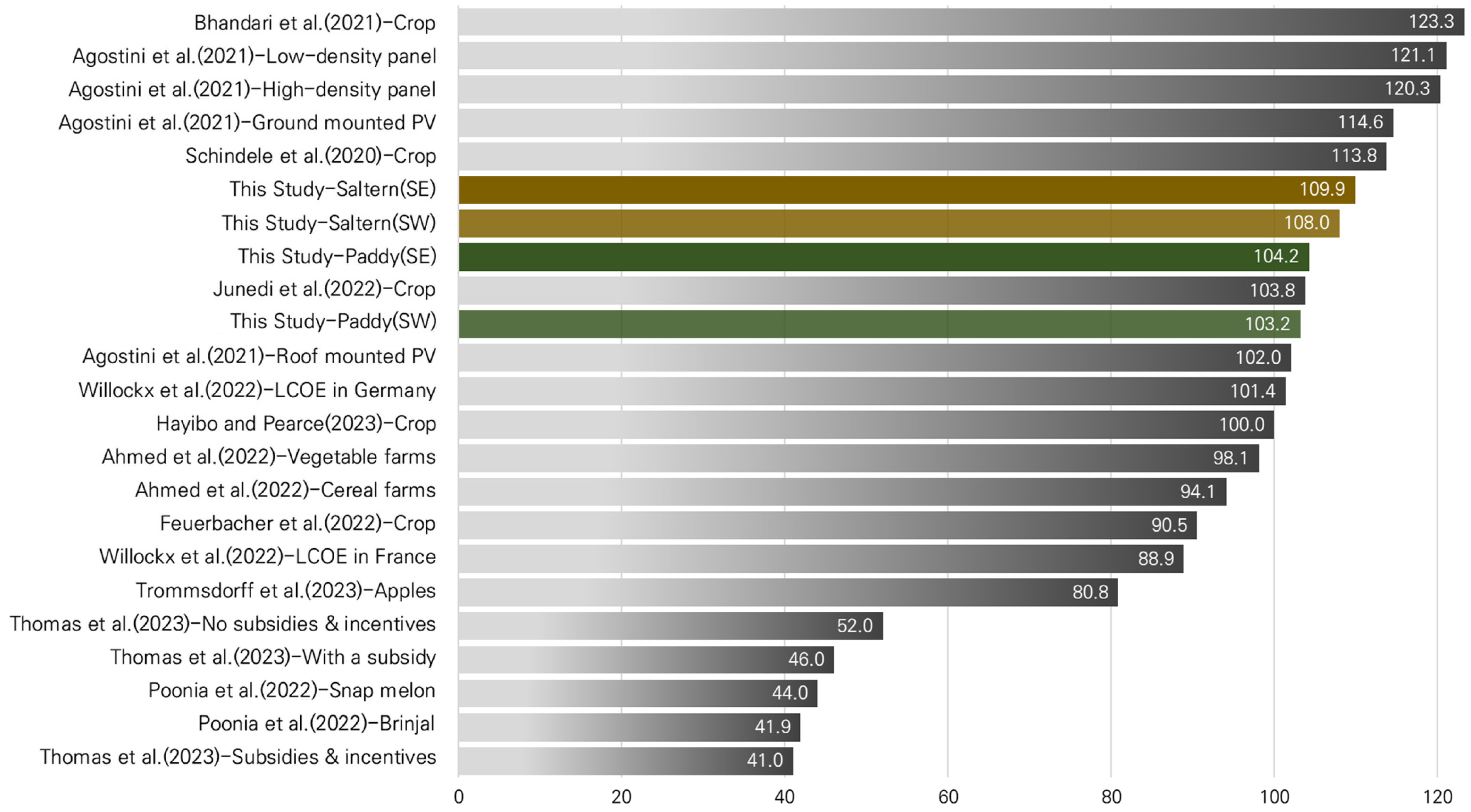
When the LCOE estimates of previous studies were combined, the mean was 100.9 USD/MWh. The LCOE estimates in this study ranged from a minimum of 103.2 USD/MWh to a maximum of 109.9 USD/MWh, which is slightly higher than the mean of previous studies in Figure 5. The LCOE estimated by Dinesh and Pearce for a lettuce farm in the United States was the highest (318.7 USD/MWh) [53], which is followed by the LCOE estimated by Bhandari et al. for PV systems in millet, sorghum, cowpea, and peanut farms (123.3 USD/MWh) [54]. India accounted for the lowest LCOE among the countries analyzed as the LCOE estimated by Poonia et al. was 41.9 USD/MWh for brinjal farms and 44.0 USD/MWh for snap melon farms [55]. The LCOE estimated by Thomas et al., which took subsidies and incentives into consideration, was 41.0 USD/MWh [48]. Different countries have different conditions that affect PV costs, and the LCOE is affected by land use and the type of agrivoltaics used.
While the worldwide dependence on fossil fuels for energy remains high, most countries, including developed countries, are expanding their support for renewable energy and increasing their share of power generation from renewable sources to reduce greenhouse gas emissions. As the number and size of PV installations continue to increase, agrivoltaics are emerging as a means of meeting the growing demand for energy and food. In terms of land use, agrivoltaics have the advantage of being able to generate energy and produce agricultural products at the same time. The power generation of agrivoltaics is affected by their orientation, spacing, tilt, and solar panel technology. However, there is a lack of research based on empirical data regarding the actual operation of agrivoltaics.
Previous studies have primarily evaluated the LCOE in farm settings (vegetables, cereals, etc.), whereas this study estimated the realistic LCOE of agrivoltaics by considering the distinctiveness of land use (paddy fields and salt fields), installation type (bifacial panel and fence-type), and operational methods (panel direction).
This study estimated the LCOE of PV systems with a fence-based structure using bifacial modules under various conditions in rural areas by classifying the land use and installation type (orientation) of the PV systems. Specifically, the bifacial PV systems were operated in rural areas, and the degree of influence of the variables that could affect the systems’ economic feasibility was identified based on the operation results. This study was conducted to ensure the economic feasibility of agrivoltaics and improve their operational efficiency.
This study used the Monte Carlo simulation method, a stochastic analysis method that is used to estimate the LCOE by land use and installation type, and it was conducted with a sensitivity analysis of the input variables. As for the input variables for the stochastic analysis, this study assumed appropriate probability distributions for the capacity factor, CAPEX, discount rate, and interest rate, as well as fixed the values of the degradation rate, inflation rate, and corporate tax, which have relatively low uncertainties.
First, the deterministic analysis of the LCOE that focused on land use showed that the LCOE of the paddy was in the range of 134.15 KRW/kWh to 136.27 KRW/kWh and the LCOE of the saltern was in the range of 140.48 KRW/kWh to 141.32 KRW/kWh, regardless of the installation orientation. However, because of a technical problem with the saltern PV system, it cannot be generalized that the LCOE of the saltern PV system was higher than that of the paddy PV system.
Meanwhile, when comparing the installation orientation, this study found that the maximum LCOE was 140.48 KRW/kWh when the PV system was operated with a southwest orientation and 141.32 KRW/kWh when it was operated with a southeast orientation. This suggests that a southwest orientation facilitates a relatively high economic efficiency. Therefore, considering the installation orientation, it is economically advantageous to operate bifacial module agrivoltaics with a southwest orientation and disadvantageous to operate with a southeast orientation.
Similar to the results of the deterministic analysis, the stochastic analysis shows that the LCOE is relatively low for paddy fields in terms of land use and southwest orientation in terms of installation orientation. This means that it is economically favorable to operate agrivoltaics with a southwest orientation in paddy fields.
Based on the LCOE, the southwest-oriented paddy was the most economically favorable (139.07 KRW/kWh), which was followed by the southeast-oriented paddy (141.19 KRW/kWh), the southwest-oriented saltern (145.43 KRW/kWh), and southeast-oriented saltern (146.18 KRW/kWh). By performing a simulation considering the probability distributions of the input variables, the mean LCOE estimate was found to be approximately 5 KRW/kWh higher than the deterministic LCOE estimate. This is because the LCOE estimate was determined based on changes in the random number according to the distribution of the variable.
The sensitivity analysis of the LCOE of agrivoltaics revealed that CAPEX had the highest impact, ranging from 68.6% to 69.8% in all of the types of PV systems; this was followed by the discount rate, capacity factor, O&M, and interest rate, which had the lowest impact. In contrast, while most factors had a positive impact, the capacity factor had a negative impact. When this study performed a comparison based on land use, this study found that the influence of O&M was 4.0–4.5% on the paddy and 4.8–5.1% on the saltern. This suggests that the O&M costs are relatively important variables in the operation of agrivoltaics. In summary, from an economic perspective, the technology development and support that reduce CAPEX are favorable for ensuring the economic viability of agrivoltaics, and efforts to improve the capacity factor are also required.
In conclusion, among the four types of bifacial modules (southwest and southeast orientations on the paddy, and southwest and southeast orientations on the saltern), the southwest orientation improved the operation’s capacity factor, thus suggesting that panel orientation is a very useful factor in reducing the LCOE. According to the findings of this study, the LCOE of agrivoltaics averages 100.9 USD/MWh, which appears relatively high for solar PV systems operating in salt fields and paddy regions. However, considering the long-term operation and the production of salt and rice, it appears to be economically advantageous. The results of this study will contribute to the provision of basic policy data for the adoption of bifacial, fence-type agrivoltaics, as well as to the spread and active use of PV systems.
A limitation of this study was that it was conducted in the early stages of the demonstration operation and mainly focused on the southwest and southeast orientations. In the future, it will be necessary to expand and operate other azimuths to diversify the types and operational agrivoltaics over the long term. Furthermore, it is necessary to conduct a comprehensive economic analysis that reflects the benefits of fence-type agrivoltaics and their impact on the crop or salt production losses that may occur in salterns and paddies.
Author Contributions
Conceptualization, C.-Y.L.; methodology, C.-Y.L.; software, K.-W.H.; validation, K.-W.H.; formal analysis, K.-W.H.; investigation, C.-Y.L.; resources, C.-Y.L.; data curation, C.-Y.L.; writing—original draft preparation, K.-W.H.; writing—review and editing, C.-Y.L.; visualization, K.-W.H.; supervision, C.-Y.L.; project administration, C.-Y.L.; funding acquisition, C.-Y.L. All authors have read and agreed to the published version of the manuscript.
Funding
This research was funded by Korea Energy Technology Evaluation and Planning (grant number 20213030010140).
Data Availability Statement
Data are unavailable due to privacy.
Conflicts of Interest
The authors declare no conflicts of interest.
References
- WMO. State of the Global Climate 2022. 2023. Available online: https://library.wmo.int/records/item/66214-state-of-the-global-climate-2022 (accessed on 1 February 2024).
- WMO-IRENA. 2022 Year in Review: Climate-Driven Global Renewable Energy Potential Resources and Energy Demand. 2023. Available online: https://storymaps.arcgis.com/stories/6e4e1e4985eb4a79b9037c258f6acb71 (accessed on 1 February 2024).
- European Commission. EU Net-Zero Industry Act: Making the EU the Home of Clean Tech Industries. 2023. Available online: https://single-market-economy.ec.europa.eu/publications/net-zero-industry-act_en (accessed on 1 February 2024).
- European Commission. Communication-A Green Deal Industrial Plan for the Net-Zero Age. 2023. Available online: https://commission.europa.eu/document/41514677-9598-4d89-a572-abe21cb037f4_en (accessed on 1 February 2024).
- COP28 World Climate Action Summit, Dubai, United Arab Emirates, 1–2 December 2023. Available online: https://www.consilium.europa.eu/en/meetings/international-summit/2023/12/01-02/ (accessed on 1 February 2024).
- IEA. Renewables 2023-Analysis and Forecast to 2028. 2024. Available online: https://www.iea.org/reports/renewables-2023 (accessed on 1 February 2024).
- IRENA. Renewable Power Generation Costs in 2022, International Renewable Energy Agency, Abu Dhabi. 2023. Available online: https://www.irena.org/Publications/2023/Aug/Renewable-Power-Generation-Costs-in-2022 (accessed on 1 February 2024).
- IEA. Projected Costs of Generating Electricity 2020. 2020. Available online: https://www.iea.org/reports/projected-costs-of-generating-electricity-2020 (accessed on 1 February 2024).
- Chatzipanagi, A.; Taylor, N.; Jaeger-Waldau, A. Overview of the Potential and Challenges for Agri-Photovoltaics in the European Union; Publications Office of the European Union: Luxembourg, 2023; JRC132879. [Google Scholar] [CrossRef]
- Guerrero-Lemus, R.V.T.K.A.K.L.S.R.; Vega, R.; Kim, T.; Kimm, A.; Shephard, L.E. Bifacial solar photovoltaics–A technology review. Renew. Sustain. Energy Rev. 2016, 60, 1533–1549. [Google Scholar] [CrossRef]
- Gu, W.; Ma, T.; Ahmed, S.; Zhang, Y.; Peng, J. A comprehensive review and outlook of bifacial photovoltaic (bPV) technology. Energy Convers. Manag. 2020, 223, 113283. [Google Scholar] [CrossRef]
- Lamers, M.W.P.E.; Özkalay, E.; Gali, R.S.R.; Janssen, G.J.M.; Weeber, A.W.; Romijn, I.G.; Van Aken, B.B. Temperature effects of bifacial modules: Hotter or cooler? Sol. Energy Mater. Sol. Cells 2018, 185, 192–197. [Google Scholar] [CrossRef]
- Patel, M.T.; Khan, M.R.; Sun, X.; Alam, M.A. A worldwide cost-based design and optimization of tilted bifacial solar farms. Appl. Energy 2019, 247, 467–479. [Google Scholar] [CrossRef]
- Rodríguez-Gallegos, C.D.; Bieri, M.; Gandhi, O.; Singh, J.P.; Reindl, T.; Panda, S.K. Monofacial vs bifacial Si-based PV modules: Which one is more cost-effective? Sol. Energy 2018, 176, 412–438. [Google Scholar] [CrossRef]
- Appelbaum, J.J.R.E. Bifacial photovoltaic panels field. Renew. Energy 2016, 85, 338–343. [Google Scholar] [CrossRef]
- Fertig, F.; Krauß, K.; Greulich, J.; Clement, F.; Biro, D.; Preu, R.; Rein, S. The BOSCO Solar Cell: Double-sided Collection and Bifacial Operation. Energy Procedia 2014, 55, 416–424. [Google Scholar] [CrossRef]
- Gorjian, S.; Bousi, E.; Özdemir, Ö.E.; Trommsdorff, M.; Kumar, N.M.; Anand, A.; Chopra, S.S. Progress and challenges of crop production and electricity generation in agrivoltaic systems using semi-transparent photovoltaic technology. Renew. Sustain. Energy Rev. 2022, 158, 112126. [Google Scholar] [CrossRef]
- Weselek, A.; Ehmann, A.; Zikeli, S.; Lewandowski, I.; Schindele, S.; Högy, P. Agrophotovoltaic systems: Applications, challenges, and opportunities. A review. Agron. Sustain. Dev. 2019, 39, 35. [Google Scholar] [CrossRef]
- Sarr, A.; Soro, Y.M.; Tossa, A.K.; Diop, L. Agrivoltaic, a Synergistic Co-Location of Agricultural and Energy Production in Perpetual Mutation: A Comprehensive Review. Processes 2023, 11, 948. [Google Scholar] [CrossRef]
- Chalgynbayeva, A.; Gabnai, Z.; Lengyel, P.; Pestisha, A.; Bai, A. Worldwide Research Trends in Agrivoltaic Systems-A Bibliometric Review. Energies 2023, 16, 611. [Google Scholar] [CrossRef]
- Al Mamun, M.A.; Dargusch, P.; Wadley, D.; Zulkarnain, N.A.; Aziz, A.A. A review of research on agrivoltaic systems. Renew. Sustain. Energy Rev. 2022, 161, 112351. [Google Scholar] [CrossRef]
- Nakata, H.; Ogata, S. Integrating Agrivoltaic Systems into Local Industries: A Case Study and Economic Analysis of Rural Japan. Agronomy 2023, 13, 513. [Google Scholar] [CrossRef]
- Agir, S.; Derin-Gure, P.; Senturk, B. Farmers’ perspectives on challenges and opportunities of agrivoltaics in Turkiye: An institutional perspective. Renew. Energy 2023, 212, 35–49. [Google Scholar] [CrossRef]
- Sun, X.; Khan, M.R.; Deline, C.; Alam, M.A. Optimization and performance of bifacial solar modules: A global perspective. Appl. Energy 2018, 212, 1601–1610. [Google Scholar] [CrossRef]
- Janssen, G.J.; Van Aken, B.B.; Carr, A.J.; Mewe, A.A. Outdoor performance of bifacial modules by measurements and modelling. Energy Procedia 2015, 77, 364–373. [Google Scholar] [CrossRef]
- Pike, C.; Whitney, E.; Wilber, M.; Stein, J.S. Field performance of south-facing and east-west facing bifacial modules in the arctic. Energies 2021, 14, 1210. [Google Scholar] [CrossRef]
- Mundada, A.S.; Shah, K.K.; Pearce, J.M. Levelized cost of electricity for solar photovoltaic, battery and cogen hybrid systems. Renew. Sustain. Energy Rev. 2016, 57, 692–703. [Google Scholar] [CrossRef]
- Woodhouse, M.; Jones-Albertus, R.; Feldman, D.; Fu, R.; Horowitz, K.; Chung, D.; Kurtz, S. The Role of Advancements in Solar Photovoltaic Efficiency, Reliability, and Costs. NREL, 2016, p. 38. Available online: https://www.energy.gov/eere/solar/articles/role-advancements-photovoltaic-efficiency-reliability-and-costs (accessed on 1 February 2024).
- Reichelstein, S.; Yorston, M. The prospects for cost competitive solar PV power. Energy Policy 2013, 55, 117–127. [Google Scholar] [CrossRef]
- Aquila, G.; Coelho, E.D.O.P.; Bonatto, B.D.; de Oliveira Pamplona, E.; Nakamura, W.T. Perspective of uncertainty and risk from the CVaR-LCOE approach: An analysis of the case of PV microgeneration in Minas Gerais, Brazil. Energy 2021, 226, 120327. [Google Scholar] [CrossRef]
- Branker, K.; Pathak, M.J.M.; Pearce, J.M. A review of solar photovoltaic levelized cost of electricity. Renew. Sustain. Energy Rev. 2011, 15, 4470–4482. [Google Scholar] [CrossRef]
- Limmanee, A.; Songtrai, S.; Udomdachanut, N.; Kaewniyompanit, S.; Sato, Y.; Nakaishi, M.; Sakamoto, Y. Degradation analysis of photovoltaic modules under tropical climatic conditions and its impacts on LCOE. Renew. Energy 2017, 102, 199–204. [Google Scholar] [CrossRef]
- Ouyang, X.; Lin, B. Levelized cost of electricity (LCOE) of renewable energies and required subsidies in China. Energy Policy 2014, 70, 64–73. [Google Scholar] [CrossRef]
- Lee, C.Y.; Ahn, J. Stochastic modeling of the levelized cost of electricity for solar PV. Energies 2020, 13, 3017. [Google Scholar] [CrossRef]
- Lai, C.S.; McCulloch, M.D. Levelized cost of electricity for solar photovoltaic and electrical energy storage. Appl. Energy 2017, 190, 191–203. [Google Scholar] [CrossRef]
- Chudinzow, D.; Klenk, M.; Eltrop, L. Impact of field design and location on the techno-economic performance of fixed-tilt and single-axis tracked bifacial photovoltaic power plants. Sol. Energy 2020, 207, 564–578. [Google Scholar] [CrossRef]
- Bianco, V.; Cascetta, F.; Nardini, S. Analysis of technology diffusion policies for renewable energy. The case of the Italian solar photovoltaic sector. Sustain. Energy Technol. Assess. 2021, 46, 101250. [Google Scholar] [CrossRef]
- Rodriguez-Ossorio, J.R.; Gonzalez-Martinez, A.; de Simon-Martin, M.; Diez-Suarez, A.M.; Colmenar-Santos, A.; Rosales-Asensio, E. Levelized cost of electricity for the deployment of solar photovoltaic plants: The region of León (Spain) as case study. Energy Rep. 2021, 7, 199–203. [Google Scholar] [CrossRef]
- Väisänen, J.; Kosonen, A.; Ahola, J.; Sallinen, T.; Hannula, T. Optimal sizing ratio of a solar PV inverter for minimizing the levelized cost of electricity in Finnish irradiation conditions. Sol. Energy 2019, 185, 350–362. [Google Scholar] [CrossRef]
- Gholami, H.; Nils Røstvik, H. Levelised Cost of Electricity (LCOE) of Building Integrated Photovoltaics (BIPV) in Europe, rational feed-in tariffs and subsidies. Energies 2021, 14, 2531. [Google Scholar] [CrossRef]
- Reichenberg, L.; Hedenus, F.; Odenberger, M.; Johnsson, F. The marginal system LCOE of variable renewables–Evaluating high penetration levels of wind and solar in Europe. Energy 2018, 152, 914–924. [Google Scholar] [CrossRef]
- Ondraczek, J. Are we there yet? Improving solar PV economics and power planning in developing countries: The case of Kenya. Renew. Sustain. Energy Rev. 2014, 30, 604–615. [Google Scholar] [CrossRef]
- Ondraczek, J.; Komendantova, N.; Patt, A. WACC the dog: The effect of financing costs on the levelized cost of solar PV power. Renew. Energy 2015, 75, 888–898. [Google Scholar] [CrossRef]
- Vartiainen, E.; Masson, G.; Breyer, C.; Moser, D.; Román Medina, E. Impact of weighted average cost of capital, capital expenditure, and other parameters on future utility-scale PV levelised cost of electricity. Prog. Photovolt. 2020, 28, 439–453. [Google Scholar] [CrossRef]
- Hernández-Moro, J.; Martinez-Duart, J.M. Analytical model for solar PV and CSP electricity costs: Present LCOE values and their future evolution. Renew. Sustain. Energy Rev. 2013, 20, 119–132. [Google Scholar] [CrossRef]
- Feuerbacher, A.; Laub, M.; Högy, P.; Lippert, C.; Pataczek, L.; Schindele, S.; Zikeli, S. An analytical framework to estimate the economics and adoption potential of dual land-use systems: The case of agrivoltaics. Agric. Syst. 2021, 192, 103193. [Google Scholar] [CrossRef]
- Schindele, S.; Trommsdorff, M.; Schlaak, A.; Obergfell, T.; Bopp, G.; Reise, C.; Weber, E. Implementation of agrophotovoltaics: Techno-economic analysis of the price-performance ratio and its policy implications. Appl. Energy 2020, 265, 114737. [Google Scholar] [CrossRef]
- Thomas, S.J.; Thomas, S.; Sahoo, S.S.; Kumar, A.; Awad, M.M. Solar Parks: A Review on Impacts, Mitigation Mechanism through Agrivoltaics and Techno-Economic Analysis. Energy Nexus. 2023, 11, 100220. [Google Scholar] [CrossRef]
- Trommsdorff, M.; Hopf, M.; Hörnle, O.; Berwind, M.; Schindele, S.; Wydra, K. Can synergies in agriculture through an integration of solar energy reduce the cost of agrivoltaics? An economic analysis in apple farming. Appl. Energy 2023, 350, 121619. [Google Scholar] [CrossRef]
- Agostini, A.; Colauzzi, M.; Amaducci, S. Innovative agrivoltaic systems to produce sustainable energy: An economic and environmental assessment. Appl. Energy 2021, 281, 116102. [Google Scholar] [CrossRef]
- Di Francia, G.; Cupo, P.A. Cost–Benefit Analysis for Utility-Scale Agrivoltaic Implementation in Italy. Energies 2023, 16, 2991. [Google Scholar] [CrossRef]
- Cuppari, R.I.; Higgins, C.W.; Characklis, G.W. Agrivoltaics and weather risk: A diversification strategy for landowners. Appl. Energy 2021, 291, 116809. [Google Scholar] [CrossRef]
- Dinesh, H.; Pearce, J.M. The potential of agrivoltaic systems. Renew. Sustain. Energy Rev. 2016, 54, 299–308. [Google Scholar] [CrossRef]
- Neupane Bhandari, S.; Schlüter, S.; Kuckshinrichs, W.; Schlör, H.; Adamou, R.; Bhandari, R. Economic feasibility of agrivoltaic systems in food-energy nexus context: Modelling and a case study in Niger. Agronomy 2021, 11, 1906. [Google Scholar] [CrossRef]
- Poonia, S.; Jat, N.K.; Santra, P.; Singh, A.K.; Jain, D.; Meena, H.M. Techno-economic evaluation of different agri-voltaic designs for the hot arid ecosystem India. Renew. Energy 2022, 184, 149–163. [Google Scholar] [CrossRef]
- Ahmed, M.S.; Khan, M.R.; Haque, A.; Khan, M.R. Agrivoltaics analysis in a techno-economic framework: Understanding why agrivoltaics on rice will always be profitable. Appl. Energy 2022, 323, 119560. [Google Scholar] [CrossRef]
- Junedi, M.M.; Ludin, N.A.; Hamid, N.H.; Kathleen, P.R.; Hasila, J.; Affandi, N.A. Environmental and economic performance assessment of integrated conventional solar photovoltaic and agrophotovoltaic systems. Renew. Sustain. Energy Rev. 2022, 168, 112799. [Google Scholar] [CrossRef]
- Hayibo, K.S.; Pearce, J.M. Vertical free-swinging photovoltaic racking energy modeling: A novel approach to agrivoltaics. Renew. Energy 2023, 218, 119343. [Google Scholar] [CrossRef]
- Willockx, B.; Lavaert, C.; Cappelle, J. Geospatial assessment of elevated agrivoltaics on arable land in Europe to highlight the implications on design, land use and economic level. Energy Rep. 2022, 8, 8736–8751. [Google Scholar] [CrossRef]
- Dhass, A.D.; Kumar, R.S.; Lakshmi, P.; Natarajan, E.; Arivarasan, A. An investigation on performance analysis of different PV materials. Mater. Today Proc. 2020, 22, 330–334. [Google Scholar] [CrossRef]
- Parrado, C.; Girard, A.; Simon, F.; Fuentealba, E. 2050 LCOE (Levelized Cost of Energy) projection for a hybrid PV (photovoltaic)-CSP (concentrated solar power) plant in the Atacama Desert, Chile. Energy 2016, 94, 422–430. [Google Scholar] [CrossRef]
- Feuerbacher, A.; Herrmann, T.; Neuenfeldt, S.; Laub, M.; Gocht, A. Estimating the economics and adoption potential of agrivoltaics in Germany using a farm-level bottom-up approach. Renew. Sustain. Energy Rev. 2022, 168, 112784. [Google Scholar] [CrossRef]
- Anderson, E.C. Monte Carlo Methods and Importance Sampling. Lecture Notes for Statistical Genetics. 1999, p. 578. Available online: https://ib.berkeley.edu/labs/slatkin/eriq/classes/guest_lect/mc_lecture_notes.pdf (accessed on 1 February 2024).
- Charnes, J. Financial Modeling with Crystal Ball and Excel, + Website; John Wiley & Sons: Hoboken, NJ, USA, 2012. [Google Scholar]
- Gonzalez, A.G.; Herrador, M.A.; Asuero, A.G. Uncertainty evaluation from Monte-Carlo simulations by using Crystal-Ball software. Accredit. Qual. Assur. 2005, 10, 149–154. [Google Scholar] [CrossRef]
- Artola, F.A.; Alvarado, V. Sensitivity analysis of Gassmann’s fluid substitution equations: Some implications in feasibility studies of time-lapse seismic reservoir monitoring. J. Appl. Geophy. 2006, 59, 47–62. [Google Scholar] [CrossRef]
- John, C. Financial Modeling with Crystal Ball and Excel; John Wiley & Sons: Hoboken, NJ, USA, 2007. [Google Scholar]
- The Bank of Korea, ECOS (Economic Statistics System). Available online: https://ecos.bok.or.kr (accessed on 1 February 2024).
- ISE. Fraunhofer, Agrivoltaics: Opportunities for Agriculture and the Energy Transition; ISE: Breisgau, Germany, 2022; Available online: https://www.ise.fraunhofer.de/en/publications/studies/agrivoltaics-opportunities-for-agriculture-and-the-energy-transition.html (accessed on 1 February 2024).
- Motahhir, S.; Eltamaly, A.M. (Eds.) Advanced Technologies for Solar Photovoltaics Energy Systems; Springer Nature: Berlin/Heidelberg, Germany, 2021. [Google Scholar] [CrossRef]
- Plante, R.H. Solar Energy, Photovoltaics, and Domestic Hot Water: A Technical and Economic Guide for Project Planners, Builders, and Property Owners; Academic Press: Cambridge, MA, USA, 2014. [Google Scholar] [CrossRef]
- OECD. Exchange Rates (Indicator). 2024. Available online: https://www.oecd-ilibrary.org/finance-and-investment/exchange-rates/indicator/english_037ed317-en (accessed on 1 February 2024).
- European Union Eurostat. G20 CPI All-Items—Group of Twenty—Consumer Price Index. 2024. Available online: https://ec.europa.eu/eurostat/databrowser/product/page/PRC_IPC_G20 (accessed on 1 February 2024).
Figure 1.
Structure of the bifacial photovoltaic (PV) systems installed on a paddy and a saltern.

Figure 2.
Agrivoltaics installed on a paddy.

Figure 3.
Agrivoltaics installed on the saltern.

Figure 4.
Probability distribution for the photovoltaic LCOE.

Figure 5.
Comparison of the real LCOE estimates of agrivoltaics [47,48,49,50,54,55,56,57,58,59,62]. Note: The different colors indicate results of this study.


Table 1.
Specifications of the agrivoltaics installed on the paddy.
| Category | Specific Item |
|---|---|
| Demonstration site | Paddy (715-1 Hagberry, Hyoryeong-myeon, Gunwi, Gyeongsangbuk-do) |
| Location | 36.1149164/128.6380972 |
| Installed capacity and module quantity | 51.0 kW/120 EA (bifacial 425 W) |
| Fence type | Diagonal type (42 units) × 2 line/diagonal type (18 units) × 2 line |
| String configuration | (14 series × 3 string) × 2 + (12 series × 3 string) |
| Inverter (low-voltage switchgear) | 25 kW × 3 |
| Installation orientation | Southeast–northwest and southwest–northeast |
| Installation completion date | 10 March 2022 |
Table 2.
Specifications of the agrivoltaics installed on the saltern.
| Category | Specific Item |
|---|---|
| Demonstration site | Saltern (937-35 Manpung-ri, Haeje-myeon, Muan, Jeollanam-do) |
| Location | 35.1316523/126.324220 |
| Installed capacity and module quantity | 48.45 kW/114 EA (bifacial 425 W) |
| Fence type | Diagonal (42) + straight + diagonal (18 + 18) + straight (18) × 2 line |
| String configuration | (14 series × 3 string) + (12 series × 3 string) + (6 series × 1 string) × 6 |
| Inverter (low voltage switchgear) | 25 kW × 3 + 3.5 kW × 6 |
| Installation orientation | Southeast–northwest and southwest–northeast |
| Installation completion date | 28 January 2022 |
Table 3.
Previous LCOE studies on solar photovoltaics (PVs) and agrivoltaics.
| Author | Year | Nation | Method | |
|---|---|---|---|---|
| Solar photovoltaic LCOE | Aquila et al. [30] | 2021 | Brazil | LCOE, Monte Carlo simulation |
| Bianco et al. [37] | 2013 | Italy | LCOE, logistic function | |
| Branker et al. [31] | 2011 | Canada | LCOE, sensitivity analysis | |
| Chudinzow et al. [36] | 2020 | Germany | LCOE, sensitivity analysis | |
| Dhass et al. [60] | 2020 | India | LCOE (PV materials) | |
| Gholami and Røstvik [40] | 2021 | Europe | LCOE, NPV | |
| Hernández-Moro et al. [45] | 2013 | Global | LCOE, NPV, sensitivity analysis | |
| Lai and McCulloch [35] | 2017 | Kenya | LCOE, LCOD | |
| Lee and Ahn [34] | 2020 | Korea | LCOE, Monte Carlo simulation, sensitivity analysis | |
| Limmanee et al. [32] | 2017 | Thailand | LCOE | |
| Mundada et al. [27] | 2016 | USA | LCOE, sensitivity analysis | |
| NREL [28] | 2016 | USA | LCOE | |
| Ondraczek [42] | 2014 | Kenya | LCOE, sensitivity analysis | |
| Ondraczek et al. [43] | 2015 | Global | LCOE | |
| Ouyang and Lin [33] | 2014 | China | LCOE | |
| Parrado et al. [61] | 2016 | Chile | LCOE | |
| Reichelstein and Yorston [29] | 2013 | USA | LCOE, sensitivity analysis | |
| Reichenberg et al. [41] | 2018 | EU | LCOE, sensitivity analysis | |
| Rodríguez-Ossorio et al. [38] | 2021 | Spain | LCOE, sensitivity analysis | |
| Väisänen et al. [39] | 2019 | Finland | LCOE | |
| Vartiainen et al. [44] | 2020 | EU | LCOE, sensitivity analysis | |
| Agrivoltaics LCOE | Agostini et al. [50] | 2021 | Italy | LCOE, NPV, IRR |
| Ahmed et al. [56] | 2022 | Global | LCOE, NPV | |
| Bhandari et al. [54] | 2021 | Niger | LCOE, B/C ratio, NPV | |
| Cuppari et al. [52] | 2021 | USA | VAR, Ornstein–Uhlenbeck, NPV | |
| Dinesh and Pearce [53] | 2016 | USA | LCOE | |
| Feuerbacher et al. [46] | 2021 | Germany | LCOE | |
| Feuerbacher et al. [62] | 2022 | Germany | LCOE | |
| Francia and Cupo [51] | 2023 | Italy | LCOE, NPV, cost–benefit analysis | |
| Hayibo and Pearce [58] | 2023 | Canada | LCOE, SAM model | |
| Junedi et al. [57] | 2022 | Global | LCOE, EPBT | |
| Poonia et al. [55] | 2022 | India | LCOE, IRR, BCR | |
| Schindele et al. [47] | 2020 | Germany | LCOE | |
| Thomas et al. [48] | 2023 | India | LCOE, social impact assessment | |
| Trommsdorff et al. [49] | 2023 | Germany | LCOE | |
| Willockx et al. [59] | 2022 | EU | LCOE, geospatial assessment |
Table 4.
Input variables for solar LCOE.
| Statistics | Paddy (SE) | Paddy (SW) | Saltern (SE) | Saltern (SW) |
|---|---|---|---|---|
| Standard size (kW) | 15.30 | 35.70 | 15.30 | 33.15 |
| Utilization types | Paddy | Paddy | Saltern | Saltern |
| Panel direction | Southeast | Southwest | Southeast | Southwest |
| CAPEX (KRW/MW) | Normal distribution/average 1,350,973, SD 135,097 * | |||
| O&M costs (KRW/MW·year) | Normal distribution/average 29,010, SD 2901 * | |||
| Capacity factor (%) | 13.55 (0.22% **) | 13.80 (0.22% **) | 12.99 (0.22% **) | 13.08 (0.22% **) |
| Distribution | Logistic distribution | |||
| Discount rate (%) | Triangular distribution/likeliest: 4.5, min. 4.5, max. 7.5 | |||
| Loan interest rate (%/year) | Triangular distribution/likeliest 3.00, min. 0.50, max. 3.25% | |||
| Corporate tax (%) | 11.0 | |||
| System degradation rate (%) | 0.60 | |||
| Inflation (%) | 1.72 | |||
| Lifetime (year) | 20 | |||
| Debt ratio (%) | 80 | |||
* Standard deviation, ** scale.
Table 5.
Deterministic LCOE estimation results for the photovoltaic systems by item.
| Paddy (SE) | Paddy (SW) | Saltern (SE) | Saltern (SW) | |
|---|---|---|---|---|
| LCOE (KRW/kWh) | 136.27 | 134.15 | 141.32 | 140.48 |
| CAPEX (KRW/kWh) | 87.84 | 86.25 | 91.62 | 90.99 |
| O&M cost (KRW/kWh) | 29.55 | 29.02 | 30.83 | 30.62 |
| Decommissioning costs (KRW/kWh) | 0.18 | 0.18 | 0.19 | 0.19 |
| Interest payment (KRW/kWh) | 11.63 | 10.44 | 11.09 | 11.01 |
| Tax (KRW/kWh) | 8.06 | 8.26 | 7.59 | 7.67 |
Table 6.
Statistics for the photovoltaic LCOE.
| Statistics | Paddy (SE) | Paddy (SW) | Saltern (SE) | Saltern (SW) |
|---|---|---|---|---|
| Reference value | 136.27 | 134.15 | 141.32 | 140.48 |
| Average | 141.19 | 139.07 | 146.18 | 145.43 |
| Median value | 140.92 | 138.86 | 145.67 | 144.97 |
| Standard deviation | 11.96 | 11.70 | 12.47 | 12.42 |
| Variation coefficient | 0.08 | 0.08 | 0.09 | 0.09 |
| 97.5% percentile | 165.27 | 162.96 | 172.08 | 171.46 |
| 2.5% percentile | 118.58 | 116.77 | 122.95 | 122.35 |
Table 7.
Sensitivity analysis results of the photovoltaic LCOE.
| Statistics | Paddy (SE) | Paddy (SW) | Saltern (SE) | Saltern (SW) | ||||
|---|---|---|---|---|---|---|---|---|
| CAPEX | 66.6% | 0.80 | 66.5% | 0.80 | 66.0% | 0.79 | 65.9% | 0.80 |
| Discount rate | 17.1% | 0.41 | 17.0% | 0.40 | 15.9% | 0.39 | 17.1% | 0.41 |
| Capacity factor | −8.4% | −0.28 | −8.1% | −0.28 | −8.9% | −0.29 | −8.8% | −0.29 |
| O&M | 4.0% | 0.20 | 4.5% | 0.21 | 5.1% | 0.22 | 4.8% | 0.22 |
| Interest rate | 3.9% | 0.19 | 3.9% | 0.19 | 4.2% | 0.20 | 3.3% | 0.18 |
Table 8.
Agrivoltaics LCOE compared to the results of previous studies.
| Author | Year | Nation | Terrain and Utilization Types | Discount Rate (%) | Lifetime (y) | LCOE (USD/MWh) |
|---|---|---|---|---|---|---|
| This study | 2023 | Korea | Paddy (SE) | 5.0 | 20 | 104.2 |
| Paddy (SW) | 103.2 | |||||
| Saltern (SE) | 109.9 | |||||
| Saltern (SW) | 108.0 | |||||
| Agostini et al. [50] | 2021 | Italy | Low-density panel | 5.0 | 25 | 121.1 |
| High-density panel | 120.3 | |||||
| Ground-mounted PV | 114.6 | |||||
| Roof-mounted PV | 102.0 | |||||
| Ahmed et al. [56] | 2022 | Global | Cereal farms | 5.4~10.0 | 25 | 94.1 |
| Vegetable farms | 98.1 | |||||
| Bhandari et al. [54] | 2021 | Niger | Crop | 6.0 | 25 | 123.3 |
| Dinesh and Pearce [53] | 2016 | USA | Lettuce | 4.5 | 30 | 318.7 |
| Feuerbacher et al. [62] | 2022 | Germany | Crop | 4.1 | 25 | 90.5 |
| Hayibo and Pearce [58] | 2023 | - | Crop | 100.0 | ||
| Junedi et al. [57] | 2022 | Global | Crop | 103.8 | ||
| Poonia et al. [55] | 2022 | India | Snap melon | 12.0 | 25 | 44.0 |
| Brinjal | 41.9 | |||||
| Schindele et al. [47] | 2020 | Germany | Crop | 4.1 | 25 | 113.8 |
| Thomas et al. [48] | 2023 | India | No subsidies and incentives | 25 | 52.0 | |
| With a subsidy | 46.0 | |||||
| Subsidies and incentives | 41.0 | |||||
| Trommsdorff et al. [49] | 2023 | Germany | Apples | 6.5 | 32 | 80.8 |
| Willockx et al. [59] | 2022 | EU | LCOE in Germany | 6.0 | 25 | 101.4 |
| LCOE in France | 88.9 |
Disclaimer/Publisher’s Note: The statements, opinions and data contained in all publications are solely those of the individual author(s) and contributor(s) and not of MDPI and/or the editor(s). MDPI and/or the editor(s) disclaim responsibility for any injury to people or property resulting from any ideas, methods, instructions or products referred to in the content. |
© 2024 by the authors. Licensee MDPI, Basel, Switzerland. This article is an open access article distributed under the terms and conditions of the Creative Commons Attribution (CC BY) license (https://creativecommons.org/licenses/by/4.0/).
Share and Cite
MDPI and ACS Style
Hwang, K.-W.; Lee, C.-Y. Estimating the Deterministic and Stochastic Levelized Cost of the Energy of Fence-Type Agrivoltaics. Energies 2024, 17, 1932. https://doi.org/10.3390/en17081932
AMA Style
Hwang K-W, Lee C-Y. Estimating the Deterministic and Stochastic Levelized Cost of the Energy of Fence-Type Agrivoltaics. Energies. 2024; 17(8):1932. https://doi.org/10.3390/en17081932
Chicago/Turabian StyleHwang, Kyu-Won, and Chul-Yong Lee. 2024. "Estimating the Deterministic and Stochastic Levelized Cost of the Energy of Fence-Type Agrivoltaics" Energies 17, no. 8: 1932. https://doi.org/10.3390/en17081932
Note that from the first issue of 2016, this journal uses article numbers instead of page numbers. See further details here.