1. Introduction
China is expediting the development of a novel power system, emphasizing new energy as its primary component. However, the randomness and volatility of the output of a large number of connected distributed new energy sources and the uncertainty of power consumption behavior on the demand side make the system power fluctuation increase, and the source-load real-time balance is difficult. It is challenging to meet the needs of power grid operation. It may bring higher operating costs only by adjusting the controllable equipment on the power supply side to maintain the balance of supply and demand of the power grid [
1]. Therefore, finding a new schedulable approach to meet the stability and economic requirements of new energy power grid operation is urgent. As a scheduling method on the demand side of the power system, DR can respond to power grid scheduling needs by changing user energy consumption behavior [
2]. It has substantial flexibility and adjustable power characteristics and has been widely applied in refined power scheduling. However, the controllable resources on the demand side are widely distributed, with varying characteristics and small single-individual capacities. A critical issue that needs to be solved urgently is how to fully coordinate these resources to be effectively used to participate in distribution network scheduling.
In recent years, scholars have conducted comprehensive research on the participation of Demand Response (DR) in scheduling. In Ref. [
3], in order to reduce the operation cost of renewable energy generation and load uncertainty, DR is introduced to transfer the flexible load in the microgrid system, so as to realize the main system management. Ref. [
4] developed a day-ahead market optimization model considering DR, wherein they modeled the reducible and transferable load based on capacity and electricity. The control strategy of the microgrid interface is the key to ensuring the stable operation of the microgrid. Ref. [
5] established an optimal day-ahead microgrid scheduling model, encompassing electrical storage (ES), DR, and distributed generation. Ref. [
6] utilized a piecewise linear function to depict the relationship between load reduction and cost while also modeling the cost of DR resources based on the marginal cost of various energy sources. However, the escalating penetration of new energy generation on the distribution side has resulted in random fluctuations and uncertainties in output power. Consequently, the scheduling plans formulated by distribution networks for the day-ahead stage often lead to significant power deviations during actual operation. This increased uncertainty necessitates further corrections [
7].
With the continuous exploration of adjustable resources on the demand side of distribution networks and the diversification of DR resources, it becomes apparent that different types of resources exhibit variations in advance notification time, response time, and speed [
8], indicating pronounced multi-time scale characteristics. Therefore, DR is a crucial tool for addressing distribution networks multi-time scale power scheduling and deviation correction challenges. According to the different properties of thermal energy and electric energy, Ref. [
9] puts forward a time-coordinated optimal operation method of a multi-energy microgrid considering different energy characteristics, which manages the slowly changing heat load in a long time scale in the early stage and manages the rapidly changing electric load in a short time scale in the early stage. Ref. [
10] develops a Mantis Search Algorithm (MSA) for solving the economic dispatch problem of cogeneration, taking into account the valve point effect, the feasible area constraints of the cogeneration unit, and power losses. Ref. [
11] proposes a two-stage optimal operation method for community-integrated energy systems, considering DR classification based on different advance notice times. Additionally, they establish a two-stage scheduling model that considers multi-time scale DR. Ref. [
12] analyzed the multi-time scale characteristics of DR resources, modeled according to the response amount of DR resources, and formulated a multi-time scale response strategy of park-level integrated energy system considering DR. Ref. [
13] introduced a multi-time scale coordinated scheduling model encompassing the uncertainty associated with flexible load response and the inherent multi-time scale characteristics of flexible loads. In Ref. [
14], DR is classified according to the duration of the response to power grid dispatching instructions, and modeled them based on their response amount, with different scheduling cost coefficients set for different types of loads. Ref. [
15] proposed a multi-time scale optimal scheduling strategy for an active distribution network by using the characteristics of the stored power of ES moving with time and the multi-time scale characteristics of DR. From the above literature, it can be seen that using distributed controllable resources to participate in multi-time scale scheduling of a distribution network is an effective means to solve the operational uncertainty of a high proportion of new energy distribution networks.
Centralizing scheduling across vast and decentralized distributed resources introduces substantial communication and computing burdens on the scheduling system [
16,
17,
18]. Addressing these challenges, cloud-edge collaboration technology provides a promising avenue. To mitigate the computational pressure on the scheduling center and alleviate the impact of communication delays, Ref. [
19] proposed a real-time Demand Response (DR) scheduling strategy for electric vehicles based on cloud-edge collaboration. This approach efficiently schedules large-scale electric vehicles through cloud-edge collaboration. Ref. [
20] constructed a cloud-edge collaborative architecture, which lowered some of the computing of load aggregation scheduling to the edge, thereby reducing the computing pressure and communication latency of the cloud and achieving optimal scheduling of elastic loads. The above literature uses the resource advantages of the cloud and the geographical advantages of edge to carry out cloud-edge collaboration, which realizes the coordinated scheduling of multi-dimensional decentralized DR resources, thus reducing the amount of calculation and providing solutions for large-scale scheduling of distributed resources in the distribution networks.
Fully exploring and utilizing the response characteristics of large-scale distributed resources to participate in scheduling at different time scales is an effective means to solve the operational uncertainty of high permeability new energy distribution networks. The existing literature only proposes relevant strategies or methods from multi-time scale scheduling. However, in the face of large-scale distributed resource groups, the question of how to combine cloud-edge collaborative framework to decompose tasks for different time-scale scheduling strategies of distribution networks and thus construct a complete distributed resource multi-time scale cloud-edge collaborative scheduling scheme for distribution networks is the key to solving the problem of large-scale scheduling of distributed sources in distribution networks.
The main contributions of this paper are as follows:
(1) A cloud-side collaborative scheduling framework for distribution networks is constructed to schedule DR resources on a large scale. On this basis, a multi-time scale cloud-edge coordinated scheduling scheme for the distribution network is proposed to reasonably allocate the multi-time scale scheduling tasks of DR resources at the cloud and edge.
(2) A three-stage optimization decision-making model for the distribution network is established. In the day-ahead stage, global optimization decisions are made by combining the cloud primary optimization with the edge secondary optimization. In the intraday stage, based on the results of the day-ahead optimization, rolling correction is carried out on the edge to correct the deviation of the day-ahead prediction. The real-time stage is based on the results of intraday optimization, and distributed calculations are carried out on the side based on consensus algorithms to eliminate intraday prediction bias.
(3) In the real-time stage, the distributed calculation is carried out based on the consensus algorithm on the edge. The centralized-distributed scheduling method of Leader-Follower is adopted for the scheduling units inside the distribution area. The Leader obtains the total power deviation from the cloud and allocates scheduling instructions through information exchange with adjacent scheduling units, thereby achieving real-time data analysis and disturbance power processing on the edge.
This paper is organized as follows.
Section 2 constructs the cloud-edge collaborative scheduling framework of distributed resources;
Section 3 proposes a three-stage power scheduling and deviation correction strategy;
Section 4 establishes a three-stage collaborative scheduling optimization model for the distribution network;
Section 5 verifies the effectiveness of the proposed strategy through case analysis and scenario comparison;
Section 6 draws the conclusions.
2. Distributed Resource Cloud-Edge Collaborative Scheduling Framework
Given the limited schedulable power of individual Demand Response (DR) resources, the direct scheduling of a single DR resource has a relatively low impact on the power system. Additionally, the state of a single DR resource is variable and characterized by significant uncertainty. To fully leverage the schedulable potential of DR, this paper employs a large-scale distributed scheduling strategy for these distributed resources. Building upon the cloud-edge collaborative scheduling framework, we propose a distributed resource cloud-edge collaborative scheduling framework for distribution networks. This addresses the challenge of substantial communication computation arising from large-scale scheduling.
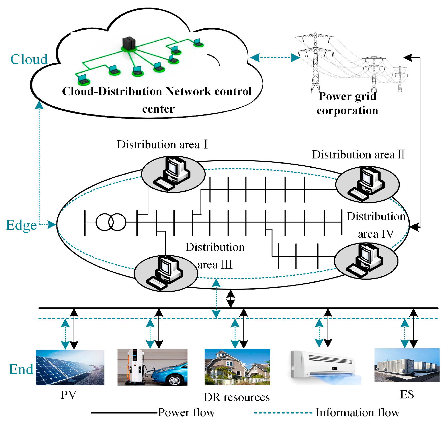
The cloud-edge collaborative scheduling framework for distributed resources in the distribution network is shown in
Figure 1, which specifically includes the following:
(1) The cloud is the scheduling center of the distribution network. It is responsible for the global scheduling of distribution areas and serves as the link for information transmission between distribution areas and the power grid. The main functions of the cloud include collecting and processing the information, performing global dynamic optimization, and then distributing the optimization results to the edge.
(2) Edge is the distribution area, the main gathering area of distributed resources in the distribution network. It can intelligently perceive and aggregate the data uploaded from the end and upload the aggregation results to the cloud. It can also optimize the scheduling instructions issued by the cloud and allocate them to the end. At the same time, information sharing and power exchange can be carried out between edges, thereby achieving efficient and orderly operation of distribution areas.
(3) End is the equipment unit in the distribution area, including distributed new energy, ES devices, and DR resources. It can upload the device’s status information to the edge in real-time and perform the scheduling tasks issued by the edge.
The cloud-edge collaborative scheduling framework of distributed resources in the distribution network constructed in this paper, on the one hand, takes advantage of the resources of the cloud to control the distributed resources in the distribution network globally. On the other hand, taking advantage of the geographical advantage that the edge is close to the data center, the equipment units upload the data information at the end in real-time, analyze it, and process it. At the same time, information transmission is carried out through cloud and edge collaborative interaction, realizing cloud global optimization, cloud-edge collaborative interaction, and edge-end rapid response.
Based on the established collaborative regulation framework of distributed resource cloud edge of distribution network, the equipment units deployed at the end upload the collected equipment state information (including active output, controllable quantity, and cost parameters) and the response information of demand response resources to the edge intelligent distribution terminal of the station area for analysis and processing. The intelligent distribution terminal in the edge area takes real-time data and historical data as inputs, carries out load and photovoltaic data prediction and demand response resource cluster analysis, and then uploads the predicted data and the data after edge aggregation processing to the cloud, and the cloud carries out global data analysis and formulates edge transaction prices, thus realizing bottom-up cloud-edge collaboration. According to the information uploaded by each edge side, the cloud carries out global optimization, formulates the regulation plan of each edge platform area and sends it to the edge, and then formulates the regulation plan of this platform area and sends it to the end-side equipment unit, thus realizing the top-down cloud edge-to-end collaboration.
Under the framework of cloud-side collaborative regulation of distributed resources, the regulation mechanisms of different time scales are as follows:
In the day-ahead stage, the distributed resources in the distribution network are controlled globally. Therefore, with the help of the resource advantages of the cloud, the cloud is taken as the main computing center to carry out global calculation and all DR resources in the distribution network are dynamically optimized globally, and then the task is decomposed to the edge twice. The calculation task of the side is slightly less than that of the cloud, and the calculation task allocated by the cloud is optimized again, and the specific regulation plan is allocated to the end-side DR resources. At this time, only the regulation instructions of the day-ahead DR are issued, and the regulation instructions of the intraday DR and the real-time DR are not issued for the time being, being only used as a reference for the intraday and real-time stages.
- (2)
Intraday stage
Compared with the day-ahead stage, the intraday stage has a slightly shorter time scale. Because all data are uploaded to the cloud center for processing, it will have a great communication delay, so this stage weakens the computing task of the cloud and moves down to the edge. The cloud only collects global data, and sends the task of optimization calculation to the edge, and each edge only carries out independent rolling optimization of intraday DR.
- (3)
Real-time stage
Because the cloud-side collaboration technology uploads the data information on the edge side to the cloud for processing, it will cause serious communication delay and bring great computational pressure to the cloud, prolonging the response time of distributed resources and making it difficult to meet the real-time requirements in the real-time stage. Therefore, compared with the day-ahead and intraday stages, in the real-time stage, this paper moves the computing pressure of the cloud center down, reducing the computing tasks of the cloud, and the cloud only plays the role of auxiliary computing. Instead, it communicates directly with the cloud by means of the end inside the edge, and the cloud sends the decision-making task directly to the end inside each edge. By taking advantage of the proximity of edge computing to the data center, the edge is regarded as an independent optimization area and the information is directly transmitted from end to end, and only the real-time DR is uniformly distributed optimized.
3. Power Scheduling and Deviation Correction Strategy of Three Stages
In this paper, the power deviation problem of distribution network scheduling in different time scales [
21,
22] is solved by gradually refining the time scale, and the power deviation of the distribution network is corrected from three stages: day-ahead, intraday, and real-time. In order to make full use of the response characteristics of distributed resources and make them participate in the multi-time scales scheduling of the distribution network, the response characteristics of DR resources are divided in the time domain, as shown in
Table 1.
According to the division results in
Table 1, the clustering method is used to reduce the dimensionality of distributed resources, and distributed resources with similar response characteristics are clustered into one category. The resource feature extraction and clustering process are detailed in
Appendix A. A three-stage optimization scheduling strategy of distributed resources is proposed based on the distributed resource cloud-edge collaborative scheduling framework. This strategy has formulated corresponding scheduling goals and targets for the scheduling needs of the distribution network at different stages and formulated tasks for cloud and edge under different scheduling stages based on the cloud-edge scheduling framework.
3.1. Day-Ahead Global Optimization Scheduling Strategy
In the day-ahead stage, in order to optimize the overall economic performance of the system, this paper adopts the strategy of all resources participating in the optimization, including day-ahead-type DR, intraday-type DR, real-time-type DR, and ES. At the same time, the power interaction between the distribution areas and between the area and the power grid is also considered. Then, the global dynamic optimization is carried out for each period of the next day. The participation of all resources in the optimization will lead to a large amount of computation. Therefore, based on global optimization, the amount of computation will be allocated to the cloud and edge, and the cloud and edge will undertake different calculation tasks, respectively. The day-ahead stage is divided into the cloud primary and edge secondary optimization. Cloud primary optimization scheduling strategy is shown in
Figure 2.
The initial optimization stage of the cloud is the global optimization stage, and the scheduling object is the distribution area. Firstly, the edge uploads the PV and load prediction values of the day-ahead stage, the declaration information of day-ahead-type DR, the prediction value of intraday and real-time-type DR, and the status information of each device to the cloud. Secondly, each distribution area is regarded as a scheduling unit, and the initial optimization with the cloud is aimed at minimizing the comprehensive operation cost of the distribution network. Formulate the scheduling plans of each distribution area and the power interaction plans between the areas on the next day and release them to the edge. Among them, the price of inter-area power interaction is uniformly set by the cloud, making the distribution area prioritize the inter-area power interaction. When the inter-area power interaction cannot meet the scheduling demand, it will interact with the external power grid, thus promoting collaborative interaction and power support of the distribution areas on the edge.
The second optimization stage is the independent optimization stage, and the scheduling object is the equipment unit in the area. Based on the initial optimization results of the cloud, the second optimization is carried out to minimize the independent scheduling cost of the area, and the optimization results are released to all equipment units in the distribution area. In the secondary optimization, according to the response time characteristics of the intraday-type DR and real-time-type DR, they can participate in day-ahead optimization and intraday and real-time stages optimization, respectively. In order to make full use of the multi-time scale response characteristics of DR resources, only scheduling instructions for the day-ahead-type DR, ES, and interaction with the power grid are issued. The scheduling instructions for intraday- and real-time-type DR are not released and are only for intraday and real-time decision-making.
3.2. Intraday Rolling Optimization Scheduling Strategy
In the intraday stage, based on the global optimization of the day-ahead, power adjustment is carried out for the distributed new energy and load fluctuations, that is, the intraday DR resources and ES scheduling amount, as well as the power interaction amount between the distribution area and the grid, are corrected. Considering the randomness and real-time nature of the intraday DR, to avoid the influence of unplanned power fluctuations on the operation of the distribution area in a short time, a rolling optimization method is adopted in the intraday optimization stage. The distribution area on each edge combines short-term rolling prediction information of PV and load. It makes independent rolling optimization decisions to minimize the cost of correcting the day-ahead deviation. Every 15 min, rolling optimization is conducted to make the scheduling plan for the next 1 h. However, the user is only informed of the scheduling plan for the first 15 min, and the above process is repeated in the next scheduling cycle. The intraday rolling optimization scheduling strategy is shown in
Figure 3.
3.3. Real-Time Consistency Distributed Optimization Scheduling Strategy
In the real-time optimization stage, the prediction accuracy of PV and load is improved further than that in the day-ahead and intraday stages. The real-time stage emphasizes that the distribution network can adjust for unplanned power fluctuations in the ultra-short time scale, so the real-time stage pays more attention to the real-time scheduling ability. In order to reduce the communication delay caused by information transmission, power interaction is no longer carried out between distribution areas. Instead, real-time data on-site analysis and disturbance power nearby processing are carried out in the distribution area near the edge of the data center.
To meet the real-time requirements, this paper uses the fast response speed of real-time-type DR and the fast charging and discharging characteristics of ES equipment to schedule only real-time-type DR and ES in the distribution area [
23]. The real-time consistency distributed optimization scheduling strategy is shown in
Figure 4.
In the real-time stage, according to the latest predicted values of PV and load, ES and real-time-type DR are used as the scheduling units, and the distributed calculation is carried out based on the consensus algorithm to minimize the cost of correcting intraday deviation. When performing consistently distributed computing, only information interaction between adjacent scheduling units within the distribution area is required, so the information transmission amount is small and the optimization convergence speed is fast, which meets the scheduling requirements in the real-time stage [
24]. At the same time, to ensure the global nature of information and the distribution of calculations, a centralized-distributed scheduling method of Leader-Follower is adopted within the distribution area. The Leader obtains the scheduling information of the distribution area from the cloud in real-time and interacts with the neighboring Followers. At the same time, information is transmitted in both directions between neighboring Followers. The schedulable ability determines the selection principle of the Leader [
25]. The real-time DR clusters in the distribution area participate in scheduling for different periods: ES can participate in scheduling all day; therefore, ES is used as the Leader, while the real-time DR cluster is used as the Follower. According to the optimization results of the intraday stage and the latest predicted values of load and PV in the real-time stage uploaded from the edge, the cloud obtains the deviation. It sends it to the Leader of each distribution area. Taking the micro-growth cost rate as the consistency variable, the consistency iteration is carried out for the Leader and Follower of each distribution region. When the micro-increase rate of cost tends to be consistent, the total power command is allocated to each scheduling unit optimally [
26,
27]. In this iteration process, each scheduling unit only needs to exchange information with neighboring units, and the amount of information exchange is small, which can reduce the influence of communication delay. The scheduling instructions in the real-time stage are sent directly to each scheduling unit without going through the user, improving the scheduling efficiency in the real-time stage.
4. Three-Stage Collaborative Optimization Model
This paper builds a three-stage collaborative scheduling optimization model of distribution networks based on the proposed multi-time scale cloud-edge collaborative scheduling strategy, including the day-ahead global optimization scheduling model, intraday rolling optimization scheduling model, and real-time consistency distributed optimal scheduling model.
4.1. Day-Ahead Optimization Scheduling Model
4.1.1. Objective Function
- (1)
Day-ahead initial optimization model
The 24 h scheduling plan for the next day is formulated one day in advance in the day-ahead optimization stage, and the time scale is 1 h. The cloud conducts initial optimization to minimize the comprehensive operation cost of the distribution network. The comprehensive operation cost comprises two parts: the independent scheduling cost of the distribution area and the power interaction cost of the distribution area interval. The objective function can be expressed as Equation (1):
where
is the total scheduling cost of the distribution network in the day-ahead initial optimization;
is the independent scheduling cost of distribution area
in
period;
is the cost of power interaction between distribution area
and other distribution areas; T is the number of periods divided by the day-ahead stage.
The cost of power interaction between distribution areas is shown in Equation (2):
where
and
are the power purchase price and the power sale price of the distribution area interval in the
period, the method for formulating inter distribution area power interaction prices is shown in
Appendix B;
is the power sold by distribution area
to other distribution areas in the
period (kW);
is the power purchased by the distribution area
from other distribution areas in the
period (kW).
- (2)
Day-ahead secondary optimization model
Based on the initial optimization results, secondary optimization is carried out on the edge to minimize the independent scheduling cost of the distribution area. The objective function is expressed as Equation (3):
where
is the total scheduling cost of distribution area
in the day-ahead secondary optimization stage;
is cost of power interaction between the distribution area
and the power grid in the day-ahead stage;
is the operating cost of ES in the day-ahead stage;
is the scheduling cost of the
th cluster of the
load in the distribution area
in the
period;
is the total number of clusters of the
load in distribution area
.
The cost of power interaction between the distribution area and the power grid is shown in Equation (4):
where
and
are the power sold and purchased by the distribution station area
from the power grid during
period (kW);
The operating cost of ES is shown in Equation (5):
where
is the cost coefficient of ES;
is the charging and discharging power of ES (kW), where
indicates that the ES is charging, conversely,
.
The time series power compensation cost model of the DR established in this paper is shown in Equation (6), which considers the influence of response power and response time on decision-making. This model not only provides economic incentives for users in response power but also meets the expected response time requirements of users as much as possible. Users with more response power will get higher economic compensation. When the actual response time of users deviates from the expected response time, they will also be given higher economic compensation.
where
,
, and
respectively represent the time series power compensation cost, power compensation cost, and time compensation cost of the
cluster in the
load in the
period;
represents the load category, with
representing day-ahead-type reducible load, day-ahead-type transferable load, intraday-type reducible load, and real-time directly controlled load;
is the
cluster of the
load;
is the scheduling power of the
cluster of the
load (kW);
and
are the power compensation cost coefficients for the
type of load;
is the unit time compensation cost coefficient of the
load;
and
are the actual response time and expected response time of the
cluster of the
load, respectively.
4.1.2. Constraints
- (1)
Power balance constraint
- (2)
Power interaction constraints in distribution area interval
where
and
are 0–1 variables,
means that distribution area
purchases power from distribution area
, otherwise
;
means that distribution area
sells power to distribution area
, otherwise
.
- (3)
Power interaction constraints between the distribution area and the power grid
where
and
are 0–1 variables, where
means the distribution area
purchases power from the power grid, otherwise
;
means that the distribution area
sells power to the power grid, otherwise
.
- (4)
Charging and discharging constraints of ES
where
and
are the maximum charge and maximum discharge of ES in distribution area
(kW);
and
are 0–1 variables, where
indicates that the ES is in the state of charge, otherwise
;
indicates that the ES is in the state of discharge, otherwise
;
and
are respectively the state of charge of the ES in the distribution area
in the
period and in the
period;
and
are the upper and lower limits of the state of charge of ES (%);
and
are the charging and discharging efficiency of ES;
and
are the initial and final state of charge of ES in a scheduling cycle (%).
- (5)
The constraint of DR
where
is the maximum schedulable power reflected by the centroid of the
cluster in the
load (kW).
4.2. Intraday Optimization Scheduling Model
4.2.1. Constraints
Based on the day-ahead optimization results, the intraday optimization adjusts the day-ahead scheduling plan by rolling optimization based on the latest predicted intraday PV and load values. Intraday optimization takes 1 h as a rolling cycle, and the 1 h scheduling plan is formulated 15 min in advance. However, only the first 15 min of scheduling results are performed, and the next 15 min repeat the above process. The goal is to minimize the cost of correcting the day-ahead deviation in the distribution area, and its objective function can be expressed as (13):
where
is the scheduling cost of distribution area
in a scheduling period of intraday stage;
is the cost of power interaction between the distribution area
and the power grid in the intraday stage;
is the operating cost of ES in the intraday stage;
is the scheduling time-scale of intraday stage; M is the number of scheduling periods included in an intraday scheduling stage.
4.2.2. Constraints
- (1)
Power balance constraint
- (2)
The power interaction constraints between the distribution area and the power grid, the charging and discharging constraints of ES, and the constraint of DR are similar to the day-ahead stage, which is no longer described here.
4.3. Real-Time Optimization Scheduling Model
The goal of the real-time stage is to minimize the cost of correcting intraday deviation in the distribution area, and its objective function can be expressed as Equation (15):
where
is the scheduling cost of distribution area
in the real-time stage;
is the scheduling cost of the
cluster of real-time-type DR in the distribution area
;
is the scheduling cost of ES in distribution area
.
According to the criterion of equal micro-increase rate of cost, when the micro-increase rate of cost of all scheduling units tends to be consistent, the total scheduling cost of the distribution area is the smallest, so as to realize the optimal distribution of the scheduling power among the scheduling units. Therefore, in the real-time stage, the time scale is 5 min. Of course, it is also applicable to take a shorter time in practical application. The micro-increase rate of the scheduling cost of each scheduling unit in the real-time stage is used as the consistency variable, and the distributed calculation is carried out based on the consistency algorithm.
In the process of optimizing calculations using consensus algorithms, each scheduling unit is regarded as a node. For node
,
represents the consistency status information of node
after
iterations, where
The consistency variables of each node are updated according to the consistency variables of its adjacent nodes. With the gradual increase in the number of iterations, the consistency variables
of any adjacent nodes tend to be consistent. When
is satisfied, all nodes in the system are considered to converge to the common value. We define matrix
as the adjacency matrix, whose diagonal element is 0, and the non-diagonal element
is the number of edges from node
to node
.
is the state transition matrix; if the matrix
is a non-negative row random matrix and all eigenvalues are not greater than 1, all scheduling units in the distribution area will converge to the same value after enough iterative operations.
is the Laplace matrix, which reflects the topological structure of the scheduling units in the distribution area and satisfies the relationship shown in Equation (16):
where
is the element of row
and column
of
which is determined by the communication network topology and can be expressed as Equation (17):
where
is the gain weight from node
to node
;
is the element in row
and column
of
.
The micro-increase rate of cost is defined as the derivative of the scheduling cost to the scheduling power, so the micro-increase rate of cost of ES and real-time-type DR can be expressed as Equation (18):
where
is the micro-increase rate of cost of the scheduling unit
in the distribution area
in the
period.
In this paper, ES is selected as the Leader, and the cluster of real-time-type DR is selected as the Follower. The micro-increase rate of cost of
iterations of Leader can be expressed as Equation (19):
where
is the power scheduling coefficient;
is the total power deviation of distribution area
in the
period;
is the residual deviation after scheduling.
The micro-increase rate of cost of
iterations of Follower can be expressed as Equation (21):
According to Equations (5), (6) and (18), the scheduling power of
iterations in the
period can be obtained. The scheduling power of Leader can be expressed as shown in Equation (22).
The scheduling power of Follower can be expressed as follows:
where
is the scheduling power of the scheduling unit
in distribution area
after
iterations in the
period (kW), and
and
are the upper and lower limits of the scheduling power of the scheduling unit
(kW).
In the iterative calculation process of the consensus algorithm, the residual deviation
is used as the convergence condition. When
, the consistency calculation reaches convergence, and
is the convergence error. Iteratively update
, until all
tends to the same value
, at which point the system reaches a consistent convergence, that is, the micro-increase rate of cost of all scheduling units in the distribution area is consistent.
The optimal values of the scheduling power of the ES and the real-time-type DR cluster are shown in Equations (26) and (27), respectively:
4.4. Solution Method
The multi-time scale cloud edge optimization and regulation model of distribution network belongs to a nonlinear programming problem, so MATLAB combined with yalmip plug-in is used to call gurobi solver to solve it in the days before and during the day. In the real-time stage, in order to ensure its real-time control ability, MATLAB is used for distributed calculation based on consistency algorithm. The specific algorithm flow is shown in the following
Figure 5.
The specific solution steps are as follows:
Step 1, the edge side platform area uploads the load, the day-ahead forecast information of photovoltaic, and the parameter information of each control unit to the cloud;
Step 2, the cloud carries out global initial optimization a few days ago with the goal of minimizing the comprehensive operation cost of the distribution network, and sends the optimization result to the edge platform area;
Step 3, each edge platform area carries out the second optimization decision day-ahead with the minimum cost of independent regulation and control of the platform area as the goal and sends the optimization result to the regulation and control unit in the previous stage;
Step 4, the edge updates the intra-day forecast information of load and photovoltaic;
Step 5, the edge platform area carries out intra-day rolling optimization with the goal of minimizing the deviation cost before the correction day and sends the optimization result to the intra-day stage adjustable unit;
Step 6, the real-time forecasting information of load and photovoltaic is updated in the platform area on the edge;
Step 7, the Leader of each area obtains the power deviation to be corrected in the station area and calculates the slight increase rate of the cost of each control unit;
Step 8, a Laplacian matrix and a state transition matrix are formed according to the topological structure inside each station area;
Step 9, the consistency variables of Leader and Follower and the regulating power are updated according to Formulas (22) and (23), respectively;
Step 10, judging whether the current iteration result meets the convergence condition, and if not, performing the next iteration; if the conditions are met, the final optimization result is output.
5. Example Analysis
The effectiveness of the strategy proposed in this paper is verified by taking a regional distribution network as an example. Multi-time scale cloud-edge collaborative distribution network optimization is a nonlinear programming problem. Based on the results of the above solution, the time-of-use power price of the power grid refers to
Table A1 in
Appendix C; the parameters of ES refer to
Table A2 in
Appendix C; the parameters of DR resources are shown in
Table A3 in
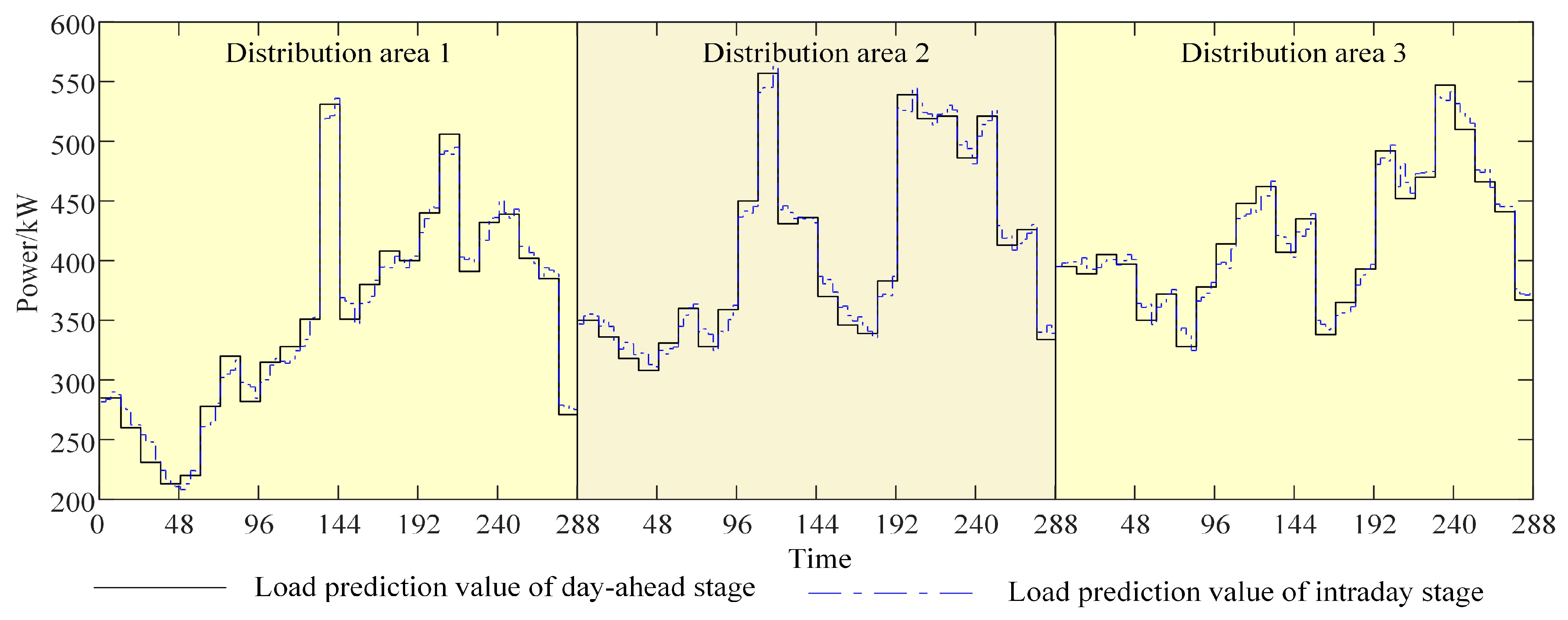
Appendix C. In addition, the load and PV forecast curves are shown in
Figure A1 and
Figure A2 in
Appendix C.
5.1. Analysis of Clustering Results
According to the response information of the DR declared by users, the improved K-means clustering analysis method is used to aggregate the day-ahead-type reducible loads, day-ahead-type transferable loads, intraday-type reducible loads, and real-time-type directly controlled loads into a certain number of resource clusters. The internal resources of each cluster have similar characteristics of power consumption. Among them, the schedulable duration of declaration of day-ahead-type reducible loads and day-ahead-type transferable loads is ; the schedulable duration of intraday-type reducible loads is ; the schedulable duration of real-time-type directly controlled loads is ; the number of controllable resources declared by the four loads is 100; where represents uniform distribution between and .
The optimal number of clusters for DR is shown in
Table S1, and the clustering results are shown in
Tables S2. The centroid in each cluster represents the power consumption behavior characteristics of the users in the corresponding cluster, the time to enter the distribution network, the time to leave the distribution network, the expected response time, and the maximum reducible power of each cluster body is reflected by the centroid. The centroid feature represents the response characteristics of all resources within the cluster, which can be used to uniformly schedule the resources within the cluster according to the centroid feature.
5.2. Analysis of Optimization Results
In order to verify the effectiveness of the strategy proposed in this paper, we analyze the optimization results of the distribution network cloud-edge framework in three stages: day-ahead, intraday, and real-time.
5.2.1. Analysis of Day-Ahead Optimization Results
In order to facilitate the analysis of the day-ahead optimization results, the day-ahead initial optimization results and the day-ahead secondary optimization results of the distribution area are shown in the exact figure, as shown in
Figure 6.
Figure 6a–c shows the optimization results in the day-ahead stage of three distribution areas. In addition, the optimized scheduling results for each DR cluster are shown in
Figures S1–S4.
As shown in
Figure 6, it can be seen that all distribution areas have similarities in scheduling plans for DR and ES and power interaction plans of distribution area intervals. There is no PV in all distribution areas at 0:00~5:00 and 19:00~24:00, so the load demand is mainly met by purchasing a large amount of power from the power grid. At the same time, the power purchase price from the power grid at this period is low, so the ES will be charged to facilitate the discharge during the peak period of power price. At 19:00~22:00, the load demand of all areas is high, and there is no PV. Therefore, the load demand is met by purchasing power from the power grid, scheduling DR, and discharging the ES. At 11:00~15:00, the PV output is greater than the load demand in Distribution Area 2, while the PV output cannot meet the load demand during this period in Distribution Area 1 and Distribution Area 3. Distribution Area 2 will prioritize the sale of excess renewable energy supply to Distribution Area 1 and Distribution Area 3 with power shortage to realize the local utilization of resources. In addition, the remaining power is sold to the grid.
For DR resources, the day-ahead-type transferable loads can transfer the loads at the peak price to the period of low price, which has a good economy. The day-ahead-type reducible loads scheduling period users declare is mainly during the daytime. Since the price of power purchased from the power grid is high in the daytime, it is more economical to maintain the power balance by reducing the load. For intraday-type DR and real-time-type DR, due to their fast response speed and relatively high compensation price, the distribution area preferentially schedules the day-ahead-type DR. It formulates the scheduling plan of intraday-type DR and real-time-type DR as a reference for the intraday and real-time scheduling stage, but does not release them.
Through the optimization results of the clusters shown in
Figures S1–S4, it can be seen that all clusters consider the constraints of response time and response quantity when participating in scheduling, thus ensuring that the scheduling instructions respond within the constraint range in the day-ahead stage.
5.2.2. Analysis of Intraday Optimization Results
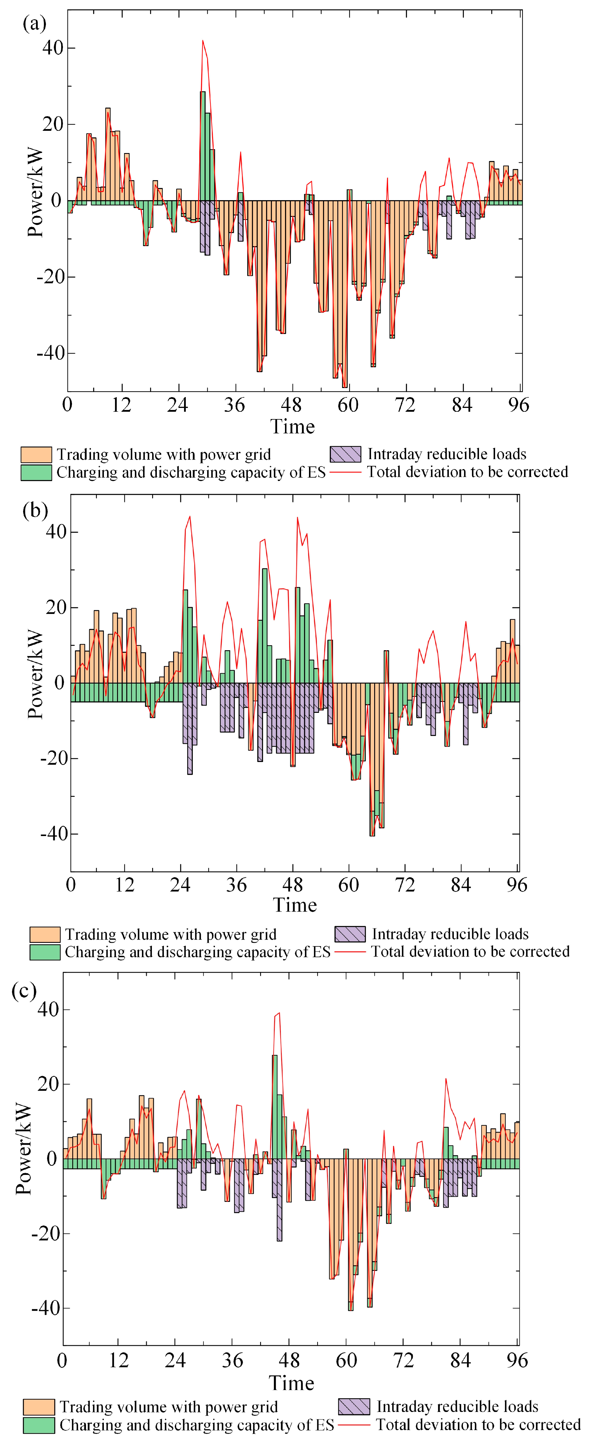
The intraday stage scheduling plan takes the day-ahead scheduling results as the baseline for rolling optimization. It adjusts the power interaction between the distribution area and the power grid, the charging and discharging capacity of ES, and the scheduling of intraday-type DR. As shown in
Figure S1, the power deviation needs to be corrected in the distribution area during the intraday. The difference between load and PV deviations is the total deviation to be corrected. The deviation is positive if the PV and load predicted values of the intraday stage are greater than those of the previous day stage. If predicted values of PV and load in the intraday stage are smaller than those in the previous day, then the deviation is negative.
Deviation correction is carried out in the intraday stage, and the optimization results are shown in
Figure 7. The scheduling results of each cluster of intraday-type reducible load are shown in
Figure S5.
According to
Figure 7, when the total power deviation is greater than 0, the power balance can be achieved by discharging ES, scheduling intraday-type DR, and purchasing power from the power grid. When the total power deviation is less than 0, the power balance can be met by charging ES and selling power to the power grid. Moreover, the intraday scheduling plan makes power adjustments based on the day-ahead plan, which ensures a compelling connection between the day-ahead global optimization and the intra-day rolling optimization.
It can be seen from the scheduling results of intraday-type reducible loads in
Figure S5 that each cluster responds to the scheduling instructions in the intraday stage within the range of meeting the response time constraints and response amount constraints. Moreover, the scheduling power of each cluster also effectively refers to the scheduling instructions optimized in the day-ahead stage.
5.2.3. Analysis of Real-Time Optimization Results
In real-time stage, based on the results of intraday scheduling, the real-time power scheduling simulation analysis of the distribution area is carried out on the time-scale of 5 min. The power adjustment coefficient of the consensus algorithm is
, and the convergence error is
. As show in
Figure S2, the power deviation needs to be corrected in the real-time stage.
Shown in
Figure 8 is the communication topology diagram of the real-time scheduling units in the distribution area 1. Taking the power deviation
kW that needs to be corrected at 7:05 as an example, the real-time stage simulation is carried out. According to the response information of each real-time-type DR cluster, it can be seen that a total of six clusters (cluster 4, 6, 9, 10, 14, 15) and ES participate in the scheduling of distribution area 1.
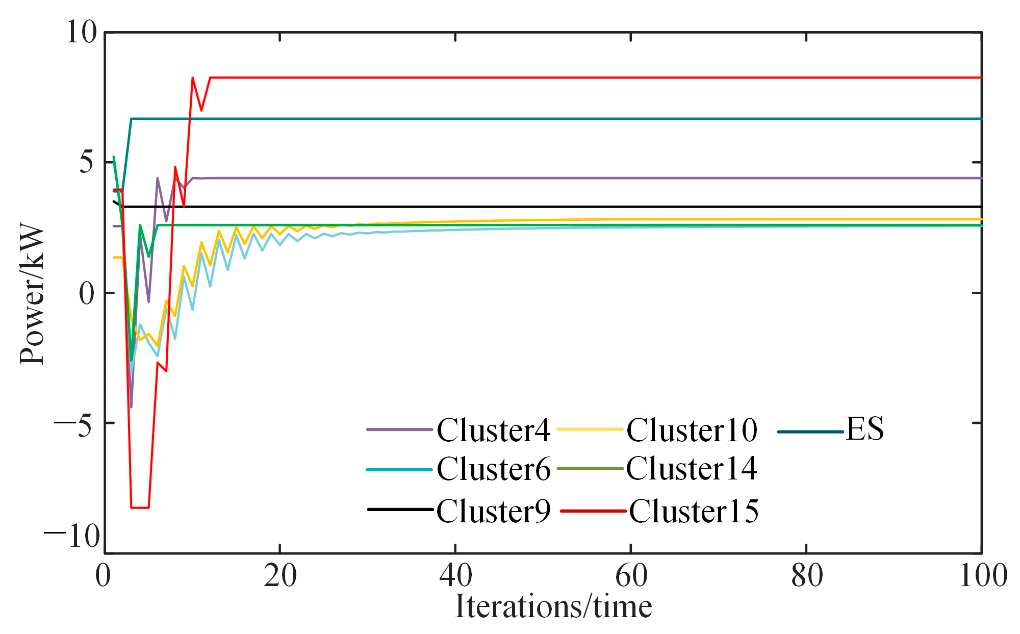
Shown in
Figure 9 is the consistent convergence process of the micro-increase rate of cost of scheduling units in the real-time stage;
Figure 10 shows the convergence process of the scheduling power of scheduling units in the real-time stage.
The analysis of
Figure 9 shows that the micro-increased cost rate of the scheduling unit is different at the initial time. The micro-increase rates of cost of ES and cluster 4 increase first and then decrease, and finally tend to be unchanged. The micro-increase cost rates of clusters 6, 9, 10, 14, and 15 gradually increase and eventually tends to remain unchanged. The cost micro-increase rate of all scheduling units reached a consistent convergence when iterating 35 times, which is 0.2618 CNY/kWh.
When the micro-increase rate of cost tends to be consistent, the optimal scheduling power values of all scheduling units are
=
kW,
=
kW,
=
kW,
=
kW,
kW,
kW, and
kW, as shown in
Figure 10, and the scheduling results of all scheduling units are within the operating constraints.
5.3. Comparative Analysis of Different Scenarios
5.3.1. Comparative Analysis of Three Stages
To verify the effectiveness and economy of the scheduling strategy proposed in the three stages of day-ahead, intraday, and real-time in this paper, the following four example scenarios are set up for comparative analysis.
Scenario 1: Each distribution area operates independently. The traditional centralized optimization is used to formulate the scheduling plan, and DR is not considered in the three stages.
Scenario 2: Based on the distributed resource cloud-side collaborative framework proposed in this paper, the scheduling is carried out, but DR is not considered in the three stages.
Scenario 3: Each distribution area operates independently. In the three stages, the traditional centralized optimization is used to formulate the control plan, and the multi-time scale characteristics of DR are considered to participate in the scheduling.
Scenario 4: The three-stage cloud-edge collaborative scheduling strategy of distributed resources proposed in this paper is used to optimize.
According to the above scenarios, the scheduling costs in four scenarios are obtained through optimization calculation, as shown in
Table 2.
As shown in
Table 2, the scheduling cost under scenario 2 is lower than in scenario 1 by 3.61%. Scenario 1 and scenario 2 do not consider DR. The difference is that scenario 1 adopts the traditional centralized optimization scheduling method, and all distribution areas operate independently. When the resources in the distribution area cannot meet the power balance, they can only buy and sell power from the power grid. In scenario 2, the multi-time scale scheduling strategy under the cloud-side collaborative framework is applied, the scheduling power is reasonably distributed on the cloud and edge, and the power interaction between distribution areas is considered. When the power supply in the distribution area is insufficient, the priority should be given to purchasing power from the distribution area with surplus power instead of directly purchasing power from the power grid to reduce the cost of purchasing power. When the power supply in the distribution area is surplus, it is preferentially sold to the area with a power shortage and then selected to be sold to the power grid, thus improving the power sales revenue. Compared with scenario 3, the scheduling cost of scenario 4 is reduced by 6.80%. In addition, scenario 3 and scenario 4 consider the response time characteristics of DR so that DR resources can participate in multi-time scale scheduling according to their different response time characteristics. However, the scheduling cost of scenario 4 is lower than that of scenario 3, because scenario 4 adopts a multi-time scale cloud-edge cooperative scheduling strategy. In contrast, scenario 3 adopts a traditional centralized optimization control method, similar to scenarios 1 and 2 above. Cloud-edge collaborative optimization control can improve the economy of the overall operation of the system.
Compared with scenario 1, the scheduling cost of scenario 3 is reduced by 12.43%; both scenarios adopt the traditional centralized optimization scheduling method. The difference is that scenario 3 considers DR resources with different response time characteristics, while scenario 1 does not consider this. Compared with scenario 2, the scheduling cost of scenario 4 is reduced by 15.33%; both scenarios adopt the multi-time scale scheduling strategy of cloud-edge coordination, but scenario 4 also considers the multi-time scale characteristics of DR resources and makes them participate in scheduling. It can be seen that DR participates in the scheduling to improve the flexibility of distribution network operation. Under the premise of the optimal economy of the distribution network, the purchasing of power is reduced through the scheduling of DR resources, and the sales of power are increased to obtain more benefits. The analysis shows that the economy of distribution network operation can be improved by adding DR.
Through the analysis of the scheduling costs of the four scenarios, it can be seen that the economic efficiency of distribution network operation can be improved whether considering the cloud-edge collaborative optimization scheduling or considering the multi-time scale characteristics of DR, thus verifying that the scheduling strategy proposed in this paper has good economic benefits. However, due to the small number of distribution areas considered in this paper, the effect on improving the economy is limited. For the distribution network with more distribution areas, under the cloud-edge framework, the power interaction and DR resources of the edge areas will play an important role in the scheduling. They will have a significant effect in improving the operation economy of the distribution network. Therefore, the research results of this paper provide an essential reference for the scheduling of distribution networks composed of multiple distribution areas in the future.
5.3.2. Comparative Analysis of Real-Time Stage
In order to verify the effectiveness of the proposed scheduling method in the real-time stage, the following two scenarios are set for comparative analysis.
Scenario1: Centralized computing is performed by the cloud center, and then the scheduling tasks are released to the scheduling units.
Scenario 2: The centralized-distributed calculation based on the consensus algorithm is adopted, and the adjacent scheduling units perform information interaction.
It can be seen from
Table 3 that the convergence time of centralized scheduling is significantly larger than that of centralized-distributed scheduling because the data information of all scheduling units of centralized control must be uploaded to the cloud center for unified calculation, thus increasing the time of data transmission and processing. In scenario 2, centralized-distributed computing based on a consensus algorithm only requires information interaction between adjacent scheduling units, significantly reducing the amount of calculation. Therefore, scenario 2 has a faster optimization speed than scenario 1. With the increase in the scale of the distribution area, the advantages of distributed optimization calculation will be more prominent, which is more in line with the real-time scheduling requirements in the real-time stage.
6. Conclusions
This paper considers the spatial and temporal characteristics of DR resources and proposes a three-stage cloud-edge collaborative optimization control strategy for distributed resources. Through example analysis, the following conclusions can be drawn:
(1) In the day-ahead stage, the power interaction and sharing between the distribution areas on the edge have been considered, fully leveraging the advantages of collaborative scheduling on the edge. Through the power interaction between areas, the local consumption of resources has been achieved, and the overall economic operation of the distribution network has also been improved.
(2) It adapts to the change of PV and load forecasting accuracy through the coordinated scheduling of three-time scales of day-ahead, intraday, and real-time in the cloud and edge. Considering the response time characteristics of DR, participating in the optimal scheduling of the distribution network fully taps the scheduling potential of DR, improves the flexibility of power flow between distribution areas, and significantly improves the economy of distribution network operation.
(3) In the real-time stage, the centralized-distributed calculation is carried out based on the consensus algorithm, and the micro-increased cost rate of the scheduling unit is selected as the consistency variable. When the micro-increase rate of cost tends to be consistent, the optimal allocation of the scheduling power of each scheduling unit in the distribution area can be realized. Compared with centralized calculation, it can reduce the calculation time and improve the optimization speed.
The regulation strategy proposed in this paper is suitable for small-scale distribution systems. For large-scale power systems, with the increase in the type and quantity of DR resources on the load side and the complexity of user uncertainties, it will be more difficult to coordinate and optimize the regulation strategy between the power grid and users. Therefore, in future research, it will be necessary to consider more complex and larger power grid environments and study multi-objective optimization regulation strategies.


