
Power System Transient Stability Preventive Control via Aptenodytes Forsteri Optimization with an Improved Transient Stability Assessment Model


1
Department of Electrical and Power Engineering, Taiyuan University of Technology, Taiyuan 030024, China
2
Department of Electrical Engineering and Applied Electronic Technology, Tsinghua University, Beijing 100084, China
3
China Electric Power Research Institute, Beijing 100192, China
*
Author to whom correspondence should be addressed.
Energies 2024, 17(8), 1942; https://doi.org/10.3390/en17081942
Submission received: 18 March 2024
/
Revised: 15 April 2024
/
Accepted: 17 April 2024
/
Published: 19 April 2024
(This article belongs to the Section F: Electrical Engineering)
Abstract
:Transient stability preventive control (TSPC), a method to efficiently withstand the severe contingencies in a power system, is mathematically a transient stability constrained optimal power flow (TSC-OPF) issue, attempting to maintain the economical and secure dispatch of a power system via generation rescheduling. The traditional TSC-OPF issue incorporated with differential-algebraic equations (DAE) is time consumption and difficult to solve. Therefore, this paper proposes a new TSPC method driven by a naturally inspired optimization algorithm integrated with transient stability assessment. To avoid solving complex DAE, the stacking ensemble multilayer perceptron (SEMLP) is used in this research as a transient stability assessment (TSA) model and integrated into the optimization algorithm to replace transient stability constraints. Therefore, less time is spent on challenging calculations. Simultaneously, sensitivity analysis (SA) based on this TSA model determines the adjustment direction of the controllable generators set. The results of this SA can be utilized as prior knowledge for subsequent optimization algorithms, thus further reducing the time consumption process. In addition, a naturally inspired algorithm, Aptenodytes Forsteri Optimization (AFO), is introduced to find the best operating point with a near-optimal operational cost while ensuring power system stability. The accuracy and effectiveness of the method are verified on the IEEE 39-bus system and the IEEE 300-bus system. After the implementation of the proposed TSPC method, both systems can ensure transient stability under a given contingency. The test experiment using AFO driven by SEMLP and SA on the IEEE 39-bus system is completed in about 35 s, which is one-tenth of the time required by the time domain simulation method.
1. Introduction
With the increase in penetration of renewable energy and the widespread application of novel power electronic devices, the complexity and uncertainty of modern power systems have increased significantly. As a result, the systems gradually operate close to security stability limits [1,2,3]. Preventive control strategies for power systems are designed to adjust the system to a reliable operating point before probable contingencies occur. Formulating effective grid operation points and stability control strategies involves comprehensive simulation analysis. This process needs to be enhanced due to its inherently time consumption nature. Therefore, research on the development of a rapid transient stability preventive control strategy is of utmost importance to guarantee the transient stability of power systems.
Transient stability assessment (TSA) is a methodology for evaluating the transient stability state of a power system by analyzing system operational features. The traditional transient stability assessment methods contain the time domain simulation method [4] based on large-scale simulation calculations and the direct method [5] based on Lyapunov’s stability theory. The accuracy of these conventional methods is undeniable. However, their innate complexity often leads to a considerably long process of obtaining swift stability results. Data-driven TSA is becoming increasingly popular in academia and industry because traditional time-domain simulations and the direct method cannot match the real operation requirements of power systems [6,7]. Machine learning methods [8,9], involving widely used data feature mining algorithms, possess the capability of establishing a mapping relationship between input features and output. A TSA model can be built by machine learning algorithms, where the operational features of the system are taken as the input, and the assessment of transient stability is taken as the output. In [10], a series of location-specific decision tree (DT) regressors are trained for TSA, which leads to an improvement in the stability margin at specific locations. An imbalanced correction method based on a support vector machine (SVM) is proposed in [11], and this method is used to establish the TSA model. In [12], the extreme gradient boosting (XGBoost) algorithm is introduced to recognize different unstable patterns after a power system fault. The aforementioned studies aim to develop TSA models using machine learning algorithms. However, due to the simplicity of the model’s structure, the accuracy of the above TSA models is insufficient. Moreover, the use of a black box model in these approaches limits the interpretability of the results. Compared with traditional machine learning methods, deep learning methods [13,14], which use multiple layers to progressively extract higher-level features from the raw input, have the advantages of strong feature extraction ability and good convergence. In recent years, deep learning algorithms have been widely applied to TSA in power systems. For instance, in [15], an improved Deep Belief Network (DBN) model is proposed for the rapid assessment of transient stability, along with a reasonable interpretation of the underlying relationship between system features and assessment results. Additionally, reference [16] proposes a transient stability predictor that considers operational variability based on a Convolutional Neural Network (CNN) ensemble method, to enable adaptation to near-future operation conditions in a limited time. Moreover, using the latest deep learning techniques such as Generative Adversarial Networks (GAN) [17] for online TSA is explored. Notably, although these studies constructed TSA models with higher accuracy using deep learning techniques, they did not guide the development of system control strategies. Therefore, further research efforts should aim to leverage these high-accuracy models in developing effective control strategies for power systems.
Transient stability preventive control (TSPC) aims to withstand high-probability severe contingencies through measures such as generation rescheduling [18]. However, system generation rescheduling can result in substantial dispatching costs, which can be onerous for system operators. To resolve this conflict between economy and stability requirements, transient stability constraints are introduced into optimal flow formulation. The presence of transient stability constraints manifested as differential-algebraic equations (DAE) [19] poses a significant challenge to conventional optimization algorithms. Specifically, the DAE’s complexity makes it difficult to apply standard mathematical optimization methods. Linear programming and the interior point method are utilized in [20] and [21], respectively. These approaches use advanced mathematical optimization algorithms to overcome the limitations of DAE but still suffer from significant time consumption. In reference [22], the application of a Backpropagation Neural Network (BPNN) optimized through the genetic algorithm (GA) is employed as the TSA model. This approach is further enhanced by integrating it with the particle swarm algorithm to assess the power system’s transient stability after conducting TSPC strategies. Nevertheless, this approach just uses a basic BPNN structure, is unreliable in evaluation outcomes, and is inappropriate for complex scenarios. In ref. [23], DBN is strategically integrated with a non-dominated sorting genetic algorithm (NSGA-III) to develop a new preventive control framework. This method reduces the difficulty of solving DAE by replacing them with TSA. However, the optimization solution path of NSAG-II is single, and the method described in the paper lacks the necessary prior knowledge to assist in the rapid optimization solution.
In summary, the drawbacks of the existing studies can be summarized as follows:
- The traditional TSC-OPF issue incorporated with differential-algebraic equations (DAE) is time consumption and difficult to solve.
- Due to the simplicity of the machine learning model’s structure, the accuracy of TSA models is insufficient. The common deep learning approach has three drawbacks: it only has one input feature set, it is difficult to choose structures, and its assessment results’ dependability is unknown.
- When TSA is directly introduced into the OPF as a constraint, the issue of lack of prior knowledge will arise. As a result, features that have little effect are frequently added as input features to the optimization process, which lowers the efficiency of optimization.
- Widely used optimization algorithms often have only one optimization path. This can lead to algorithms that are not fast enough to solve, and the accuracy of the results needs to be improved.
In response to the many problems in the above studies. This paper proposed a novel TSPC method driven by naturally inspired optimization with improved transient stability assessment. The main contributions of this paper are as follows:
- In this paper, an ensemble learning model is used as a TSA model to solve the DAE equation, which simplifies the calculation and improves the efficiency.
- The stacking ensemble multilayer perceptron (SEMLP) approach is introduced to determine the transient stability of the system. The two-layer integrated model is designed in this paper to extract valuable information from diverse system operational features, thereby enhancing the overall model’s generalizability and accuracy. Based on this method, an online TSA model is developed and serves to determine the transient stability for TSPC.
- Sensitivity analysis based on TSA is used to determine the adjusting direction of the controllable generator set. The results of the sensitivity analysis are input as a priori knowledge into the subsequent optimization algorithm to improve the efficiency of the optimization algorithm.
- A novel TSPC method, AFO driven by SEMLP, is introduced to achieve a good balance between stability, economy, and rapidity in generation rescheduling.
2. Transient Stability Assessment Model Based on SEMLP
2.1. Stacking Ensemble Multilayer Perceptron
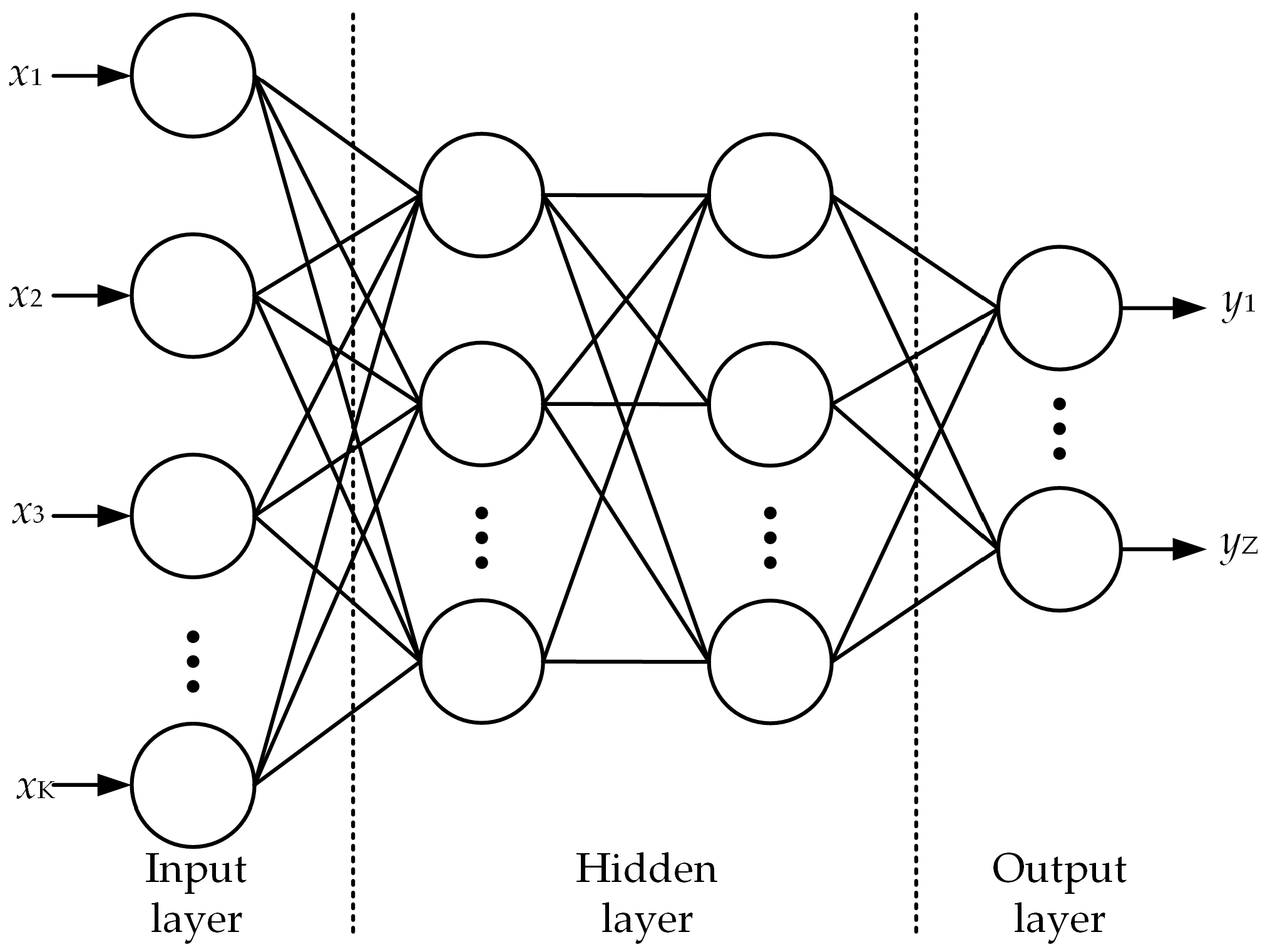
Multilayer perceptron (MLP) is a quintessential deep learning algorithm, which consists of several fully connected perceptron layers interconnected through an extensive neural network architecture. The structure of MLP is shown in Figure 1. The last layer uses the softmax function as the activation function to output the labels for classification and recognition, and the remaining intermediate layers perform feature extraction layer by layer.
Despite its powerful feature extraction capabilities, optimizing only one single MLP model to find the optimal settings can be a time consumption and labor-intensive process.
Stacking ensemble learning [24,25] combines multiple learning algorithms to improve the model’s accuracy. It involves training multiple weak classifiers and then combining them to create a stronger classifier. The general idea is to use a meta-learner to learn from the outputs of the basic classifiers. The meta-learner then makes a final decision. Figure 2 shows the basic structural diagram of stacking ensemble learning.
The stacking ensemble learning approach can be employed to mitigate the influence of variable parameters in MLP classifiers and enhance their accuracy. By combining multiple MLP models trained on different data sets, the SEMLP method can help alleviate the overfitting problem and improve the generalization ability of the model. As a result, it can outperform a single MLP model in terms of accuracy and efficiency.
2.2. Input Vectors and Output of SEMLP
The TSA model is trained with diverse factors that affect the stability of the power system, including generators’ output and bus features. These factors are critical in assessing the power system’s transient stability during disturbances. By incorporating these diverse factors within the TSA model, it becomes more effective in identifying potential stability issues and providing preventative measures. In this research, three types of feature data are introduced for use in TSA. The first feature set (PG1, PG2, …, PGn) refers to the generators’ active power output, the second feature set (|V1|, |V2|, …, |Vn|) refers to bus voltage magnitudes, and the third feature set refers to bus voltage angle difference. m represents the total quantity of buses. n denotes the total number of generators. Therefore, the input to SEMLP is as follows:
The Transient Stability Index (TSI) is used as a quantitative measure to evaluate the transient stability of a system. TSI is an indicator that quantifies the maximum deviation in rotor angle among the power system’s generators throughout the transient period. The TSI formula is presented as follows:
is the largest difference in rotor angle between any two generators. TSI 0 reflects that the power system is in a state of transient stability, whereas TSI 0 indicates that the power system is in a state of transient instability. The numerical simulation samples’ TSIs are all determined using PSASP. In this research, the TSA model is employed to replace the nonlinear DAEs, which are conventionally used to impose transient stability constraints. The SEMLP model accurately establishes the connection between diverse system operational features and TSI values. Therefore, the output of SEMLP is as follows:
2.3. Training of the TSA Model Based on SEMLP
The structure of the TSA model based on SEMLP is shown in Figure 3.
The specific steps for training SEMLP are as follows:
Step 1. Input the time-domain simulated sample data into the model. As shown in Figure 3, Feature A is inputted into MLP-1, MLP-2, and MLP-3. Feature B is inputted into MLP-4, MLP-5, and MLP-6. Feature C is inputted into MLP-7, MLP-8, and MLP-9.
Step 2. By training MLPs with different structures in parallel, the basic classifier layer is built up. The specific neural network parameters of the SEMLP model are shown in Table 1. As Table 1 shows, each MLP sub-model possesses its unique architecture.
These sub-models are utilized to construct a base classifier layer, with each MLP independently processing a specific set of features. The outputs of the three MLP sub-models corresponding to each feature are then integrated through a process of averaging. TSI-pre integration, the three mean values, are considered as the output of the basic classifier layer. This integrated approach ensures that each sub-model’s contribution is given equal weight, effectively combining the results in a balanced and comprehensive manner.
Step 3. Train the meta-classifier layer. The actual TSI label that corresponds to the feature set is used as the input label for the meta-classifier, while the output of each base classifier is used as the input feature for the meta-classifier. This research uses a weighted cross-entropy loss function to solve the imbalance between the number of stable samples and the number of unstable samples. The specific weighting process is described as follows:
where L means the calculation of the cross-entropy loss function; Nsp donates the total number of samples; yi represents the real stability label of the i-th sample, and the value of yi is 0 or 1; represents the probability that the predicted label of the i-th sample is stable, and ; Ws and Wu are loss weights for stable and unstable samples, respectively. To draw more emphasis to the unstable sample with very small sample sizes, we set Ws < Wu.
Step 4. Obtain the predicted results of TSA. The SEMLP model’s output is the TSI predicted value. TSI < 0 indicates that the power system is in a state of transient instability. The suggested SEMLP method and TSI index can not only assess binary information regarding the samples’ state but also calculate the stability margin or instability degree.
2.4. Evaluation Indices
Table 2 displays the TSA evaluation results.
TSA is a non-equilibrium classification problem. This research has adopted the evaluation indices: Acc, TPR, TNR, and Gmean. Acc is the overall classification accuracy. TPR means the ability to identify stable samples. TNR denotes the ability to identify unstable samples. Gmean is a comprehensive index.
2.5. Controllable Generator Set Selection Based on Sensitivity Analysis
To enhance the effectiveness of the solution of the optimization, it is crucial to find the generators that have a significant influence on transient stability. The trajectory sensitivity can be computed using the pre-trained neural network parameters, which can then be utilized to form positively and negatively adjusted generator sequences.
For a regular neural network, the output of the fully connected layer can be expressed as follows:
where xnm represents the input from the n-th to the m-th layer; and bnm represent the weights and biases, respectively; σ is the activation function; Mn is the number of neurons per layer. Rewrite (9) in the form of a mapping relation:
where I represents the initial input vector to SEMLP. The derivative function of fn can be expressed as:
Therefore, the partial derivative of output with respect to input can be expressed as follows:
This partial derivative can be used as the sensitivity of controllable generators:
where is the sensitivity of the i-th controllable generator’s active power with respect to TSI.
Depending on , all generators in the power system can be divided into positively adjusted generator sequences and negatively adjusted generator sequences.
where and represent the k-th controllable generator in and , respectively. Generators in positively adjusted generator sequence are sorted by the size of the adjustment amount from largest to smallest. Reversely, generators in negatively adjusted generator sequence are sorted from smallest to largest. The positive and negative adjustment sorts can be incorporated into the initial sample set as prior knowledge for the subsequent optimization algorithm.
3. Transient Stability Preventive Control Algorithm
TSPC encompasses control measures taken to guarantee the stability of the system during normal operation, involving aspects such as generator output control, load control, voltage control, etc. TSPC can be considered equivalent to transient stability-constrained optimal power flow (TSCOPF). TSCOPF seeks to optimize the power system’s parameters while adhering to certain safety limits, thereby facilitating reliable operation even in the face of external perturbations.
3.1. TSCOPF
3.1.1. Objective Function
The TSPC strategy employs generator output control as the primary method, and the optimization objective is to minimize the total cost of adjustment:
where C represents the total cost of the controllable generator set’s output adjustment; SG denotes the controllable generator set; and represent the i-th generator’s output before and after TSPC, respectively; and represent the quantities by which the output of the generators increases and decreases, respectively; and represent the expenses associated with increasing and decreasing the generator outputs, respectively.
3.1.2. Power Flow Constraints
Pi and Qi are the bus i’s active power and reactive power; V and are the voltage amplitude dataset and phase angle dataset, respectively; |Vi| represents the bus i’s voltage amplitude; is the bus i’s voltage phase angle; is the admittance matrix value, and is the phase angle; N represents the overall quantity of buses.
3.1.3. Inequality Constraints
Inequality constraints play a critical role in ensuring the safe operation of the power system, and they encompass various aspects such as the generator’s power output constraints (21), the buses’ voltage constraints (22), and the lines’ thermal stability constraints (23):
where , , and denote the minimum and maximum values for the active and reactive power output of the generators; are lower and upper limits of bus voltage amplitude; and are the limits of the line ij’s thermal capacity; is the collection of all buses; is the collection of all lines.
3.1.4. Transient Stability Constraints
The power system’s transient stability constraints can be mathematically represented by a differential Equation (24) and an algebraic Equation (25).
where x is the state variable, y is the algebraic variable and is the control variable. Solving the system of the nonlinear differential-algebraic equations described by the previous two equations can be a challenging and computationally expensive task. Therefore, it is imperative to develop efficient methods for transient stability constraint assessment in the context of power system preventive control. To address this issue, we propose the SEMLP-based TSA as a replacement for the computationally complex solution process. This approach leverages the advantages of the SEMLP algorithm, which can effectively handle high-dimensional data and provide fast and accurate estimations of the system’s transient stability. By utilizing this method, we can significantly reduce the computational effort required to assess the constraints related to power system transient stability.
3.2. TSPC Algorithm: AFO Driven by SEMLP-Based TSA
In this section, the SEMLP-based TSA is introduced into the TSCOPF problem. To efficiently solve TSCOPF, we utilize the Aptenodytes Forsteri Optimization algorithm (AFO) [26]. The traditional approaches, such as the interior point method, convex programming, and linear/quadratic programming methods, are ineffective and challenging to use in many real-world situations. The complex DAE solving involved in traditional methods results in higher computational complexity and longer computation time. To simplify calculations, the neural network SEMLP-based TSA model, used as transient stability constraints, is integrated into the process of TSC-OPF solving. However, the TSC-OPF problem, which contains black-box constraints derived from SEMLP, is almost impossible to solve using the traditional methods. To deal with that, the AFO algorithm, which is inspired by the warm-hugging behavior of emperor penguins and can solve optimization problems more quickly, is integrated with the SEMLP to solve the TSC-OPF problem.
AFO mimics five warm-hugging strategies observed in penguins, including sensing temperature changes, considering where the other penguins are located, moving towards the center of the population, minimizing energy loss, and referring to memory. These strategies are formulated into five ways for updating variables. AFO provides a computational benefit when compared to traditional optimization techniques such as genetic algorithm (GA) and Particle Swarm Optimization (PSO) in terms of computational expenses, solution times, and convergence.
Sensitivity analysis (SA) and SEMLP-based TSA are both integrated into the AFO algorithm to form the TSPC algorithm abbreviated as SEMLP-AFO. The structure of AFO driven by the SEMLP algorithm is illustrated in Figure 4.
Firstly, diverse sample features and TSI labels are collected and utilized as input data for sensitivity analysis. The computed positively and negatively adjusted generator sequence resulting from SA is utilized as the initial sample set for the subsequent optimization algorithm.
Secondly, MATPOWER, which can conduct numerical simulation calculations, is utilized to replace TSC-OPF’s equation constraints. It is worth mentioning that MATPOWER can generate bus voltage amplitude and phase angle by simulation.
Thirdly, input the amplitude and phase angle of the bus voltage and the position of the penguins (the generators’ output) into SEMLP to acquire the TSI. The SEMLP-based TSA can be seen as the inequality restrictions at the current operation point.
Finally, the AFO algorithm addresses the TSCOPF problem by aiming to minimize adjustment costs while ensuring the satisfaction of constraints. The updated generators’ output, which corresponds to the penguin population positions in the AFO algorithm, is calculated based on the optimization results.
The proposed SEMLP-AFO preventive control algorithm offers an effective solution for TSCOPF. By integrating SA and SEMLP-based TSA with the AFO algorithm, this approach achieves a good balance of stability, economy, and rapidity when generation rescheduling.
The detailed steps for the AFO driven by the SEMLP model for preventive control are summarized in Figure 5.
4. Case Study
4.1. Sample Dataset Generation
The IEEE 39-bus system is widely employed for TSA in power systems. In this research, PSASP is used to run simulation studies and provide sample data. The simulations are conducted using a sampling frequency of 100 Hz, resulting in a sampling time step of 0.01 s. The active power of the loads and generator outputs are varied between 80% and 120%, while the generator voltage magnitudes are expected to fluctuate between 1.0 and 1.05. A stochastic sampling technique is employed to choose 5000 operating points from the available pool of power system operating points. In this research, faults are set to the most severe three-phase short circuit faults. In total, 34 lines out of 46 are chosen to participate in the process of generating the sample. The simulation has a duration of 5 s, with the fault happening at t = 1 s and being resolved at t = 1.10 s. In total, 170,000 samples are generated. All TSI values for all 34 line-fault samples at a specific operating point are calculated, but only the TSI with the lowest value is chosen as the actual TSI label. Out of the 5000 labeled samples generated by numerical simulation, 2812 samples are categorized as stable, while 2188 samples are deemed unstable. To establish a robust model, a random sampling method was implemented to select 4000 samples out of the total 5000, which form the train set. Meanwhile, the remaining 1000 samples make up the test set. The evaluation index can be found in Section 2.4.
4.2. TSA Performance Analysis
4.2.1. Performance of SEMLP
SEMLP model is trained based on sample set data. The accuracy and loss values obtained during each iteration of the SEMLP-based TSA training process are carefully recorded and analyzed, with the resulting statistics presented in Figure 6. Figure 6 clearly demonstrates that the SEMLP model has a remarkably fast convergence rate and produces highly accurate evaluation results.
To evaluate the effectiveness of the proposed SEMLP method, a comparative analysis is conducted with various other machine learning and deep learning models. Specifically, SVM, random forest (RF), SAE, CNN, and DBN models are trained using the same sample set for comparison with the SEMLP model. The accuracy results of each model are presented in Table 3 for reference.
As depicted in Table 3, the test results show that the proposed SEMLP has more obvious advantages than other models in Acc and Gmean. The Acc of SEMLP is 5% higher than that of SVM, and Gmean is 3.52% higher. This suggests that the machine learning models (RF, SVM) demonstrated limited accuracy due to their relatively simple model architectures and restricted feature learning capabilities. Similarly, the Acc and Gmean of deep learning models (SAE, CNN, DBN) are also higher than those of machine learning models. This suggests that deep learning models with their deeper network structures exhibit superior performance, being largely better at mining the intrinsic features of the data. However, the Acc of CNN, SAE, and DBN are 3.99%, 2.60%, and 2.31% lower than that of SEMLP, respectively. This shows that the proposed SEMLP model underwent further improvements to achieve even higher accuracy than those of the deep learning models.
TPR shows the ability of TSA models to identify stable samples. TNR denotes the ability to identify unstable samples. It is easy to overlook unstable samples because there are typically fewer of them than stable samples. Therefore, TNR is always lower than TPR. The value of can reflect the TSA model’s ability to handle imbalanced samples. The smaller the value of , the better the TSA model’s performance. As Table 3 shows, each value of RF, SVM, SAE, CNN, and DBN is maintained above 2.78%. However, the value of SEMLP is only 0.19%. In this case study, only the SEMLP model uses a weighted cross-entropy loss function. Thus, the imbalance between the number of stable and unstable samples can be resolved by using the proposed SEMLP model with improved loss function.
4.2.2. Comparison between SEMLP and MLP Sub-Model
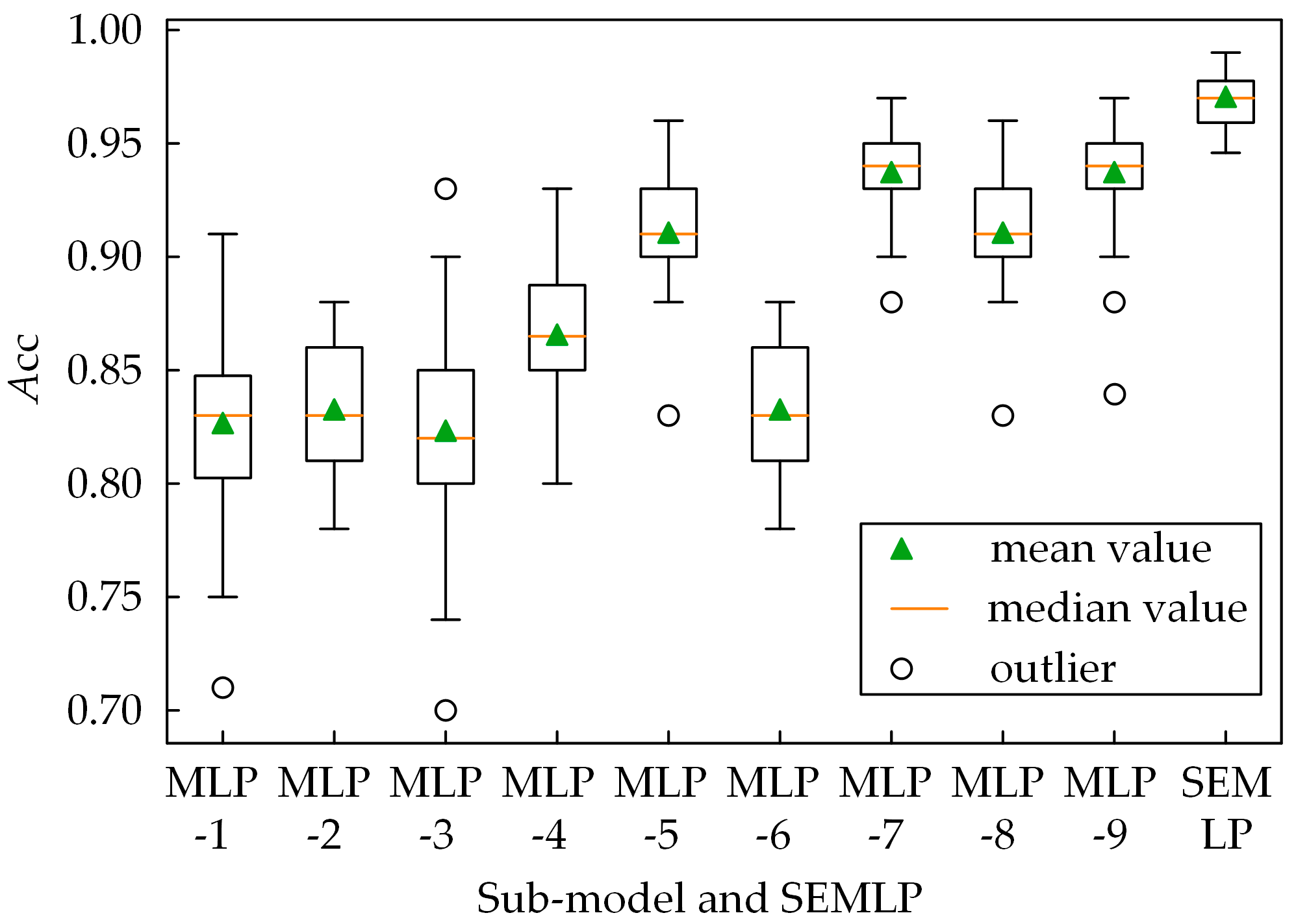
To ascertain the efficacy of the proposed SEMLP model, a comparison analysis was carried out to evaluate the accuracy of TSA among both the individual base classifiers and SEMLP within the framework of this research. The 10-fold cross-validation technique was utilized and repeated three times to demonstrate the average performance of the algorithms. The results of each sub-model and the SEMLP model were systematically summarized and displayed in box plots, as shown in Figure 7.
Observably, the SEMLP model stands out among the other individual sub-models with optimal performance, as reflected by its higher mean and median values. Such results effectively illustrate the superiority of the integrated model over the individual MLP models, thus attesting to the efficacy of the proposed SEMLP model in enhancing the accuracy of the underlying model.
4.3. Sensitivity Analysis
According to Section 2.5, the sensitivity of the active power of each generator with respect to TSI can be calculated. The result is shown in Figure 8. Positive sensitivities are indicated with red colors, while negative sensitivities are depicted in blue. The closeness of the colors to the color scale’s limits denotes the degree of sensitivity of the generator to TSI.
The sensitivity of each generator towards TSI exhibits a considerable disparity. Generators with high sensitivity are suitable for regulation during generation rescheduling. When , increasing the output power of the generator can reduce the degree of instability. Reversely, means that decreasing the output power of the generator can reduce the degree of instability. The projection of the surface onto the XY-plane can be observed in Figure 8. It is obvious that generators 5, 6, and 7 possess the highest sensitivity (absolute value) among all 10 generators, as indicated by their blue projections, thereby placing them within the negatively adjusted generator sequence. According to (9)~(14), the positive and negative adjustment sorts can be formed and incorporated into the initial sample set as prior knowledge for subsequent optimization algorithms.
4.4. Analysis of SEMLP-Driven AFO TSPC Method’s Results
The contingency set of the test system in this research is shown in Table 4.
As shown in Table 4, the system is found to be unstable at the selected insecure initial operating point when encountering a 3-phase-ground fault on Fault Lines 3–4 or Fault Lines 28–29.
In order to mitigate the adverse effects of contingencies and adjust the system to a secure operating point, the SEMLP-based TSA is integrated into the AFO algorithm for transient stability preventive control. A comparison of generators’ output before and after TSPC is shown in Figure 9.
To further demonstrate the economic performance of the TSPC method proposed in this research, Table 5 illustrates the control cost of TSPC.
Table 5 presents the total control cost amounting to USD 142.25. Notably, PG6 records the maximum decrease in power output. Intriguingly, this does not translate to a high control cost, a trend that is also evident for PG5, PG7, and PG9. This occurrence can be attributed to the optimization algorithm’s efforts in minimizing the scheduling cost during the generation scheduling process. This outcome demonstrates the economy of the proposed TSPC method.
To further verify the effectiveness of the proposed TSPC method, PSASP7.50 software is used to compare rotor angle trajectories before and after TSPC for unstable samples, specifically for Fault Lines 3–4 and Fault Lines 28–29. Figure 10 and Figure 11 demonstrate the results of this analysis.
The outcomes from the comparison indicate a significant improvement in stability after implementing the TSPC method. Specifically, all previously divergent rotor angle trajectories have now stabilized. This result serves as a compelling validation of the effectiveness of the proposed model.
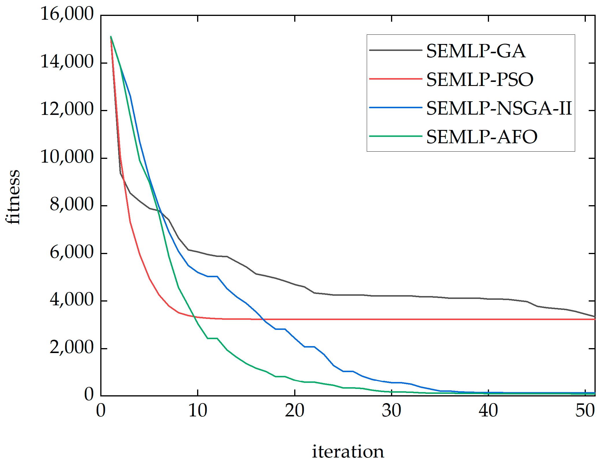
To showcase the superior convergence qualities of the SEMLP-AFO algorithm, this research conducts experiments comparing SEMLP with several widely adopted optimization algorithms. The detailed results of these experiments can be found in Figure 12.
As Figure 12 shows, the fitness values of the traditional population intelligence methods PSO and GA eventually converge to about 3000, while the final fitness values of the AFO algorithm and NSGA-II algorithm are close to the zero value. Furthermore, it is noteworthy that the AFO algorithm demonstrates faster convergence when compared to the NSGA-II algorithm. These results show the superior performance of the naturally inspired optimization algorithm in terms of convergence.
This research introduces the SEMLP-driven AFO preventive control algorithm, which addresses the need for rapidity in addition to ensuring effectiveness, stability, and economy.
Figure 13 provides clear evidence of the significant advantages of the proposed method in terms of rapidity. NSGA-II with time-domain simulation takes up to 3320 s due to the need to solve nonlinear differential-algebraic equations. In other studies, NSGA-II with a DBN-based TSA method takes 55 s. Additionally, a time reduction of 12 s is achieved by replacing the TSA model with the SEMLP method proposed in this paper. Finally, in this paper, AFO with SEMLP-based TSA algorithm only requires 35 s, demonstrating superior performance. Additional improvements in rapidity can be achieved by including sensitivity analysis.
4.5. TSPC Experiment Based on IEEE 300-Bus System
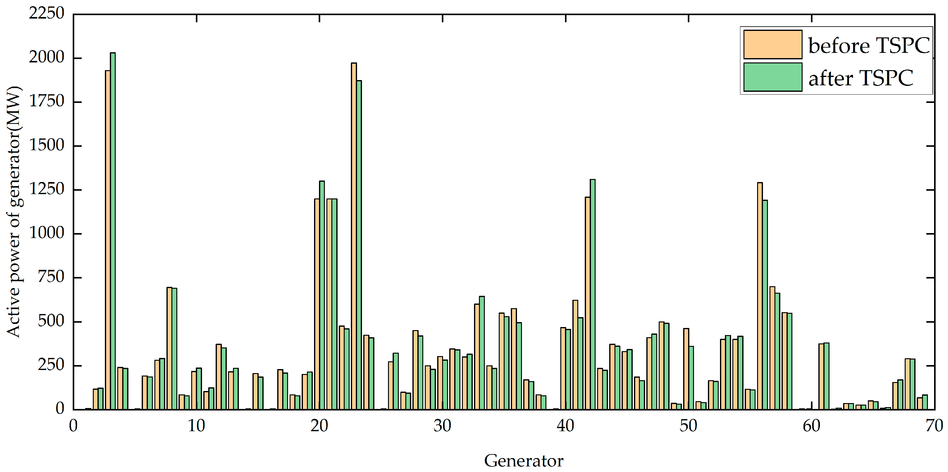
The IEEE 69-machine 300-bus system, which represents a larger regional interconnected grid, is employed for TSA in this research. PSASP software is utilized to generate sample data through simulation experiments. The active power of the loads and generator outputs is intentionally varied between 90% and 110%. A stochastic sampling technique is employed to choose 5000 operating points from the available pool of power system operating points. Two three-phase short circuit faults are selected to participate in the sample generation process, called Fault 1 and Fault 2. The simulation lasts 5 s, with the fault happening at t = 1 s and being resolved at t = 1.10 s. A comparison of generators’ output before and after TSPC is shown in Figure 14.
To verify the effectiveness of the proposed TSPC method in the IEEE 300-bus system, PSASP software is used to compare rotor angle trajectories before and after TSPC for unstable samples, namely Fault 1 and Fault 2. Figure 15 and Figure 16 demonstrate the results of the comparison.
After conducting preventive control using the proposed model, it is evident that all previously diverging rotor angle trajectories have been stabilized, thus demonstrating the effectiveness of the model. The convergence of rotor angle trajectories after TSPC is superior in the large system as compared to the IEEE 39-bus system, owing to the robust grid structure of the former. The experiments based on the IEEE 39-bus system and IEEE 300-bus system indicate that the proposed method can address stability concerns in real-time applications in both small- and large-scale power systems.
5. Conclusions
In this paper, a novel TSPC method driven by naturally inspired optimization with an improved transient stability assessment model is proposed. This method provides a smooth reconciliation of stability, economy, and rapidity when generation rescheduling.
- Stability. The stacking ensemble multilayer perceptron (SEMLP) approach is introduced to determine the transient stability of the system. The two-layer integrated model is designed in this paper to extract valuable information from diverse system operational features, thereby enhancing the overall model’s generalizability and accuracy. Based on this method, an online TSA model is developed and serves to determine the transient stability for TSPC. Experimental validation has demonstrated that the TSA model proposed in this paper possesses a significant advantage in terms of accuracy.
- Economy. The TSPC method, AFO driven by SEMLP, is developed to minimize generator adjustment costs. This method offers control strategies that are highly effective in achieving near-optimal operational costs while ensuring optimal system performance and operational economy.
- Rapidity. The rapidity of the TSPC method can be attributed to the sensitivity analysis and the excellent performance of the SEMLP-AFO model. The sensitivity analysis provides prior knowledge that aids in identifying and addressing issues promptly, while the SEMLP-AFO model’s robust performance ensures that the method performs effectively and efficiently.
There is still opportunity for refinement and enhancement of the methods implemented in this work. Future work is summarized as follows:
- In future work, the proposed method will be tested using practical systems and data.
- An integrated assessment model for power system transient stability can be developed. Power system transient stability can be classified into three categories: rotor angle stability, frequency stability, and voltage stability. This paper focuses on rotor angle transient stability. Future research is going to develop data-driven TSA methods to perform more precise, quick, reliable, and useful stability assessments in voltage stability and frequency stability.
Author Contributions
Conceptualization, Z.X. and D.Z.; methodology, Z.X. and W.H.; software, Z.X.; validation, Z.X., D.Z. and W.H.; formal analysis, Z.X.; investigation, Z.X. and X.H.; resources, Z.X., X.H. and W.H.; data curation, Z.X.; writing—original draft preparation, Z.X.; writing—review and editing, D.Z.; visualization, Z.X.; supervision, D.Z.; project administration, X.H.; funding acquisition, W.H. All authors have read and agreed to the published version of the manuscript.
Funding
This research was funded by the Science and Technology Project of the Central China Branch of State Grid Corporation of China, grant number 5214DK210014.
Data Availability Statement
Data are contained within the article.
Conflicts of Interest
Author Dongxia Zhang was employed by the company China Electric Power Research Institute. The authors declare that this study received funding from Central China Branch of State Grid Corporation of China. The remaining authors declare that the research was conducted in the absence of any commercial or financial relationships that could be construed as a potential conflict of interest.
References
- Xu, Y.; Zhang, W.; Chow, M.-Y.; Sun, H.; Gooi, H.B.; Peng, J. A Distributed Model-Free Controller for Enhancing Power System Transient Frequency Stability. IEEE Trans. Ind. Inform. 2019, 15, 1361–1371. [Google Scholar] [CrossRef]
- Yousefian, R.; Bhattarai, R.; Kamalasadan, S. Transient Stability Enhancement of Power Grid with Integrated Wide Area Control of Wind Farms and Synchronous Generators. IEEE Trans. Power Syst. 2017, 32, 4818–4831. [Google Scholar] [CrossRef]
- Hakami, A.; Hasan, K.; Alzubaidi, M.; Datta, M. A Review of Uncertainty Modelling Techniques for Probabilistic Stability Analysis of Renewable-Rich Power Systems. Energies 2023, 16, 112. [Google Scholar] [CrossRef]
- Kundur, P. Power System Stability and Control; McGraw Hill Education: New York, NY, USA, 2002. [Google Scholar]
- Chiang, H.-D. Direct Methods for Stability Analysis of Electric Power Systems: Theoretical Foundation, BCU Methodologies, and Applications; John Wiley & Sons: Hoboken, NJ, USA, 2010. [Google Scholar]
- Zhang, S.; Zhu, Z.; Li, Y. A Critical Review of Data-Driven Transient Stability Assessment of Power Systems: Principles, Prospects and Challenges. Energies 2021, 14, 7238. [Google Scholar] [CrossRef]
- Lee, H.; Kim, J.; Park, J.H.; Chung, S.-H. Power System Transient Stability Assessment Using Convolutional Neural Network and Saliency Map. Energies 2023, 16, 7743. [Google Scholar] [CrossRef]
- Wehenkel, L.; Van Cutsem, T.; Ribbens-Pavella, M. An Artificial Intelligence Framework for On-Line Transient Stability Assessment of Power Systems. IEEE Power Eng. Rev. 1989, 9, 77–78. [Google Scholar] [CrossRef]
- Hossain, E.; Khan, I.; Un-Noor, F.; Sikander, S.S.; Sunny, M.S.H. Application of Big Data and Machine Learning in Smart Grid, and Associated Security Concerns: A Review. IEEE Access 2019, 7, 13960–13988. [Google Scholar] [CrossRef]
- Hamilton, R.; Papadopoulos, P.; Bukhsh, W.; Bell, K. Identification of Important Locational, Physical and Economic Dimensions in Power System Transient Stability Margin Estimation. IEEE Trans. Sustain. Energy 2022, 13, 1135–1146. [Google Scholar] [CrossRef]
- Wang, H.; Hu, L.; Zhang, Y. SVM Based Imbalanced Correction Method for Power Systems Transient Stability Evaluation. ISA Trans. 2022, 136, 245–253. [Google Scholar] [CrossRef]
- Zhang, N.; Qian, H.; He, Y.; Li, L.; Sun, C. A Data-Driven Method for Power System Transient Instability Mode Identification Based on Knowledge Discovery and XGBoost Algorithm. IEEE Access 2021, 9, 154172–154182. [Google Scholar] [CrossRef]
- Goodfellow, I.; Bengio, Y.; Courville, A. Deep Learning; MIT Press: Cambridge, MA, USA, 2016. [Google Scholar]
- Zhang, Y.; Shi, X.; Zhang, H.; Cao, Y.; Terzija, V. Review on Deep Learning Applications in Frequency Analysis and Control of Modern Power System. Int. J. Electr. Power Energy Syst. 2022, 136, 107744. [Google Scholar] [CrossRef]
- Wu, S.; Zheng, L.; Hu, W.; Yu, R.; Liu, B. Improved Deep Belief Network and Model Interpretation Method for Power System Transient Stability Assessment. J. Mod. Power Syst. Clean Energy 2020, 8, 27–37. [Google Scholar] [CrossRef]
- Zhou, Y.; Guo, Q.; Sun, H.; Yu, Z.; Wu, J.; Hao, L. A Novel Data-Driven Approach for Transient Stability Prediction of Power Systems Considering the Operational Variability. Int. J. Electr. Power Energy Syst. 2019, 107, 379–394. [Google Scholar] [CrossRef]
- Ren, C.; Xu, Y. A Fully Data-Driven Method Based on Generative Adversarial Networks for Power System Dynamic Security Assessment With Missing Data. IEEE Trans. Power Syst. 2019, 34, 5044–5052. [Google Scholar] [CrossRef]
- Ruiz-Vega, D.; Pavella, M. A Comprehensive Approach to Transient Stability Control Part 1: Near Optimal Preventive Control. In Proceedings of the 2003 IEEE Power Engineering Society General Meeting (IEEE Cat. No.03CH37491), Toronto, ON, Canada, 13–17 July 2003; Volume 3, p. 1810. [Google Scholar]
- Hatziargyriou, N.; Milanovic, J.; Rahmann, C.; Ajjarapu, V.; Canizares, C.; Erlich, I.; Hill, D.; Hiskens, I.; Kamwa, I.; Pal, B.; et al. Definition and Classification of Power System Stability—Revisited & Extended. IEEE Trans. Power Syst. 2021, 36, 3271–3281. [Google Scholar] [CrossRef]
- Gan, D.; Thomas, R.; Zimmerman, R. Stability-Constrained Optimal Power Flow. IEEE Trans. Power Syst. 2000, 15, 535–540. [Google Scholar] [CrossRef]
- Yuan, Y.; Kubokawa, J.; Sasaki, H. A Solution of Optimal Power Flow with Multicontingency Transient Stability Constraints. IEEE Trans. Power Syst. 2003, 18, 1094–1102. [Google Scholar] [CrossRef]
- Yang, Y.; Liu, Y.; Liu, J.; Huang, Z.; Liu, T.; Qiu, G. Preventive Transient Stability Control Based on Neural Network Security Predictor. Power Syst. Technol. 2018, 42, 4076–4084. [Google Scholar]
- Su, T.; Liu, Y.; Zhao, J.; Liu, J. Deep Belief Network Enabled Surrogate Modeling for Fast Preventive Control of Power System Transient Stability. IEEE Trans. Ind. Inform. 2022, 18, 315–326. [Google Scholar] [CrossRef]
- Dong, X.; Yu, Z.; Cao, W.; Shi, Y.; Ma, Q. A Survey on Ensemble Learning. Front. Comput. Sci. 2020, 14, 241–258. [Google Scholar] [CrossRef]
- Shi, J.; Zhang, J. Load Forecasting Based on Multi-Model by Stacking Ensemble Learning. Proc. Chin. Soc. Electr. Eng. 2019, 39, 4032–4041. [Google Scholar]
- Yang, Z.; Deng, L.; Wang, Y.; Liu, J. Aptenodytes Forsteri Optimization: Algorithm and Applications. Knowl. Based Syst. 2021, 232, 107483. [Google Scholar] [CrossRef]
Figure 1.
Network structure of MLP.

Figure 2.
Structural diagram of stacking ensemble learning.

Figure 3.
Model structure of TSA based on SEMLP.

Figure 4.
Model structure of SEMLP-AFO.

Figure 5.
Proposed AFO driven by SEMLP model for TSPC.

Figure 6.
SEMLP-based TSA’s performance: (a) accuracy; (b) loss.

Figure 7.
The performance comparison between SEMLP-based TSA and each sub-classifier. (Box plots show the middle 50% of each data distribution).
Figure 7.
The performance comparison between SEMLP-based TSA and each sub-classifier. (Box plots show the middle 50% of each data distribution).

Figure 8.
The sensitivity of generator output with respect to TSI.

Figure 9.
Comparison of generators’ output before and after TSPC in IEEE 39 bus system.

Figure 10.
Fault bus-3_bus-4’s rotor angle trajectories (a) before TSPC; (b) after TSPC.

Figure 11.
Fault bus-28_bus-29’s rotor angle trajectories (a) before TSPC; (b) after TSPC.

Figure 12.
Convergence curve of different optimization algorithms with SEMLP as TSA.

Figure 13.
Comparison of time consumption of different TSPC methods.

Figure 14.
Comparison of generators’ output before and after TSPC in IEEE 300 bus system..

Figure 15.
Fault 1’s rotor angle trajectories (a) before TSPC; (b) after TSPC.

Figure 16.
Fault 2’s rotor angle trajectories (a) before TSPC; (b) after TSPC.


Table 1.
SEMLP model structure parameters.
| Sub-Model | Hidden Layer | Neuronal Count per Layer (from Left to Right) |
|---|---|---|
| MLP-1 | 3 | (64, 32, 16) |
| MLP-2 | 4 | (128, 64, 32, 16) |
| MLP-3 | 5 | (256, 128, 64, 32, 16) |
| MLP-4 | 3 | (64, 32, 16) |
| MLP-5 | 4 | (128, 64, 32, 16) |
| MLP-6 | 5 | (256, 128, 64, 32, 16) |
| MLP-7 | 3 | (64, 32, 16) |
| MLP-8 | 4 | (128, 64, 32, 16) |
| MLP-9 | 5 | (256, 128, 64, 32, 16) |
| Meta-classifier MLP | 3 | (64, 32, 16) |
Table 2.
Results of TSA.
| Real Label | Predicted Results of TSA | |
|---|---|---|
| Stable (Predicted) | Unstable (Predicted) | |
| Stable (actual) | TP | FN |
| Unstable (actual) | FP | TN |
Table 3.
Performance of different TSA models.
| RF | SVM | CNN | SAE | DBN | SEMLP | |
|---|---|---|---|---|---|---|
| Acc/% | 89.92 | 93.55 | 94.56 | 95.95 | 96.24 | 98.55 |
| TPR/% | 90.42 | 94.94 | 95.80 | 97.33 | 97.61 | 98.64 |
| TNR/% | 87.02 | 91.45 | 92.68 | 94.00 | 94.83 | 98.45 |
| Gmean/% | 88.70 | 93.18 | 94.23 | 95.65 | 96.21 | 98.54 |
Table 4.
Contingency set of IEEE 39-bus system.
| Contingency No. | Fault Line | Fault Bus | Stable State |
|---|---|---|---|
| 1 | 2–3 | 2 or 3 | Stable |
| 2 | 3–4 | 3 or 4 | Unstable |
| 3 | 4–5 | 4 or 5 | Stable |
| 4 | 4–14 | 4 or 14 | Stable |
| 5 | 5–6 | 5 or 6 | Stable |
| 6 | 5–8 | 5 or 8 | Stable |
| 7 | 10–13 | 10 or 13 | Stable |
| 8 | 19–20 | 19 or 20 | Stable |
| 9 | 23–24 | 23 or 24 | Stable |
| 10 | 28–29 | 28 or 29 | Unstable |
Table 5.
Cost of TSPC.
| Generator | Before TSPC/MW | After TSPC/MW | Output Change/MW | Unit Adjustment Cost | Gen. Cost |
|---|---|---|---|---|---|
| 1 | 249.57 | 254.72 | 5.15 | 1 | 142.425 |
| 2 | 687.28 | 685.74 | −1.54 | 1 | |
| 3 | 648.89 | 672.35 | 23.46 | 1 | |
| 4 | 630.92 | 626.74 | −4.18 | 0.5 | |
| 5 | 507.13 | 478.73 | −28.40 | 0.5 | |
| 6 | 648.89 | 601.41 | −47.48 | 0.5 | |
| 7 | 559.04 | 531.04 | −28 | 0.5 | |
| 8 | 539.08 | 575.03 | 35.95 | 1 | |
| 9 | 828.58 | 872.72 | 44.14 | 0.5 | |
| 10 | 998.29 | 998.74 | 0.45 | 0.5 |
Disclaimer/Publisher’s Note: The statements, opinions and data contained in all publications are solely those of the individual author(s) and contributor(s) and not of MDPI and/or the editor(s). MDPI and/or the editor(s) disclaim responsibility for any injury to people or property resulting from any ideas, methods, instructions or products referred to in the content. |
© 2024 by the authors. Licensee MDPI, Basel, Switzerland. This article is an open access article distributed under the terms and conditions of the Creative Commons Attribution (CC BY) license (https://creativecommons.org/licenses/by/4.0/).
Share and Cite
MDPI and ACS Style
Xie, Z.; Zhang, D.; Hu, W.; Han, X. Power System Transient Stability Preventive Control via Aptenodytes Forsteri Optimization with an Improved Transient Stability Assessment Model. Energies 2024, 17, 1942. https://doi.org/10.3390/en17081942
AMA Style
Xie Z, Zhang D, Hu W, Han X. Power System Transient Stability Preventive Control via Aptenodytes Forsteri Optimization with an Improved Transient Stability Assessment Model. Energies. 2024; 17(8):1942. https://doi.org/10.3390/en17081942
Chicago/Turabian StyleXie, Zhijun, Dongxia Zhang, Wei Hu, and Xiaoqing Han. 2024. "Power System Transient Stability Preventive Control via Aptenodytes Forsteri Optimization with an Improved Transient Stability Assessment Model" Energies 17, no. 8: 1942. https://doi.org/10.3390/en17081942
Note that from the first issue of 2016, this journal uses article numbers instead of page numbers. See further details here.