Collaborative Optimization Scheduling of Multi-Microgrids Incorporating Hydrogen-Doped Natural Gas and P2G–CCS Coupling under Carbon Trading and Carbon Emission Constraints

Abstract

In the context of “dual carbon”, restrictions on carbon emissions have attracted widespread attention from researchers. In order to solve the issue of the insufficient exploration of the synergistic emission reduction effects of various low-carbon policies and technologies applied to multiple microgrids, we propose a multi-microgrid electricity cooperation optimization scheduling strategy based on stepped carbon trading, a hydrogen-doped natural gas system and P2G–CCS coupled operation. Firstly, a multi-energy microgrid model is developed, coupled with hydrogen-doped natural gas system and P2G–CCS, and then carbon trading and a carbon emission restriction mechanism are introduced. Based on this, a model for multi-microgrid electricity cooperation is established. Secondly, design optimization strategies for solving the model are divided into the day-ahead stage and the intraday stage. In the day-ahead stage, an improved alternating direction multiplier method is used to distribute the model to minimize the cooperative costs of multiple microgrids. In the intraday stage, based on the day-ahead scheduling results, an intraday scheduling model is established and a rolling optimization strategy to adjust the output of microgrid equipment and energy purchases is adopted, which reduces the impact of uncertainties in new energy output and load forecasting and improves the economic and low-carbon operation of multiple microgrids. Setting up different scenarios for experimental validation demonstrates the effectiveness of the introduced low-carbon policies and technologies as well as the effectiveness of their synergistic interaction.

1. Introduction

Dual carbon goals have prompted existing research to focus on the low-carbon optimization of multi-microgrids. There are several ways to achieve this: either through the implementation of low-carbon policies, such as carbon trading or carbon trading markets [1,2,3,4,5], or by employing low-carbon technologies, such as the individual or combined use of carbon capture technology, electrolytic hydrogen production technology, and other low-carbon technologies [6,7,8,9,10]. These measures have effectively reduced the carbon emissions of multi-microgrids and have enhanced their environmental friendliness.

Regarding low-carbon policies, Reference [11] established a model focusing on carbon emissions. Based on the carbon trading mechanism, a cooperative model was proposed to determine optimal power trading [12], and Reference [13] established a low-carbon transaction mechanism based on the carbon trading mechanism and the Stackelberg game theory, and Reference [14] developed a trading strategy between multiple entities in the system using the double Stackelberg game framework, focusing on the uncertainty of the carbon trading mechanism. Reference [15] established an integrated energy microgrid (IEM) model focusing on carbon trading. On this basis, a multi-IEM collaborative operation model was constructed. Reference [16] established a multi-microgrid system with a comprehensive and flexible operation mode based on the carbon trading mechanism, and the carbon trading mechanism was also introduced by Reference [17] to establish a low-carbon optimization scheduling model of multi-microgrids. In Reference [18], carbon emission and green certificate trading were introduced to establish a multi-microgrid cooperative transaction model, focusing on the coupling of energy and carbon. A double-layer electric heating and sharing model of multi-microgrids was constructed, and the carbon trading mechanism was introduced by Reference [19]. Reference [20] proposed a local power- and carbon-trading method for interconnecting multi-energy microgrids, introducing a carbon trading mechanism, and Reference [21] established a multi-microgrids collaborative operation model, in which the ladder carbon trading mechanism was considered.

Regarding low-carbon technology, Reference [22] established a coupling operation framework for a combined heat and power generation and a power-togas and carbon capture system, and integrated this with a carbon trading mechanism to reduce carbon emissions. Reference [23] established a multi-agent cooperative operation model based on Nash bargaining theory, adding carbon capture systems and power-to-gas devices to the sub-model under the constraints of comprehensive demand response and carbon trading. Reference [24] constructed a microgrid model integrating electricity-to-gas and carbon capture systems, and a multi-energy coordinated microgrid model and an optimal scheduling scheme for a regional integrated energy system cluster (RIESG), which combined power-to-gas and inter-park power assistance, was proposed by Reference [25]. In Reference [26], a cooperative model of multi-microgrids was established, and a power-to-hydrogen device was added to the model.

In conclusion, current research has demonstrated that low-carbon policies, represented by carbon trading and low-carbon technologies as well as carbon capture systems, have effectively reduced emissions in industry. It is evident that the combined applications of various emission reduction policies and technologies will become a research focus in the future for the power system research field. Therefore, the synergistic application of multiple low-carbon policies and technologies, within the cooperative optimization scheduling of multi-microgrids, holds significant research significance. It provides a feasible approach for exploring the low-carbon operation of the power system.

This paper proposes a multi-microgrids electric energy cooperation optimization scheduling strategy based on carbon trading and carbon emission constraints, including P2G–CCS coupling and hydrogen-doped natural gas system. Firstly, it establishes a multi-energy microgrid model incorporating hydrogen-doped natural gas and a P2G–CCS coupling system, and it introduces a tiered carbon trading and carbon emission constraint mechanism. Based on this, a model for multi-microgrid electric energy cooperation is established. Secondly, the optimization strategy for solving the model is designed with the two following stages: the day-ahead and intraday stages. In the day-ahead stage, an alternating direction multiplier method is used for the distributed solving of the model, thereby minimizing the cooperative cost of multi-microgrids; in the intraday stage, an intraday scheduling model is established, based on the day-ahead scheduling results. A rolling optimization strategy is adopted to adjust the output of the microgrid devices and the amount of energy purchases, reducing the impact of uncertainty in the renewable energy and load forecasting and improving the economic and low-carbon operation of multiple microgrids. Finally, different scenarios are set, to demonstrate the proposed method’s in-depth analysis of the cost and carbon emissions impact on multiple microgrids under the coordination of low-carbon policies and technologies.

2. Multi-Microgrids Model

Figure 1 is the model of the multi-microgrids.

As shown in Figure 1, a multi-microgrid (MMG) is a highly intelligent and flexible energy system composed of multiple microgrids. Each microgrid functions as a small-scale energy system, and energy sharing among different subsystems within the multi-microgrids is achieved through the flow of electrical energy. This enables the efficient utilization and flexible distribution of energy within the system. In addition to energy sharing among subsystems, connections to the main power grid and gas networks provide backup energy sources and flexibility for the multi-microgrid system.

In order to analyze the microgrid energy flow, Figure 2 shows the multi-energy microgrid model incorporating P2G–CCS coupling and a hydrogen-doped natural gas system.

As shown in Figure 2, the model includes renewable energy generation, a combined heat and power (CHP) unit, a gas boiler (GB), a two-stage power-to-gas (P2G) system (the system includes a power-to-hydrogen (P2H) and a methanation unit), a heat pump (HP), and a carbon capture system (CCS; this system includes carbon storage and liquid storage), as well as electric energy storage (ES), heat storage (HS), and a hydrogen storage system (HSS).

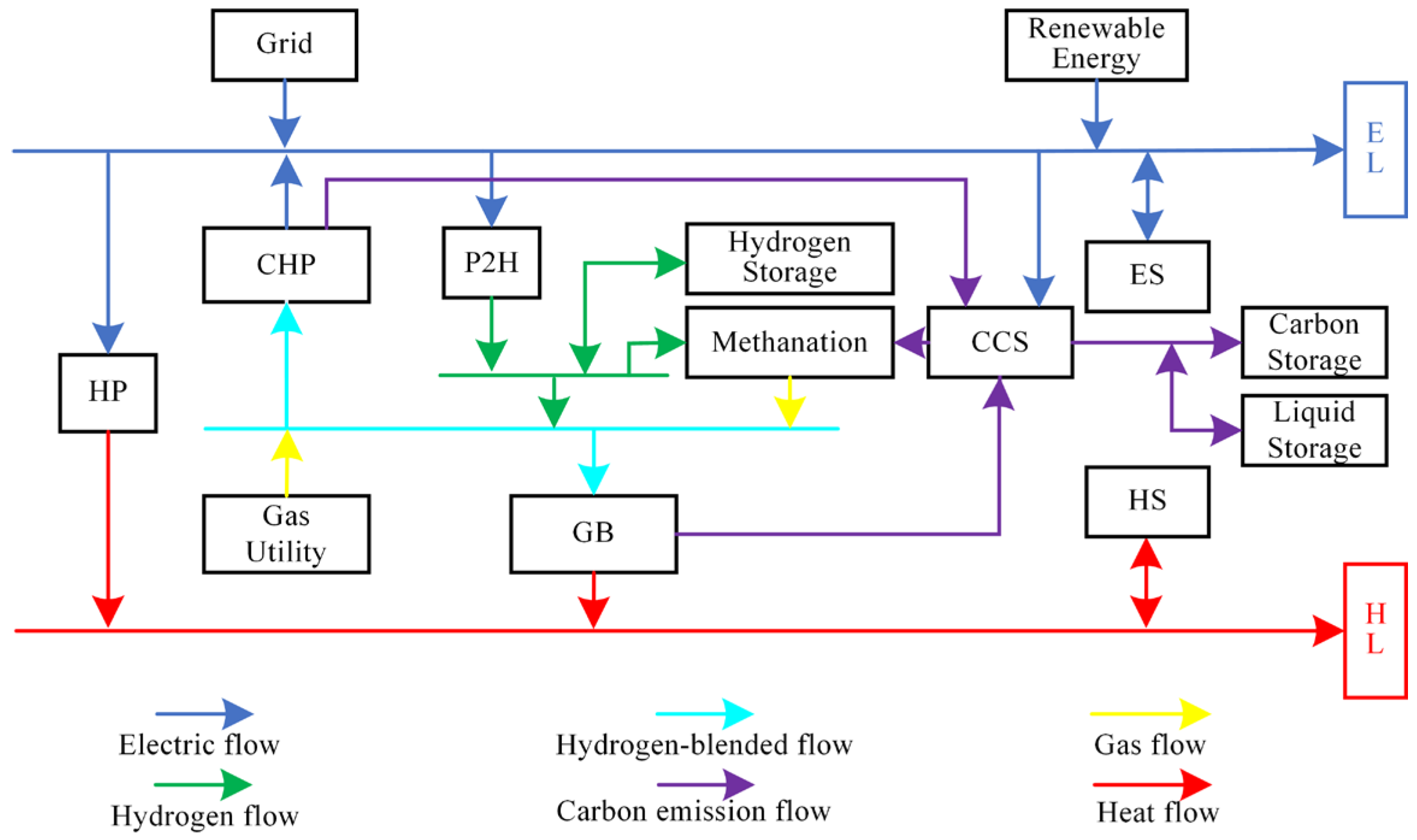
3. Modeling of Hydrogen-Doped Natural Gas and P2G–CCS Coupling

Figure 3 is the subsystem structure of P2G–CCS coupling and hydrogen-doped natural gas.

In Figure 3, the multi-microgrid system generates a certain amount of carbon dioxide during its operation. There are various pathways and methods for handling these carbon emissions. Some of them are directly emitted into the atmosphere through flue gas diversion, while another portion is sent to the CCS facilities for treatment. However, as carbon capture technology is not 100% efficient, a portion of the carbon dioxide treated by the CCS facility is indirectly emitted into the atmosphere. Within the carbon capture and storage facility, a portion of the carbon dioxide is used as feedstock for methanation and sent to the P2G facility. In this process, carbon dioxide reacts with hydrogen to form methane, thus enabling the coupled operation of P2G and CCS. This coupled operation not only helps reduce the carbon dioxide content in the atmosphere but also generates renewable natural gas resources, enabling carbon recycling. Another portion of the carbon dioxide treated by the carbon capture and carbon storage facility undergoes carbon sequestration. The P2G process is refined into two stages: P2H and methane production. Firstly, there is the electrolysis process for hydrogen production. In this stage, electrical energy is consumed to generate hydrogen gas. A portion of the hydrogen is supplied to the CHP and the GB units, while the remaining part undergoes methane production. In the methane production process, methane is produced by the reaction of hydrogen with captured carbon dioxide, which is then injected into the natural gas supply.

3.1. Modeling of P2G–CCS Coupling

(1)

Carbon Capture System model

In order to exploit the low-carbon potential, a CCS facility with a liquid storage unit is employed. $P_{i,t}^{\mathrm{ccssum}}$ consists of fixed energy consumption $P_{i,t}^{\mathrm{b}}$ and operational energy consumption $P_{i,t}^{\mathrm{ccs}}$, and the expression is as follows:

$$P_{i,t}^{\mathrm{ccs}}=e_{\mathrm{c}}{E}_{i,t}^{\mathrm{ccs}}$$

(1)

$$P_{i,t}^{\mathrm{ccssum}}=P_{i,t}^{\mathrm{b}}+P_{i,t}^{\mathrm{ccs}}$$

(2)

$$0\le P_{i,t}^{\mathrm{ccs}}\le P_{i,\max }^{\mathrm{ccs}}$$

(3)

$$P_{i,\min }^{\mathrm{ccssum}}\le P_{i,t}^{\mathrm{ccssum}}\le P_{i,\max }^{\mathrm{ccssum}}$$

(4)

In Equations (1)–(4), Equation (1) calculates the energy conversion between the operating power consumed by the CCS and the mass of CO₂ treated, Equation (2) calculates the total power consumption of the CCS, and Equations (3) and (4) calculate the CCS operating power and total power constraints, respectively. $e_{\mathrm{c}}$ represents the unit energy consumption coefficient for processing carbon dioxide, which is 0.269; $E_{i,t}^{\mathrm{ccs}}$ denotes the amount of CO₂ absorbed by the CCS unit in microgrid i at time t; $P_{i,\max }^{\mathrm{ccs}}$ denotes the maximum operating power of the CCS unit in microgrid i; and $P_{i,t}^{\mathrm{ccssum}}$ is the total power of CCS unit in microgrid i at time t, and it ranges from its minimum value, $P_{i,\min }^{\mathrm{ccssum}}$, to its maximum value, $P_{i,\max }^{\mathrm{ccssum}}$.

The CCS unit employed in this paper introduces a flue gas bypass system and a liquid storage unit. The specific expressions are as follows:

$$\left\{\begin{array}{l}{E}_{i,t}^{\mathrm{ccs}}=E_{i,t}^{\mathrm{sum}}-E_{i,t}^{\mathrm{air}}\\ E_{i,t}^{\mathrm{ccs}}=\frac{1}{{\eta }_i^{\mathrm{C}}}(E_{i,t}^{\mathrm{H}2\mathrm{G}}+E_{i,t}^{\mathrm{STO}}+E_{i,t}^{\mathrm{ca}})\end{array}\right.$$

(5)

Equation (5) calculates the mass of CO₂ treated by the CCS. In Equation (5), $E_{i,t}^{\mathrm{sum}}$ is the total amount of carbon emissions from the units in microgrid i at time t, $E_{i,t}^{\mathrm{air}}$ is the amount of CO₂ emitted into the atmosphere by the units in microgrid i at time t, $E_{i,t}^{\mathrm{ca}}$ is the amount of CO₂ provided by the liquid storage unit in microgrid i at time t, $E_{i,t}^{\mathrm{H}2\mathrm{G}}$ represents the amount of CO₂ utilized for methanation from the CCS in microgrid i at time t, $E_{i,t}^{\mathrm{STO}}$ represents the amount of CO₂ stored from the CCS in microgrid i at time t, and ${\eta }_i^{\mathrm{C}}$ represents the efficiency of the CCS unit in microgrid i.

The constraint for the emissions into the atmosphere from the CCS unit is as follows:

$$\left\{\begin{array}{l}0\le E_{i,t}^{\mathrm{air}}\le E_{i,\max }^{\mathrm{air}}\\ E_{i,\max }^{\mathrm{air}}={\sigma }_{\mathrm{c}}{E}_{i,t}^{\mathrm{sum}}\end{array}\right.$$

(6)

In Equation (6), $E_{i,\max }^{\mathrm{air}}$ is the maximum amount of carbon emissions released into the atmosphere by the units in microgrid i at time t, and ${\sigma }_{\mathrm{c}}$ denotes the gas partition coefficient for the CCS unit.

The liquid storage unit is an essential component of the CCS unit. Following the method proposed, carbon dioxide in the liquid storage unit exists in the form of compounds in amine solution. The expressions for the process are as follows [27]:

$$V_{i,t}^{\mathrm{ca}}=\frac{E_{i,t}^{\mathrm{ca}}{M}_{\mathrm{MEA}}{\theta }_i}{M_{{\mathrm{CO}}_2}{C}_{\mathrm{R}}{\rho }_{\mathrm{R}}}$$

(7)

$$E_{i,\min }^{\mathrm{ca}}\le E_{i,t}^{\mathrm{ca}}\le E_{i,\max }^{\mathrm{ca}}$$

(8)

In Equations (7) and (8), Equation (7) is the conversion equation for the liquid storage unit, Equation (8) is the constraint of the liquid storage unit, $V_{i,t}^{\mathrm{ca}}$ denotes the volume of CO₂ provided by the liquid storage unit installed in microgrid i at time t, $E_{i,\min }^{\mathrm{ca}}$ and $E_{i,\max }^{\mathrm{ca}}$ are the minimum and maximum volume of CO₂ provided by the liquid storage unit in microgrid i, $M_{\mathrm{MEA}}$ is the molar mass of monoethanolamine, ${\theta }_i$ is the conversion coefficient of the liquid storage unit in microgrid i, $C_{\mathrm{R}}$ is the concentration of monoethanolamine solution, ${\rho }_{\mathrm{R}}$ is the density of the monoethanolamine solution, and $M_{{\mathrm{CO}}_2}$ is the molar mass of CO₂.

The constraint expression for the liquid storage unit is given in Equation (9), as follows:

$$\left\{\begin{array}{l}{V}_{i,t}^{\mathrm{F}}=V_{i,t-1}^{\mathrm{F}}-V_{i,t}^{\mathrm{ca}}\hfill \\ V_{i,t}^{\mathrm{P}}=V_{i,t-1}^{\mathrm{P}}+V_{i,t}^{\mathrm{ca}}\hfill \\ 0\le V_{i,t}^{\mathrm{F}}\le V_i^{\mathrm{CR}}\hfill \\ 0\le V_{i,t}^{\mathrm{P}}\le V_i^{\mathrm{CR}}\hfill \\ V_{i,0}^{\mathrm{F}}=V_{i,24}^{\mathrm{F}}\hfill \\ V_{i,0}^{\mathrm{P}}=V_{i,24}^{\mathrm{P}}\hfill \end{array}\right.$$

(9)

In Equation (9), $V_{i,t}^{\mathrm{F}}=V_{i,t-1}^{\mathrm{F}}-V_{i,t}^{\mathrm{ca}}$ and $V_{i,t}^{\mathrm{P}}=V_{i,t-1}^{\mathrm{P}}+V_{i,t}^{\mathrm{ca}}$ are the expressions for the change in volume of the liquid-rich and liquid-poor units, respectively; $0\le V_{i,t}^{\mathrm{F}}\le V_i^{\mathrm{CR}}$ and $0\le V_{i,t}^{\mathrm{P}}\le V_i^{\mathrm{CR}}$ are the liquid-rich and liquid-poor unit constraints, respectively; and $V_{i,0}^{\mathrm{F}}=V_{i,24}^{\mathrm{F}}$ and $V_{i,0}^{\mathrm{P}}=V_{i,24}^{\mathrm{P}}$ are expressed as no change in the liquid-rich and liquid-poor unit reserves at the end of the dispatch cycle, respectively. $V_i^{\mathrm{CR}}$ is the capacity of the liquid storage unit in microgrid i; $V_{i,t}^{\mathrm{F}}$ and $V_{i,t}^{\mathrm{P}}$ are the reserves of the liquid storage units that store rich and lean liquid in microgrid i, respectively; $V_{i,0}^{\mathrm{F}}$ and $V_{i,0}^{\mathrm{P}}$ are the initial reserves of the liquid storage units storing liquid-rich and liquid-poor in microgrid i, respectively; and $V_{i,24}^{\mathrm{F}}$ and $V_{i,24}^{\mathrm{P}}$ are the final reserves of the liquid storage units storing liquid-rich and liquid-poor in microgrid i, respectively.

(2)

Two-stage Power-to-Gas model

This model, based on P2G, is subdivided into P2H and methanation steps. The model expression is as follows:

$$\left\{\begin{array}{l}{P}_{i,t}^{\mathrm{EL},{\mathrm{H}}_2}={\eta }_i^{\mathrm{EL}}{P}_{i,t}^{\mathrm{EL}}\hfill \\ P_{i,t}^{\mathrm{H}2\mathrm{G}, \mathrm{out} }={\eta }_i^{\mathrm{H}2\mathrm{G}}{P}_{i,t}^{\mathrm{H}2\mathrm{G}, \mathrm{in} }\hfill \end{array}\right.$$

(10)

In Equation (10), $P_{i,t}^{\mathrm{EL},{\mathrm{H}}_2}={\eta }_i^{\mathrm{EL}}{P}_{i,t}^{\mathrm{EL}}$ is the expression for P2H and $P_{i,t}^{\mathrm{H}2\mathrm{G}, \mathrm{out} }={\eta }_i^{\mathrm{H}2\mathrm{G}}{P}_{i,t}^{\mathrm{H}2\mathrm{G}, \mathrm{in} }$ is the expression for methanation. $P_{i,t}^{\mathrm{EL}}$ represents the electric power consumed by electrolysis in microgrid i at time t. $P_{i,t}^{\mathrm{EL},{\mathrm{H}}_2}$ represents the hydrogen production power consumed by electrolysis in microgrid i at time t. $P_{i,t}^{\mathrm{H}2\mathrm{G}, \mathrm{out} }$ denotes the methane production power of the methanation equipment in microgrid i at time t. $P_{i,t}^{\mathrm{H}2\mathrm{G}, \mathrm{in} }$ denotes the hydrogen consumption power of the methanation equipment in microgrid i at time t. ${\eta }_i^{\mathrm{EL}}$ and ${\eta }_i^{\mathrm{H}2\mathrm{G}}$ are the efficiencies of the P2H and methanation processes in microgrid i, respectively.

The constraints for the P2H process are as follows:

$$\left\{\begin{array}{l}{P}_{i,\min }^{\mathrm{EL}}\le P_{i,t}^{\mathrm{EL}}\le P_{i,\max }^{\mathrm{EL}}\hfill \\ P_{i,\mathrm{d}}^{\mathrm{EL}}\le P_{i,t}^{\mathrm{EL}}-P_{i,t-1}^{\mathrm{EL}}\le P_{i,\mathrm{up}}^{\mathrm{EL}}\hfill \end{array}\right.$$

(11)

In Equation (11), $P_{i,\min }^{\mathrm{EL}}\le P_{i,t}^{\mathrm{EL}}\le P_{i,\max }^{\mathrm{EL}}$ is the constraint on the P2H consumption of electrical energy, and $P_{i,\mathrm{d}}^{\mathrm{EL}}\le P_{i,t}^{\mathrm{EL}}-P_{i,t-1}^{\mathrm{EL}}\le P_{i,\mathrm{up}}^{\mathrm{EL}}$ is the constraint on the P2H consumption of the electrical energy climbing rate. $P_{i,\max }^{\mathrm{EL}}$ and $P_{i,\min }^{\mathrm{EL}}$ are the maximum and minimum electric power consumption for electrolysis in the P2H process in microgrid i at time t, respectively; $P_{i,\mathrm{up}}^{\mathrm{EL}}$ and $P_{i,\mathrm{d}}^{\mathrm{EL}}$ are the maximum and minimum climbing power in the P2H process in microgrid i at time t, respectively.

The expression for the consumption of carbon dioxide by the P2G unit can be represented as follows [28]:

$$E_{i,t}^{\mathrm{H}2\mathrm{G}}=\frac{3600P_{i,t}^{\mathrm{H}2\mathrm{G}, \mathrm{out} }{\rho }_{{\mathrm{CO}}_2}}{Q_{{\mathrm{CH}}_4}}$$

(12)

$$\left\{\begin{array}{l}{E}_{i,t}^{\mathrm{H}2\mathrm{G},\mathrm{SUM}}=E_{i,t}^{\mathrm{H}2\mathrm{G}}+E_{i,t}^{\mathrm{STO}}\\ E_{i,t}^{\mathrm{H}2\mathrm{G},\mathrm{SUM}}={\eta }_i^{\mathrm{C}}{E}_{i,t}^{\mathrm{ccs}}-E_{i,t}^{\mathrm{ca}}\end{array}\right.$$

(13)

The constraint for carbon storage is as follows:

$$0\le E_{i,t}^{\mathrm{STO}}\le E_{i,\max }^{\mathrm{STO}}$$

(14)

In Equations (12) and (13), Equation (12) is the conversion equation for CO₂ required for the methanation process and Equation (13) calculates the total mass of CO₂ consumed by the P2G unit. ${\rho }_{{\mathrm{CO}}_2}$ is the density of carbon dioxide, $E_{i,\max }^{\mathrm{STO}}$ is the maximum amount of carbon sequestration in microgrid i, and $E_{i,t}^{\mathrm{H}2\mathrm{G},\mathrm{SUM}}$ is the amount of CO₂ consumed by the P2G unit in microgrid i at time t.

As the volume of carbon dioxide consumed during the methanation process is consistent with the volume of methane generated, determining the required mass of carbon dioxide becomes a crucial step. This mass can be calculated using Equation (12). Equation (13) indicates that all the carbon dioxide required for methanation in the P2G unit comes from the CCS, thereby achieving the coupling of P2G–CCS and enhancing the economic and low-carbon operation of the unit.

3.2. Modeling of Hydrogen Blending in Combined Heat and Power Units and Gas Boilers

(1)

Hydrogen blending in combined heat and power units

When using CHP units with a certain proportion of hydrogen blended into natural gas, it is safe to burn natural gas with a hydrogen blending ratio of 10–20% [29]. The expression of the model is as follows:

$$\left\{\begin{array}{l}{P}_{i,t}^{\mathrm{e},\mathrm{chp}}={\eta }_i^{\mathrm{e},\mathrm{chp}}(P_{i,t}^{\mathrm{g},\mathrm{chp}}+P_{i,t}^{{\mathrm{h}}_2,\mathrm{chp}})\\ P_{i,t}^{\mathrm{h},\mathrm{chp}}={\eta }_i^{\mathrm{h},\mathrm{chp}}(P_{i,t}^{\mathrm{g},\mathrm{chp}}+P_{i,t}^{{\mathrm{h}}_2,\mathrm{chp}})\\ P_{i,t}^{\mathrm{g},\mathrm{chp}}=V_{i,t}^{\mathrm{g},\mathrm{chp}}{Q}_{{\mathrm{CH}}_4}\\ P_{i,t}^{{\mathrm{h}}_2,\mathrm{chp}}=V_{i,t}^{{\mathrm{h}}_2,\mathrm{chp}}{Q}_{{\mathrm{H}}_2}\\ Y_{i,t}^{{\mathrm{h}}_2,\mathrm{chp}}=V_{i,t}^{{\mathrm{h}}_2,\mathrm{chp}}/(V_{i,t}^{\mathrm{g},\mathrm{chp}}+V_{i,t}^{{\mathrm{h}}_2,\mathrm{chp}})\\ 0\le P_{i,t}^{\mathrm{e},\mathrm{chp}}\le P_{i,\max }^{\mathrm{e},\mathrm{chp}}\\ 0\le P_{i,t}^{\mathrm{h},\mathrm{chp}}\le P_{i,\max }^{\mathrm{h},\mathrm{chp}}\\ {\lambda }_{i,\min }^{\mathrm{e},\mathrm{chp}}\le P_{i,t}^{\mathrm{e},\mathrm{chp}}-P_{i,t-1}^{\mathrm{e},\mathrm{chp}}\le {\lambda }_{i,\max }^{\mathrm{e},\mathrm{chp}}\end{array}\right.$$

(15)

In Equation (15), $P_{i,t}^{\mathrm{e},\mathrm{chp}}={\eta }_i^{\mathrm{e},\mathrm{chp}}(P_{i,t}^{\mathrm{g},\mathrm{chp}}+P_{i,t}^{{\mathrm{h}}_2,\mathrm{chp}})$ and $P_{i,t}^{\mathrm{h},\mathrm{chp}}={\eta }_i^{\mathrm{h},\mathrm{chp}}(P_{i,t}^{\mathrm{g},\mathrm{chp}}+P_{i,t}^{{\mathrm{h}}_2,\mathrm{chp}})$ are the conversion equations for the relationship between the electricity and heat production of the CHP unit, respectively; $P_{i,t}^{\mathrm{g},\mathrm{chp}}=V_{i,t}^{\mathrm{g},\mathrm{chp}}{Q}_{{\mathrm{CH}}_4}$ and $P_{i,t}^{{\mathrm{h}}_2,\mathrm{chp}}=V_{i,t}^{{\mathrm{h}}_2,\mathrm{chp}}{Q}_{{\mathrm{H}}_2}$ are the natural gas and hydrogen power conversion equations for CHP consumption, respectively; $Y_{i,t}^{\mathrm{h}2,\mathrm{chp}}=V_{i,t}^{{\mathrm{h}}_2,\mathrm{chp}}/(V_{i,t}^{\mathrm{g},\mathrm{chp}}+V_{i,t}^{{\mathrm{h}}_2,\mathrm{chp}})$ is the hydrogen blending ratio for the CHP unit; and $0\le P_{i,t}^{\mathrm{e},\mathrm{chp}}\le P_{i,\max }^{\mathrm{e},\mathrm{chp}}$ and $0\le P_{i,t}^{\mathrm{h},\mathrm{chp}}\le P_{i,\max }^{\mathrm{h},\mathrm{chp}}$ are the constraints on the electrical and heat power produced by the CHP unit, respectively. ${\lambda }_{i,\min }^{\mathrm{e},\mathrm{chp}}\le P_{i,t}^{\mathrm{e},\mathrm{chp}}-P_{i,t-1}^{\mathrm{e},\mathrm{chp}}\le {\lambda }_{i,\max }^{\mathrm{e},\mathrm{chp}}$ is the ramp rate constraint on CHP unit electrical power. $P_{i,t}^{\mathrm{e},\mathrm{chp}}$ and $P_{i,t}^{\mathrm{h},\mathrm{chp}}$, respectively, denote the power generated by the CHP unit for electricity and heat in microgrid i at time t, respectively. $P_{i,t}^{\mathrm{g},\mathrm{chp}}$ and $P_{i,t}^{{\mathrm{h}}_2,\mathrm{chp}}$ are the power consumption of natural gas and hydrogen by the CHP unit in microgrid i at time t, respectively. $V_{i,t}^{\mathrm{g},\mathrm{chp}}$ and $V_{i,t}^{{\mathrm{h}}_2,\mathrm{chp}}$ are the volume of natural gas and hydrogen consumed by the CHP unit in microgrid i at time t, respectively; $Y_{i,t}^{{\mathrm{h}}_2,\mathrm{chp}}$ is the hydrogen blending ratio in microgrid i at time t; $P_{i,\max }^{\mathrm{e},\mathrm{chp}}$ and $P_{i,\max }^{\mathrm{h},\mathrm{chp}}$ are the maximum electrical and heat power output of the hydrogen-blended CHP unit in microgrid i, respectively; ${\lambda }_{i,\min }^{\mathrm{e},\mathrm{chp}}$ and ${\lambda }_{i,\max }^{\mathrm{e},\mathrm{chp}}$ are the minimum and maximum ramp rate of the hydrogen-blended CHP unit in microgrid i, respectively; and $Q_{{\mathrm{CH}}_4}$ and $Q_{{\mathrm{H}}_2}$ are the heating values of CH₄ and H₂, respectively.

(2)

Hydrogen blending in gas boilers

The blending ratio of hydrogen with natural gas is within the range of 10–20% by molar mass. The expression of the model is as follows:

$$\left\{\begin{array}{l}{P}_{i,t}^{\mathrm{h},\mathrm{gb}}=(P_{i,t}^{\mathrm{g},\mathrm{gb}}+P_{i,t}^{\mathrm{h}2,\mathrm{gb}}){\eta }_i^{\mathrm{gb}}\\ P_{i,t}^{\mathrm{g},\mathrm{gb}}=V_{i,t}^{\mathrm{g},\mathrm{gb}}{Q}_{{\mathrm{CH}}_4}\\ P_{i,t}^{{\mathrm{h}}_2,\mathrm{gb}}=V_{i,t}^{{\mathrm{h}}_2,\mathrm{gb}}{Q}_{{\mathrm{H}}_2}\\ Y_{i,t}^{{\mathrm{h}}_2,\mathrm{gb}}=\frac{V_{i,t}^{{\mathrm{h}}_2,\mathrm{gb}}{\rho }_{{\mathrm{H}}_2}}{M_{{\mathrm{H}}_2}}/(\frac{V_{i,t}^{\mathrm{g},\mathrm{gb}}{\rho }_{{\mathrm{CH}}_4}}{M_{{\mathrm{CH}}_4}}+\frac{V_{i,t}^{{\mathrm{h}}_2,\mathrm{gb}}{\rho }_{{\mathrm{H}}_2}}{M_{{\mathrm{H}}_2}})\\ 0\le P_{i,t}^{\mathrm{h},\mathrm{gb}}\le P_{i,\max }^{\mathrm{h},\mathrm{gb}}\\ {\lambda }_{i,\min }^{\mathrm{h},\mathrm{gb}}\le P_{i,t}^{\mathrm{h},\mathrm{gb}}-P_{i,t-1}^{\mathrm{h},\mathrm{gb}}\le {\lambda }_{i,\max }^{\mathrm{h},\mathrm{gb}}\end{array}\right.$$

(16)

In Equation (16), $P_{i,t}^{\mathrm{h},\mathrm{gb}}=(P_{i,t}^{\mathrm{g},\mathrm{gb}}+P_{i,t}^{\mathrm{h}2,\mathrm{gb}}){\eta }_i^{\mathrm{gb}}$ is the heat power conversion equation for the GB unit; $P_{i,t}^{\mathrm{g},\mathrm{gb}}=V_{i,t}^{\mathrm{g},\mathrm{gb}}{Q}_{{\mathrm{CH}}_4}$ and $P_{i,t}^{{\mathrm{h}}_2,\mathrm{gb}}=V_{i,t}^{{\mathrm{h}}_2,\mathrm{gb}}{Q}_{{\mathrm{H}}_2}$ are the natural gas and hydrogen consumption equations for the GB unit, respectively; $Y_{i,t}^{{\mathrm{h}}_2,\mathrm{gb}}=\frac{V_{i,t}^{{\mathrm{h}}_2,\mathrm{gb}}{\rho }_{{\mathrm{H}}_2}}{M_{{\mathrm{H}}_2}}/(\frac{V_{i,t}^{\mathrm{g},\mathrm{gb}}{\rho }_{{\mathrm{CH}}_4}}{M_{{\mathrm{CH}}_4}}+\frac{V_{i,t}^{{\mathrm{h}}_2,\mathrm{gb}}{\rho }_{{\mathrm{H}}_2}}{M_{{\mathrm{H}}_2}})$ is the hydrogen blending ratio for the GB; $0\le P_{i,t}^{\mathrm{h},\mathrm{gb}}\le P_{i,\max }^{\mathrm{h},\mathrm{gb}}$ is the heat power constraint for the GB unit; and ${\lambda }_{i,\min }^{\mathrm{h},\mathrm{gb}}\le P_{i,t}^{\mathrm{h},\mathrm{gb}}-P_{i,t-1}^{\mathrm{h},\mathrm{gb}}\le {\lambda }_{i,\max }^{\mathrm{h},\mathrm{gb}}$ is the ramp rate constraint on the GB’s heat power. $P_{i,t}^{\mathrm{h},\mathrm{gb}}$ is the power generated by the GB unit for heat in microgrid i at time t. $P_{i,t}^{\mathrm{g},\mathrm{gb}}$ and $P_{i,t}^{{\mathrm{h}}_2,\mathrm{gb}}$ are the power consumption of natural gas and hydrogen by the GB unit in microgrid i at time t, respectively. $V_{i,t}^{\mathrm{g},\mathrm{gb}}$ and $V_{i,t}^{{\mathrm{h}}_2,\mathrm{gb}}$ are the volume of natural gas and hydrogen consumed by the GB unit in microgrid i at time t, respectively; $P_{i,\max }^{\mathrm{h},\mathrm{gb}}$ is the maximum heat power output of the GB unit in microgrid i; ${\lambda }_{i,\max }^{\mathrm{h},\mathrm{gb}}$ and ${\lambda }_{i,\min }^{\mathrm{h},\mathrm{gb}}$ are the maximum and minimum ramp rate of the GB unit in microgrid i, respectively; $Y_{i,t}^{{\mathrm{h}}_2,\mathrm{gb}}$ is the hydrogen blending ratio (by molar mass) in microgrid i at time t; ${\rho }_{{\mathrm{H}}_2}$ and ${\rho }_{{\mathrm{CH}}_4}$ are the density of H₂ and CH₄, respectively; and $M_{{\mathrm{H}}_2}$ and $M_{{\mathrm{CH}}_4}$ are the molar mass of H₂ and CH₄, respectively.

4. Staircase Carbon Trading Mechanism and Carbon Emission Constraints

4.1. Carbon Trading Costs

The carbon emission quota is as follows:

$$E_{i,t}^0=D^{\mathrm{chp}}(P_{i,t}^{\mathrm{e},\mathrm{chp}}+P_{i,t}^{\mathrm{h},\mathrm{chp}})+D^{\mathrm{gb}}{P}_{i,t}^{\mathrm{h},\mathrm{gb}}+D^{\mathrm{res}}{P}_{i,t}^{\mathrm{res}}$$

(17)

where $D^{\mathrm{chp}}$, $D^{\mathrm{gb}}$ and $D^{\mathrm{res}}$ are the carbon quota coefficients for the CHP, the GB and the renewable energy unit, respectively, and $E_{i,t}^0$ is the carbon emission quota in microgrid i at time t.

The equation for calculating the carbon emissions of the microgrid is as follows:

$$\left\{\begin{array}{l}{E}_{i,t}^{{\mathrm{CO}}_2}=a^{{\mathrm{CO}}_2}{V}_{i,t}^{\mathrm{g},\mathrm{chp}}{Q}_{\mathrm{CH}4}+b^{{\mathrm{CO}}_2}{V}_{i,t}^{\mathrm{g},\mathrm{gb}}{Q}_{\mathrm{CH}4}+c^{{\mathrm{CO}}_2}+{\lambda }_{\mathrm{e}}{P}_{i,t}^{\mathrm{BUY}}-{\eta }_i^{\mathrm{C}}{E}_{i,t}^{\mathrm{ccs}}\\ E_{i,t}^{\mathrm{sum}}=a^{{\mathrm{CO}}_2}{V}_{i,t}^{\mathrm{g},\mathrm{chp}}{Q}_{\mathrm{CH}4}+b^{{\mathrm{CO}}_2}{V}_{i,t}^{\mathrm{g},\mathrm{gb}}{Q}_{\mathrm{CH}4}+c^{{\mathrm{CO}}_2}+{\lambda }_{\mathrm{e}}{P}_{i,t}^{\mathrm{BUY}}\end{array}\right.$$

(18)

where $a^{{\mathrm{CO}}_2}$ and $b^{{\mathrm{CO}}_2}$ are the carbon emission coefficients for the CHP and GB units, respectively; $c^{{\mathrm{CO}}_2}$ is the carbon emission constant; and ${\lambda }_{\mathrm{e}}$ is the carbon emission conversion coefficient for purchased electricity. $E_{i,t}^{{\mathrm{CO}}_2}$ is the total amount of carbon emissions of the microgrids in microgrid i at time t.

The quantity of CO₂ involved in carbon trading is set to $C_{i,t}^{{\mathrm{CO}}_2}$, which is calculated using the following Equation (19):

$$C_{i,t}^{{\mathrm{CO}}_2}=E_{i,t}^{{\mathrm{CO}}_2}-E_{i,t}^0$$

(19)

The cost of ladder-type carbon trading is calculated using the following [30]:

$$C{E}_{i,t}^{{\mathrm{CO}}_2}=\left\{\begin{array}{c}-\chi (2+3\alpha )L+\chi (1+3\alpha )\left(C_{i,t}^{{\mathrm{CO}}_2}+2L\right)\\ C_{i,t}^{{\mathrm{CO}}_2}\le -2L\\ -\chi (1+\alpha )L+\chi (1+2\alpha )\left(C_{i,t}^{{\mathrm{CO}}_2}+L\right)\\ -2L<C_{i,t}^{{\mathrm{CO}}_2}\le -L\\ \chi (1+\alpha )C_{i,t}^{{\mathrm{CO}}_2}, -L<C_{i,t}^{{\mathrm{CO}}_2}\le 0\\ \chi E_i^{C{O}_2}, 0<C_{i,t}^{{\mathrm{CO}}_2}\le L\\ \chi L+\chi (1+\alpha )\left(C_{i,t}^{{\mathrm{CO}}_2}-L\right)\\ L<C_{i,t}^{{\mathrm{CO}}_2}\le 2L\\ \chi (2+\alpha )L+\chi (1+2\alpha )\left(C_{i,t}^{{\mathrm{CO}}_2}-2L\right)\\ 2L\le C_{i,t}^{{\mathrm{CO}}_2}\end{array}\right.$$

(20)

where $C{E}_{i,t}^{{\mathrm{CO}}_2}$ is the carbon trading cost in microgrid i at time t; $\chi$ is the base carbon emission price; L is the carbon emission interval; and $\alpha$ is the carbon emission price growth rate.

4.2. Carbon Emission Constraints

To conduct an in-depth study of the effects of carbon emission constraints in the context of the collaborative operation and scheduling of multi-microgrids, $\phi$ is introduced as a carbon emission constraint coefficient and the constraint is set as follows in Equation (21):

$$\left\{\begin{array}{l}{E}_i^{{\mathrm{CO}}_2}\le (1-\phi )E_{i,\max }^{{\mathrm{CO}}_2}\\ E_i^{{\mathrm{CO}}_2}={\displaystyle \sum _{t=1}^T{E}_{i,t}^{{\mathrm{CO}}_2}}\end{array}\right.$$

(21)

where $E_{i,\max }^{{\mathrm{CO}}_2}$ is the maximum carbon emissions in the day-ahead stage without considering carbon emission constraints in microgrid i, and $E_i^{{\mathrm{CO}}_2}$ is the cumulative carbon emissions over the entire scheduling period in microgrid i.

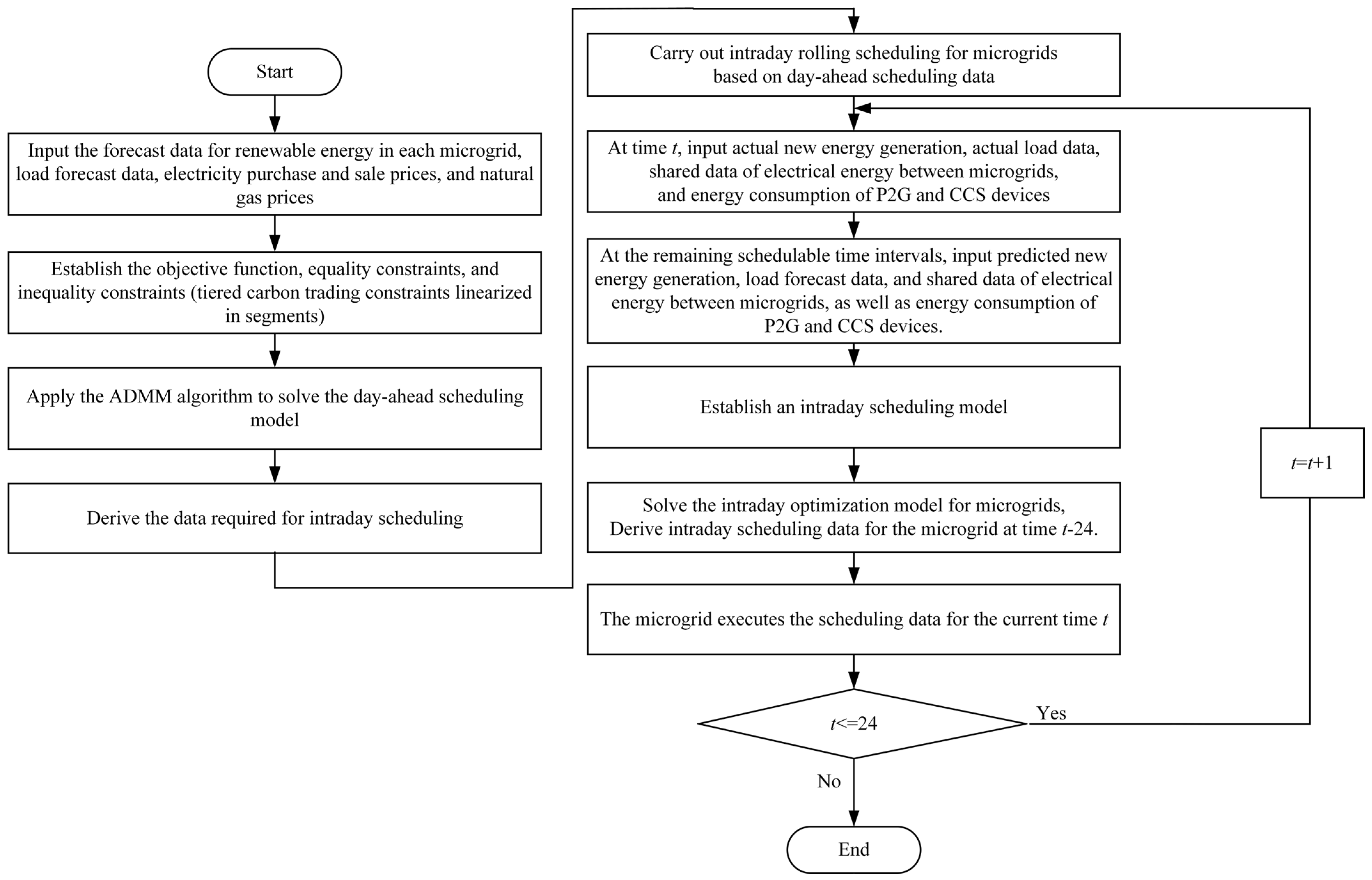
5. The Optimization Strategy for Multi-Microgrids

The strategy for multi-microgrids comprises the day-ahead scheduling stage and the intraday scheduling stage. In the day-ahead scheduling stage, an optimization model is established and solved based on the forecasted values of renewable energy generation and load, taking into account microgrid constraints and carbon emission limitations. This process produces the optimal energy dispatch plan for the next day. In the intraday scheduling stage, an intraday scheduling model is developed, derived from the outcomes of the day-ahead scheduling. This model considers current data on renewable energy generation, the current load, and forecasted information for other time periods, as well as the sharing of electricity between microgrids. Additionally, it incorporates the actual output values of P2G and CCS devices during the optimization period. A rolling optimization strategy is employed to optimize the output of energy devices and the amount of energy purchased, aiming to reduce errors in renewable energy generation and load forecasts. Furthermore, it aims to minimize the penalty costs associated with deviations from the day-ahead plan, ultimately enhancing the economic performance of multi-microgrid operations.

The process of the optimization strategy is illustrated in Figure 4.

5.1. Day-Ahead Optimization Scheduling

5.1.1. The Objective Function

Day-ahead scheduling is aimed at minimizing the total cost of operating the multi-microgrids, with the objective function as follows:

$$\left\{\begin{array}{l}\min {\displaystyle \prod _{i=1}^{\Theta }[C_i^{\mathrm{MG}}]}\\ C_i^{\mathrm{MG}}=C_i^{\mathrm{out}}+C_i^{\mathrm{ESS}}+C_i^{{\mathrm{CO}}_2}+C_i^{\mathrm{load}}+C_i^{\mathrm{cur}}\end{array}\right.$$

(22)

where $\Theta$ is the set of microgrids and $C_i^{\mathrm{MG}}$ is the operating cost of microgrid i.

(1)

The cost of reducing renewable energy output

The cost of reducing renewable energy output in microgrid i, denoted by $C_i^{\mathrm{cur}}$, is calculated using the following Equation (23):

$$C_i^{\mathrm{cur}}={\displaystyle \sum }_{t=1}^T({\lambda }^{\mathrm{cur}}{P}_{i,t}^{\mathrm{cur}})$$

(23)

where ${\lambda }^{\mathrm{cur}}$ is the unit cost of reducing renewable energy output power and $P_{i,t}^{\mathrm{cur}}$ is the reduction power of renewable energy in microgrid i at time t.

(2)

Carbon emission cost

The cost of carbon emission in microgrid i, denoted by $C_i^{{\mathrm{CO}}_2}$, is calculated using the following Equation (24):

$$C_i^{{\mathrm{CO}}_2}={\displaystyle \sum _{\mathrm{t}=1}^{T}C{E}_i^{{\mathrm{CO}}_2}}$$

(24)

(3)

Energy storage cost

The energy storage cost of microgrid i, denoted by $C_i^{\mathrm{ESS}}$, is given by Equation (25), as follows:

$$C_i^{\mathrm{ESS}}={\displaystyle \sum }_{t=1}^T[{\alpha }^{\mathrm{ES}}(P_{i,t}^{\mathrm{ES},\mathrm{c}}+P_{i,t}^{\mathrm{ES},\mathrm{d}})+{\alpha }^{\mathrm{HS}}(P_{i,t}^{\mathrm{HS},\mathrm{c}}+P_{i,t}^{\mathrm{HS},\mathrm{d}})+{\alpha }^{{\mathrm{H}}_2}(P_{i,t}^{\mathrm{H},\mathrm{c}}+P_{i,t}^{\mathrm{H},\mathrm{d}})]$$

(25)

where ${\alpha }^{\mathrm{ES}}$, ${\alpha }^{\mathrm{HS}}$ and ${\alpha }^{{\mathrm{H}}_2}$ are the scheduling cost coefficients for electrical energy, heat energy and hydrogen energy storage, respectively; $P_{i,t}^{\mathrm{ES},\mathrm{c}}$ and $P_{i,t}^{\mathrm{ES},\mathrm{d}}$ are the charging and discharging power of ES in microgrid i during time period t, respectively; $P_{i,t}^{\mathrm{HS},\mathrm{c}}$ and $P_{i,t}^{\mathrm{HS},\mathrm{d}}$ are the charging and discharging power of HS in microgrid i during time period t, respectively; and $P_{i,t}^{\mathrm{H},\mathrm{c}}$ and $P_{i,t}^{\mathrm{H},\mathrm{d}}$ are the charging and discharging power of HSS in microgrid i during time period t, respectively.

(4)

Cost of the load demand

The cost of the load demand in microgrid i, denoted by $C_i^{\mathrm{load}}$, is calculated using the following Equation (26):

$$C_i^{\mathrm{load}}={\displaystyle \sum }_{t=1}^T\left[{\lambda }^{\mathrm{cut},\mathrm{e}}{P}_{i,t}^{\mathrm{e},\mathrm{cut}}+{\lambda }^{\mathrm{trans},\mathrm{e}}{P}_{i,t}^{\mathrm{e},\mathrm{tr}}+{\lambda }^{\mathrm{cut},\mathrm{h}}{P}_{i,t}^{\mathrm{h},\mathrm{cut}}+{\lambda }^{\mathrm{trans},\mathrm{h}}{P}_{i,t}^{\mathrm{h},\mathrm{tr}}\right]$$

(26)

where ${\lambda }^{\mathrm{cut},\mathrm{e}}$ is the compensation coefficient for electric load reduction, ${\lambda }^{\mathrm{cut},\mathrm{h}}$ is the compensation coefficient for heat load reduction, ${\lambda }^{\mathrm{trans},\mathrm{e}}$ is the compensation coefficient for electric load transfer, and ${\lambda }^{\mathrm{trans},\mathrm{h}}$ is the compensation coefficient for heat load transfer.

(5)

External interaction costs

The external interaction costs of microgrid i, denoted by $C_i^{\mathrm{out}}$, mainly consist of two parts; namely, electricity purchase/sale costs and gas purchase costs, which are calculated using the following Equation (27):

$$C_i^{\mathrm{out}}={\displaystyle \sum }_{t=1}^T\left[(M_t^{{\mathrm{CH}}_4}{V}_{i,t}^{\mathrm{BUY}})+(M_t^{\mathrm{BUY}}{P}_{i,t}^{\mathrm{BUY}}-M_t^{\mathrm{SELL}}{P}_{i,t}^{\mathrm{SELL}})\right]$$

(27)

where $M_t^{{\mathrm{CH}}_4}$ is the natural gas price in period t; $V_{i,t}^{\mathrm{BUY}}$ is the natural gas purchase quantity of microgrid i in period t; $P_{i,t}^{\mathrm{BUY}}$ and $P_{i,t}^{\mathrm{SELL}}$ are the purchased and sold power from the grid by microgrid i in the t-th time period, respectively; and $M_t^{\mathrm{BUY}}$ and $M_t^{\mathrm{SELL}}$ are the electricity purchase price and electricity selling price from the grid in period t, respectively.

5.1.2. Constraints

(1)

Electrical power balance constraint

The constraint of electrical power balance is:

$$P_{i,t}^{\mathrm{re}}+P_{i,t}^{\mathrm{e},\mathrm{chp}}+P_{i,t}^{\mathrm{BUY}}+P_{i,t}^{\mathrm{ES},\mathrm{d}}=P_{i,t}^{\mathrm{e},\mathrm{hp}}+P_{i,t}^{\mathrm{e}}+P_{i,t}^{\mathrm{ES},\mathrm{c}}+P_{i,t}^{\mathrm{SELL}}+{\displaystyle \sum _{j\ne i}^{\Theta }{P}_{i-j,t}}+P_{i,t}^{\mathrm{ccssum}}+P_{i,t}^{\mathrm{EL}}$$

(28)

where $P_{i,t}^{\mathrm{re}}$ is the output power of renewable energy in microgrid i at time t; $P_{i-j,t}$ is the amount of electrical energy exchanged between microgrid i and microgrid j in time period t; i ∈ $\Theta$, j ∈ $\Theta$; $P_{i,t}^{\mathrm{e}}$ is the electrical load of microgrid i in the t-th time period, $P_{i,t}^{\mathrm{ES},\mathrm{c}}$ and $P_{i,t}^{\mathrm{ES},\mathrm{d}}$ are the charging and discharging power of the electrical energy storage system in microgrid i in the t-th time period, respectively; and $P_{i,t}^{\mathrm{e},\mathrm{hp}}$ is the electric power consumed by the heat pump in the i-th time period of the microgrid i.

(2)

Heat power balance constraint

The constraint of heat power balance is as follows:

$$P_{i,t}^{\mathrm{h},\mathrm{hp}}+P_{i,t}^{\mathrm{h},\mathrm{chp}}+P_{i,t}^{\mathrm{h},\mathrm{gb}}+P_{i,t}^{\mathrm{HS},\mathrm{d}}=P_{i,t}^{\mathrm{h}}+P_{i,t}^{\mathrm{HS},\mathrm{c}}$$

(29)

where $P_{i,t}^{\mathrm{h}}$ is the heat load of microgrid i at time t; $P_{i,t}^{\mathrm{h},\mathrm{hp}}$ is the heat power generated by the HP in microgrid i at time t; and $P_{i,t}^{\mathrm{HS},\mathrm{c}}$ and $P_{i,t}^{\mathrm{HS},\mathrm{d}}$ are the charging and discharging power of the HS in microgrid i at time t, respectively.

(3)

Gas power balance constraint

The constraint of gas power balance is as follows:

$$\left\{\begin{array}{l}{P}_{i,t}^{\mathrm{g},\mathrm{BUY}}=P_{i,t}^{\mathrm{g},\mathrm{chp}}+P_{i,t}^{\mathrm{g},\mathrm{gb}}-P_{i,t}^{\mathrm{H}2\mathrm{G}, \mathrm{out} }\\ P_{i,t}^{\mathrm{g},\mathrm{BUY}}=V_{i,t}^{\mathrm{BUY}}{Q}_{{\mathrm{CH}}_4}\end{array}\right.$$

(30)

where $P_{i,t}^{\mathrm{g},\mathrm{BUY}}$ is the power of gas purchased externally in microgrid i at time t.

(4)

Hydrogen power balance constraint

The constraint of hydrogen power balance is as follows:

$$P_{i,t}^{\mathrm{EL},{\mathrm{H}}_2}+P_{i,t}^{\mathrm{H},\mathrm{d}}=P_{i,t}^{{\mathrm{h}}_2,\mathrm{chp}}+P_{i,t}^{{\mathrm{h}}_2,\mathrm{gb}}+P_{i,t}^{\mathrm{H},\mathrm{c}}+P_{i,t}^{\mathrm{H}2\mathrm{G}, \mathrm{in} }$$

(31)

(5)

Renewable energy supply constraint

The constraint of renewable energy is as follows:

$$\left\{\begin{array}{l}{P}_{i,t}^{\mathrm{e},\mathrm{r}}=P_{i,t}^{\mathrm{cur}}+P_{i,t}^{\mathrm{re}}\hfill \\ 0\le P_{i,t}^{\mathrm{re}}\le P_{i,t}^{\mathrm{e},\mathrm{r}}\hfill \end{array}\right.$$

(32)

The actual renewable energy output is seen as the aggregate of the predicted value and the stochastic forecasting error. The prediction error of renewable energy output follows a normal distribution, and it is expressed in Equation (33), as follows [31]:

$$P_{i,t}^{\mathrm{e},\mathrm{r}}~{\overline{P}}_{i,t}^{\mathrm{e},\mathrm{r}}+N(0,{\sigma }_{i,t}^2)$$

(33)

where $P_{i,t}^{\mathrm{e},\mathrm{r}}$ is the actual renewable energy generation power; ${\overline{P}}_{i,t}^{\mathrm{e},\mathrm{r}}$ is the predicted renewable energy generation power; and ${\sigma }_{i,t}^2$ is the variance of renewable energy generation, =0.1.

(6)

Hydrogen energy storage system constraint

The constraint of the HSS is as follows:

$$\left\{\begin{array}{l}{E}_{i,t}^{{\mathrm{H}}_2}=E_{i,t-1}^{{\mathrm{H}}_2}+{\eta }_i^{\mathrm{H},\mathrm{c}}{P}_{i,t}^{\mathrm{H},\mathrm{c}}\Delta t-\frac{P_{i,t}^{\mathrm{H},\mathrm{d}}\Delta t}{{\eta }_i^{\mathrm{H},\mathrm{d}}}\hfill \\ E_{i,0}^{{\mathrm{H}}_2}=E_{i,T}^{{\mathrm{H}}_2}\hfill \\ E_{i,\min }^{{\mathrm{H}}_2}\le E_{i,t}^{{\mathrm{H}}_2}\le E_{i,\max }^{{\mathrm{H}}_2}\hfill \\ 0\le P_{i,t}^{\mathrm{H},\mathrm{c}}\le u_t^{\mathrm{H},\mathrm{c}}{P}_{i,\max }^{\mathrm{H},\mathrm{c}}\hfill \\ 0\le P_{i,t}^{\mathrm{H},\mathrm{d}}\le u_t^{\mathrm{H},\mathrm{d}}{P}_{i,\max }^{\mathrm{H},\mathrm{d}}\hfill \\ 0\le u_t^{\mathrm{H},\mathrm{d}}+u_t^{\mathrm{H},\mathrm{c}}\le 1\hfill \end{array}\right.$$

(34)

In Equation (34), $E_{i,t}^{{\mathrm{H}}_2}=E_{i,t-1}^{{\mathrm{H}}_2}+{\eta }_i^{\mathrm{H},\mathrm{c}}{P}_{i,t}^{\mathrm{H},\mathrm{c}}\Delta t-\frac{P_{i,t}^{\mathrm{H},\mathrm{d}}\Delta t}{{\eta }_i^{\mathrm{H},\mathrm{d}}}$ is the conversion formula for hydrogen energy storage capacity and $E_{i,0}^{{\mathrm{H}}_2}=E_{i,T}^{{\mathrm{H}}_2}$ indicates that the stored energy of the HSS is the same after the optimization period ends. $E_{i,\min }^{{\mathrm{H}}_2}\le E_{i,t}^{{\mathrm{H}}_2}\le E_{i,\max }^{{\mathrm{H}}_2}$ is the constraint on hydrogen energy storage capacity. $0\le P_{i,t}^{\mathrm{H},\mathrm{c}}\le u_t^{\mathrm{H},\mathrm{c}}{P}_{i,\max }^{\mathrm{H},\mathrm{c}}$ and $0\le P_{i,t}^{\mathrm{H},\mathrm{d}}\le u_t^{\mathrm{H},\mathrm{d}}{P}_{i,\max }^{\mathrm{H},\mathrm{d}}$ are the constraints on the power of energy storage and discharge in hydrogen storage, respectively. $0\le u_t^{\mathrm{H},\mathrm{d}}+u_t^{\mathrm{H},\mathrm{c}}\le 1$ indicates that energy storage and discharge cannot occur simultaneously. $E_{i,t}^{{\mathrm{H}}_2}$ is the hydrogen storage of the HSS in microgrid i at time t; ${\eta }_i^{\mathrm{H},\mathrm{c}}$ and ${\eta }_i^{\mathrm{H},\mathrm{d}}$ are the charging and the discharging efficiency of the hydrogen energy storage device in the microgrid i; and $E_{i,\min }^{{\mathrm{H}}_2}$ and $E_{i,\max }^{{\mathrm{H}}_2}$ are the minimum and maximum storage capacity of the HSS in the microgrid i, respectively. The binary variables $u_t^{\mathrm{H},\mathrm{d}}$ and $u_t^{\mathrm{H},\mathrm{c}}$ indicate that hydrogen storage and hydrogen discharge cannot occur simultaneously.

(7)

Electrical energy storage system constraint

The ES in microgrid i during the t-th time period is formulated as follows:

$$\left\{\begin{array}{l}\begin{array}{l}{E}_{i,t}^{\mathrm{ES}}=E_{i,t-1}^{\mathrm{ES}}+{\eta }_i^{\mathrm{ES},\mathrm{c}}{P}_{i,t}^{\mathrm{ES},\mathrm{c}}\Delta t-\frac{P_{i,t}^{\mathrm{ES},\mathrm{d}}\Delta t}{{\eta }_i^{\mathrm{ES},\mathrm{d}}}\\ E_{i,0}^{\mathrm{ES}}=E_{i,T}^{\mathrm{ES}}\end{array}\hfill \\ E_{i,\min }^{\mathrm{ES}}\le E_{i,t}^{\mathrm{ES}}\le E_{i,\max }^{\mathrm{ES}}\hfill \\ 0\le P_{i,t}^{\mathrm{ES},\mathrm{c}}\le u_t^{\mathrm{ES},\mathrm{c}}{P}_{i,\max }^{\mathrm{ES},\mathrm{c}}\hfill \\ 0\le P_{i,t}^{\mathrm{ES},\mathrm{d}}\le u_t^{\mathrm{ES},\mathrm{d}}{P}_{i,\max }^{\mathrm{ES},\mathrm{d}}\hfill \\ 0\le u_t^{\mathrm{ES},\mathrm{c}}+u_t^{\mathrm{ES},\mathrm{d}}\le 1\hfill \end{array}\right.$$

(35)

In Equation (35), $E_{i,t}^{\mathrm{ES}}=E_{i,t-1}^{\mathrm{ES}}+{\eta }_i^{\mathrm{ES},\mathrm{c}}{P}_{i,t}^{\mathrm{ES},\mathrm{c}}\Delta t-\frac{P_{i,t}^{\mathrm{ES},\mathrm{d}}\Delta t}{{\eta }_i^{\mathrm{ES},\mathrm{d}}}$ is the conversion relationship formula for electrical energy storage capacity and $E_{i,0}^{\mathrm{ES}}=E_{i,T}^{\mathrm{ES}}$ indicates that the energy stored in the ES is the same after the entire optimization scheduling period. $E_{i,\min }^{\mathrm{ES}}\le E_{i,t}^{\mathrm{ES}}\le E_{i,\max }^{\mathrm{ES}}$ is the constraint on electrical energy storage capacity. $0\le P_{i,t}^{\mathrm{ES},\mathrm{c}}\le u_t^{\mathrm{ES},\mathrm{c}}{P}_{i,\max }^{\mathrm{ES},\mathrm{c}}$ and $0\le P_{i,t}^{\mathrm{ES},\mathrm{d}}\le u_t^{\mathrm{ES},\mathrm{d}}{P}_{i,\max }^{\mathrm{ES},\mathrm{d}}$ are the constraints on the power of energy storage and discharge in ES, respectively. $0\le u_t^{\mathrm{ES},\mathrm{c}}+u_t^{\mathrm{ES},\mathrm{d}}\le 1$ indicates that energy storage and discharge cannot occur simultaneously. $E_{i,t}^{\mathrm{ES}}$ is the electrical energy storage capacity in the ES of microgrid i in the t-th time period; ${\eta }_i^{\mathrm{ES},\mathrm{c}}$ and ${\eta }_i^{\mathrm{ES},\mathrm{d}}$ are the charging and discharging efficiency of the ES in microgrid i, respectively; $E_{i,\min }^{\mathrm{ES}}$ and $E_{i,\max }^{\mathrm{ES}}$ are the minimum and maximum storage capacity of the ES in microgrid i, respectively; and $P_{i,\max }^{\mathrm{ES},\mathrm{c}}$ and $P_{i,\max }^{\mathrm{ES},\mathrm{d}}$ are the maximum charging and discharging power of the ES in microgrid i, respectively. The two binary variables $u_t^{\mathrm{ES},\mathrm{c}}$ and $u_t^{\mathrm{ES},\mathrm{d}}$ indicate that charging and discharging cannot occur simultaneously.

(8)

Heat energy storage constraint

The constraint of HS is as follows:

$$\left\{\begin{array}{l}{E}_{i,t}^{\mathrm{HS}}=E_{i,t-1}^{\mathrm{HS}}+{\eta }_i^{\mathrm{HS},\mathrm{c}}{P}_{i,t}^{\mathrm{HS},\mathrm{c}}\Delta t-\frac{P_{i,t}^{\mathrm{HS},\mathrm{d}}\Delta t}{{\eta }_i^{\mathrm{HS},\mathrm{d}}}\\ \begin{array}{l}{E}_{i,0}^{\mathrm{HS}}=E_{i,T}^{\mathrm{HS}}\hfill \\ E_{i,\min }^{\mathrm{HS}}\le E_{i,t}^{\mathrm{HS}}\le E_{i,\max }^{\mathrm{HS}}\hfill \\ 0\le P_{i,t}^{\mathrm{HS},\mathrm{c}}\le u_t^{\mathrm{HS},\mathrm{c}}{P}_{i,\max }^{\mathrm{HS},\mathrm{c}}\hfill \\ 0\le P_{i,t}^{\mathrm{HS},\mathrm{d}}\le u_t^{\mathrm{HS},\mathrm{d}}{P}_{i,\max }^{\mathrm{HS},\mathrm{d}}\hfill \\ 0\le u_t^{\mathrm{HS},\mathrm{d}}+u_t^{\mathrm{HS},\mathrm{c}}\le 1\hfill \end{array}\end{array}\right.$$

(36)

In Equation (36), $E_{i,t}^{\mathrm{HS}}=E_{i,t-1}^{\mathrm{HS}}+{\eta }_i^{\mathrm{HS},\mathrm{c}}{P}_{i,t}^{\mathrm{HS},\mathrm{c}}\Delta t-\frac{P_{i,t}^{\mathrm{HS},\mathrm{d}}\Delta t}{{\eta }_i^{\mathrm{HS},\mathrm{d}}}$ is the conversion relationship formula for heat energy storage capacity and $E_{i,0}^{\mathrm{HS}}=E_{i,T}^{\mathrm{HS}}$ indicates that the heat energy storage capacity of the HS is the same after the optimization period ends. $E_{i,\min }^{\mathrm{HS}}\le E_{i,t}^{\mathrm{HS}}\le E_{i,\max }^{\mathrm{HS}}$ is the constraint on heat energy storage capacity. $0\le P_{i,t}^{\mathrm{HS},\mathrm{c}}\le u_t^{\mathrm{HS},\mathrm{c}}{P}_{i,\max }^{\mathrm{HS},\mathrm{c}}$ and $0\le P_{i,t}^{\mathrm{HS},\mathrm{d}}\le u_t^{\mathrm{HS},\mathrm{d}}{P}_{i,\max }^{\mathrm{HS},\mathrm{d}}$ are the constraints on the power of energy storage and discharge in heat storage, respectively. $0\le u_t^{\mathrm{HS},\mathrm{d}}+u_t^{\mathrm{HS},\mathrm{c}}\le 1$ indicates that energy storage and discharge cannot occur simultaneously. $E_{i,t}^{\mathrm{HS}}$ is the energy stored in the HS of microgrid i in the t-th time period; ${\eta }_i^{\mathrm{HS},\mathrm{c}}$ and ${\eta }_i^{\mathrm{HS},\mathrm{d}}$ are the charging and discharging efficiency of the HS in microgrid i, respectively; and $P_{i,\max }^{\mathrm{HS},\mathrm{c}}$ and $P_{i,\max }^{\mathrm{HS},\mathrm{d}}$ are the maximum charging and discharging power of the HS in microgrid i, respectively.

(9)

Heat pump constraint

The constraint of HP is as follows:

$$\left\{\begin{array}{l}{P}_{i,t}^{\mathrm{h},\mathrm{hp}}={\eta }_i^{\mathrm{hp}}{P}_{i,t}^{\mathrm{e},\mathrm{hp}}\\ P_{i,\min }^{\mathrm{e},\mathrm{hp}}\le P_{i,t}^{\mathrm{e},\mathrm{hp}}\le P_{i,\max }^{\mathrm{e},\mathrm{hp}}\end{array}\right.$$

(37)

In Equation (37), $P_{i,t}^{\mathrm{h},\mathrm{hp}}={\eta }_i^{\mathrm{hp}}{P}_{i,t}^{\mathrm{e},\mathrm{hp}}$ is the power conversion relationship between electricity and heat in the HP and $P_{i,\min }^{\mathrm{e},\mathrm{hp}}\le P_{i,t}^{\mathrm{e},\mathrm{hp}}\le P_{i,\max }^{\mathrm{e},\mathrm{hp}}$ is the electrical power constraint relationship in the HP. ${\eta }_i^{\mathrm{hp}}$ is the electrical-to-heat conversion efficiency of the HP in the microgrid i. $P_{i,\min }^{\mathrm{e},\mathrm{hp}}$ and $P_{i,\max }^{\mathrm{e},\mathrm{hp}}$ are the minimum and maximum electric power consumption of the HP in microgrid i, respectively.

(10)

The constraints between the microgrid and power grid

The constraint between the microgrid and power grid is as follows:

$$\left\{\begin{array}{c}0\le P_{i,t}^{\mathrm{BUY}}\le P_{i,\max }^{\mathrm{BUY}}\\ 0\le P_{i,t}^{\mathrm{SELL}}\le P_{i,\max }^{\mathrm{SELL}}\end{array}\right.$$

(38)

In Equation (38), $0\le P_{i,t}^{\mathrm{BUY}}\le P_{i,\max }^{\mathrm{BUY}}$ and $0\le P_{i,t}^{\mathrm{SELL}}\le P_{i,\max }^{\mathrm{SELL}}$ are the constraints on purchasing electricity from the grid and selling electricity to the grid, respectively. $P_{i,\max }^{\mathrm{BUY}}$ and $P_{i,\max }^{\mathrm{SELL}}$ are the upper limits of power bought from and sold to the grid in microgrid i.

(11)

Electrical and heat load constraints

The electrical load of microgrid i at time t, denoted by $P_{i,t}^{\mathrm{e}}$ is composed of the following: the fixed electrical load, $P_{i,t}^{\mathrm{e},\mathrm{g}}$; the transferable electrical load, $P_{i,t}^{\mathrm{e},\mathrm{tr}}$; and the reducible electrical load, $P_{i,t}^{\mathrm{e},\mathrm{cut}}$. The relationship is modeled as follows:

$$\left\{\begin{array}{l}{P}_{i,t}^{\mathrm{e}}=P_{i,t}^{\mathrm{e},\mathrm{g}}+P_{i,t}^{\mathrm{e},\mathrm{tr}}-P_{i,t}^{\mathrm{e},\mathrm{cut}}\hfill \\ -a^{\mathrm{tr}}{P}_{i,t}^{\mathrm{e},\mathrm{g}}\le P_{i,t}^{\mathrm{e},\mathrm{tr}}\le a^{\mathrm{tr}}{P}_{i,t}^{\mathrm{e},\mathrm{g}}\hfill \\ 0\le P_{i,t}^{\mathrm{e},\mathrm{cut}}\le b^{\mathrm{cut}}{P}_{i,t}^{\mathrm{e},\mathrm{f}}\hfill \\ {\displaystyle \sum _{t=1}^T{P}_{i,t}^{\mathrm{e},\mathrm{tr}}}=0\hfill \end{array}\right.$$

(39)

In Equation (39), $-a^{\mathrm{tr}}{P}_{i,t}^{\mathrm{e},\mathrm{g}}\le P_{i,t}^{\mathrm{e},\mathrm{tr}}\le a^{\mathrm{tr}}{P}_{i,t}^{\mathrm{e},\mathrm{g}}$ and $0\le P_{i,t}^{\mathrm{e},\mathrm{cut}}\le b^{\mathrm{cut}}{P}_{i,t}^{\mathrm{e},\mathrm{f}}$ are the constraints on transferred and curtailable electrical loads. ${\displaystyle \sum _{t=1}^T{P}_{i,t}^{\mathrm{e},\mathrm{tr}}}=0$ indicates no loss of transferable load during the dispatch cycle. $a^{\mathrm{tr}}$ is the transfer load coefficient and $b^{\mathrm{cut}}$ is the reducible load coefficient.

The heat load of microgrid i at time t, denoted by $P_{i,t}^{\mathrm{h}}$, is composed of the following: the fixed heat load, $P_{i,t}^{\mathrm{h},\mathrm{g}}$; the transferable heat load, $P_{i,t}^{\mathrm{h},\mathrm{tr}}$; and the reducible heat load, $P_{i,t}^{\mathrm{h},\mathrm{cut}}$. The relationship is modeled as follows:

$$\left\{\begin{array}{l}{P}_{i,t}^{\mathrm{h}}=P_{i,t}^{\mathrm{h},\mathrm{g}}+P_{i,t}^{\mathrm{h},\mathrm{tr}}-P_{i,t}^{\mathrm{h},\mathrm{cut}}\hfill \\ -a^{\mathrm{tr}}{P}_{i,t}^{\mathrm{h},\mathrm{g}}\le P_{i,t}^{\mathrm{h},\mathrm{tr}}\le a^{\mathrm{tr}}{P}_{i,t}^{\mathrm{h},\mathrm{g}}\hfill \\ 0\le P_{i,t}^{\mathrm{h},\mathrm{cut}}\le b^{\mathrm{cut}}{P}_{i,t}^{\mathrm{h},\mathrm{f}}\hfill \\ {\displaystyle \sum _{t=1}^T{P}_{i,t}^{\mathrm{h},\mathrm{tr}}}=0\hfill \end{array}\right.$$

(40)

In Equation (40), $-a^{\mathrm{tr}}{P}_{i,t}^{\mathrm{h},\mathrm{g}}\le P_{i,t}^{\mathrm{h},\mathrm{tr}}\le a^{\mathrm{tr}}{P}_{i,t}^{\mathrm{h},\mathrm{g}}$ and $0\le P_{i,t}^{\mathrm{h},\mathrm{cut}}\le b^{\mathrm{cut}}{P}_{i,t}^{\mathrm{h},\mathrm{f}}$ are the constraints on transferred and curtailable heat loads. ${\displaystyle \sum _{t=1}^T{P}_{i,t}^{\mathrm{h},\mathrm{tr}}}=0$ indicates no loss of transferable load during the dispatch cycle.

(12)

Constraint of energy transfer between microgrids

The constraint of energy transfer between microgrids is as follows:

$$\left|P_{i-j,t}\right|\le P_{i-j,\max }$$

(41)

where $P_{i-j,\max }$ is the limitation on power transfer between microgrid i and microgrid j. The other constraints are described by Equations (1)–(21).

5.1.3. Model Linearization and Solution

The day-ahead model, integrating tiered carbon trading mechanisms, P2G–CCS coupling technology and gas hydrogenation technology, require linearization due to their mixed-integer non-linear nature.

Equation (20) is linearized by introducing 0–1 variables, and the linearization of the piecewise function is expressed as follows [28]:

$$y=\left\{\begin{array}{ll}{a}_{1}x+b_1,\hfill & c_1\le x\le c_2\hfill \\ a_{2}x+b_2,\hfill & c_2\le x\le c_3\hfill \\ a_{3}x+b_3,\hfill & c_3\le x\le c_4\hfill \end{array}\right.$$

(42)

By introducing binary variables, denoted by $d_i$, and continuous variables, denoted by $z_i$, the original Equation (42) is transformed into Equation (43), to impose interval constraints on the values of x and b. This step ensures that the values of variables x and b are limited to specific single intervals, enhancing the accuracy and applicability of the mathematical model.

$$\left\{\begin{array}{l}y={\displaystyle \sum _i^3{a}_i}{z}_i+b_i{d}_i\\ x=z_1+z_2+z_3\\ d_1+d_2+d_3=1\\ d_1{c}_1\le a_1{z}_1\le d_1{c}_2\\ d_2{c}_2\le a_2{z}_2\le d_2{c}_3\\ d_3{c}_3\le a_3{z}_3\le d_3{c}_4\end{array}\right.$$

(43)

5.1.4. Model Solution

The alternating direction method of multipliers (ADMM) is applied to solve the day-ahead scheduling model by taking the following steps:

(1)

Introduce auxiliary variables, $P_{j-i,t}$, to construct auxiliary expressions, as follows:

$$P_{i-j,t}+P_{j-i,t}=0,\forall i$$

(44)

where $P_{j-i,t}$ is the amount of electrical energy exchanged between microgrid j and microgrid i in time period t.

(2)

Formulate the augmented Lagrangian function expression for the day-ahead issue, as follows:

$$\left\{\begin{array}{l}{L}_i=\min [C_i^{\mathrm{MG}}]+{\displaystyle \sum _j^{\Theta }}{\displaystyle \sum _{t=1}^T}{\lambda }_{i-j}\left(P_{i-j,t}+P_{j-i,t}\right)+{\displaystyle \sum _j^{\Theta }}\frac{{\rho }_i}{2}{\displaystyle \sum _{t=1}^T}||P_{i-j,t}+P_{j-i,t}|{|}_2^2\\ \mathrm{s}.\mathrm{t}.\left(1\right)–\left(21\right), \left(28\right)–\left(43\right)\end{array}\right.$$

(45)

where ${\lambda }_{i-j}$ is the Lagrange multiplier and ${\rho }_i(k)$ is the penalty parameter at the k-th iteration.

(3)

Initialize the iteration number k = 1 and iterate through the following steps:

Update the decision variables for the microgrid, $P_{i-j,t}(k+1)$, as follows:

$$P_{i-j,t}(k+1)=\arg \min L_i({\lambda }_{i-j}(k),P_{i-j,t}(k),P_{j-i,t}(k))$$

(46)

Based on the variable $P_{i-j,t}(k+1)$, microgrid j updates its decision variables $P_{j-i,t}(k+1)$ through Equation (47), as follows:

$$P_{j-i,t}(k+1)=\arg \min L_j({\lambda }_{j-i}(k),P_{i-j,t}(k+1),P_{j-i,t}(k))$$

(47)

Each microgrid updates its variables in each iteration process.

(4)

Update the Lagrange multiplier parameters after each iteration, as follows:

$${\lambda }_{i-j}(k+1)={\lambda }_{i-j}(k)+{\rho }_i(k)(P_{i-j,t}+P_{j-i,t})$$

(48)

(5)

Determine the convergence of the algorithm, as follows:

$$\left\{\begin{array}{c}{\displaystyle \sum _{t=1}^T{\displaystyle \sum _{i=1}^{\Theta }{‖P_{i-j,t}(k+1)+P_{j-i,t}(k+1)‖}_2}}\le {\epsilon }^{\mathrm{pri}}\\ {\displaystyle \sum _{t=1}^T{\displaystyle \sum _{i=1}^{\Theta }{‖P_{i-j,t}(k+1)-P_{i-j,t}(k)‖}_2}}\le {\epsilon }^{\mathrm{dual}}\end{array}\right.$$

(49)

where ${\epsilon }^{\mathrm{pri}}$ denotes the primal residuals and ${\epsilon }^{\mathrm{dual}}$ denotes the dual residuals.

If the convergence condition of Equation (49) or k > k_max is satisfied, the iteration terminates; otherwise, update the iteration number to k + 1 and update the penalty parameter, repeating steps (3)–(5).

5.2. Intraday Optimization Scheduling

The objective expression for the intraday dispatch of microgrids is as follows:

$$\min \{{\overline{C}}_i^{\mathrm{cur}}+{\overline{C}}_i^{\mathrm{outer}}+{\overline{C}}_i^{\mathrm{ESS}}+{\overline{C}}_i^{{\mathrm{CO}}_2}+{\overline{C}}_i^{\mathrm{pun}}\}$$

(50)

where:

$$\begin{array}{l}{\overline{C}}_i^{\mathrm{pun}}=\hfill \\ {\displaystyle \sum _{\tau \in T_{\mathrm{S}}}}{\lambda }^{\mathrm{p}}\left[\begin{array}{c}\begin{array}{l}({\overline{P}}_{i,\tau }^{\mathrm{e},\mathrm{chp}}-{\widehat{P}}_{i,\tau }^{\mathrm{e},\mathrm{chp}}{)}^2+({\overline{P}}_{i,\tau }^{\mathrm{h},\mathrm{gb}}-{\widehat{P}}_{i,\tau }^{\mathrm{h},\mathrm{gb}}{)}^2+({\overline{P}}_{i,\tau }^{\mathrm{ES},\mathrm{c}}-{\widehat{P}}_{i,\tau }^{\mathrm{ES},\mathrm{c}}{)}^2+({\overline{P}}_{i,\tau }^{\mathrm{ES},\mathrm{d}}-{\widehat{P}}_{i,\tau }^{\mathrm{ES},\mathrm{d}}{)}^2\\ +({\overline{P}}_{i,\tau }^{\mathrm{HS},\mathrm{c}}-{\widehat{P}}_{i,\tau }^{\mathrm{HS},\mathrm{c}}{)}^2+({\overline{P}}_{i,\tau }^{\mathrm{HS},\mathrm{d}}-{\widehat{P}}_{i,\tau }^{\mathrm{HS},\mathrm{d}}{)}^2+({\overline{P}}_{i,\tau }^{\mathrm{SELL}}-{\widehat{P}}_{i,\tau }^{\mathrm{SELL}}{)}^2+({\overline{P}}_{i,\tau }^{\mathrm{BUY}}-{\widehat{P}}_{i,\tau }^{\mathrm{BUY}}{)}^2\\ +({\overline{V}}_{i,\tau }^{\mathrm{BUY}}-{\widehat{V}}_{i,\tau }^{\mathrm{BUY}}{)}^2+({\overline{P}}_{i,\tau }^{\mathrm{hp}}-{\widehat{P}}_{i,\tau }^{\mathrm{hp}}{)}^2+({\overline{P}}_{i,t}^{\mathrm{H},\mathrm{d}}-{\widehat{P}}_{i,t}^{\mathrm{H},\mathrm{d}}{)}^2+({\overline{P}}_{i,t}^{\mathrm{H},\mathrm{c}}-{\widehat{P}}_{i,t}^{\mathrm{H},\mathrm{c}}{)}^2\end{array}\end{array}\right]\hfill \end{array}$$

(51)

In Equation (51), $(\overline{•})$ and $(\widehat{•})$ are the day-ahead and intraday variables and ${\lambda }^{\mathrm{p}}$ is the unit penalty cost coefficient. $T_{\mathrm{S}}$ is the intraday optimization scheduling horizon at time t, $T_{\mathrm{S}}=\{t,t+1,\dots ,T\}$.

During the intraday dispatch phase, the rolling optimization process proceeds as follows: Based on the actual values of renewable energy output and load at time t and their predicted values for the remaining time, the rolling optimization model within the intraday time domain is solved to obtain the optimal solution. The microgrid executes the optimization solution in time domain t, and the process is repeated for the next scheduling cycle at time t + 1. The intraday dispatch adjusts the solution derived from the outcomes of the day-ahead optimization dispatch, utilizing the electricity power sharing data between microgrids obtained from the day-ahead stage, as well as the actual load values forecasted beforehand.

Some constraints in the intraday stage are derived from the day-ahead stage, such as constraints (1)–(21), (32)–(38) and (42)–(43); different constraints in the intraday stage are calculated as follows:

$$\begin{array}{l}{\overline{P}}_{i,\tau }^{\mathrm{re}}+{\overline{P}}_{i,\tau }^{\mathrm{e},\mathrm{chp}}+{\overline{P}}_{i,\tau }^{\mathrm{BUY}}+{\overline{P}}_{i,\tau }^{\mathrm{ES},\mathrm{d}}=\\ {\overline{P}}_{i,\tau }^{\mathrm{e},\mathrm{hp}}+{\overline{P}}_{i,\tau }^{\mathrm{SELL}}+{\overline{P}}_{i,\tau }^{\mathrm{ES},\mathrm{c}}+{\overline{P}}_{i,\tau }^{\mathrm{e}}+\Delta {\overline{P}}_{i,\tau }^{\mathrm{e}}+{\displaystyle \sum _{j\ne i}^{\Theta }{\widehat{P}}_{i-j,\tau }+{\widehat{P}}_{i,t}^{\mathrm{ccssum}}+{\widehat{P}}_{i,t}^{\mathrm{EL}},\forall \tau \in T_{\mathrm{S}},\forall i\in \Theta }\end{array}$$

(52)

$${\overline{P}}_{i,\tau }^{\mathrm{h},\mathrm{hp}}+{\overline{P}}_{i,\tau }^{\mathrm{h},\mathrm{chp}}+{\overline{P}}_{i,\tau }^{\mathrm{h},\mathrm{gb}}+{\overline{P}}_{i,\tau }^{\mathrm{HS},\mathrm{d}}={\overline{P}}_{i,\tau }^{\mathrm{HS},\mathrm{c}}+{\overline{P}}_{i,\tau }^{\mathrm{h}}+\Delta {\overline{P}}_{i,\tau }^{\mathrm{h}},\forall \tau \in T_{\mathrm{S}},\forall i\in \Theta$$

(53)

$${\overline{P}}_{i,t}^{\mathrm{g},\mathrm{BUY}}={\overline{P}}_{i,t}^{\mathrm{g},\mathrm{chp}}+{\overline{P}}_{i,t}^{\mathrm{g},\mathrm{gb}}-{\overline{P}}_{i,t}^{\mathrm{H}2\mathrm{G}, \mathrm{out} },\forall \tau \in T_{\mathrm{S}},\forall i\in \Theta$$

(54)

$${\overline{P}}_{i,t}^{\mathrm{EL},{\mathrm{H}}_2}+{\overline{P}}_{i,t}^{\mathrm{H},\mathrm{d}}={\overline{P}}_{i,t}^{{\mathrm{h}}_2,\mathrm{chp}}+{\overline{P}}_{i,t}^{{\mathrm{h}}_2,\mathrm{gb}}+{\overline{P}}_{i,t}^{\mathrm{H},\mathrm{c}}+{\overline{P}}_{i,t}^{\mathrm{H}2\mathrm{G}, \mathrm{in} },\forall \tau \in T_{\mathrm{S}},\forall i\in \Theta$$

(55)

In Equations (52) and (53), $\Delta {\overline{P}}_{i,\tau }^{\mathrm{e}}$ is the discrepancy between the actual and forecasted electrical load values of microgrid i at time t, and $\Delta {\overline{P}}_{i,\tau }^{\mathrm{h}}$ is the discrepancy between the actual and forecasted heat load values of microgrid i at time t.

6. Experimental Verification

6.1. Parameter Settings

The multi-microgrids model in this chapter consists of three microgrids, denoted as microgrid 1, 2, and 3 (MG1, MG2, and MG3), each equipped with hydrogen blending units, carbon capture, and a two-stage P2G unit. The pricing for electricity purchase and sale transactions between the microgrids and the grid is displayed in

Table 1. Electricity purchase and sale price chart.

Category	Time Period	Price ((CNY)/kWh)
Electricity price	23:00–7:00	0.40
	08:00–11:00, 15:00–18:00	0.75
	12:00–14:00, 19:00–22.00	1.20
Electricity sale	0:00–24:00	0.20

. The microgrid system parameters are detailed in

Table 2. Microgrid parameters.

Parameter	Value	Parameter	Value	Parameter	Value
$P_{i,\min }^{\mathrm{e},\mathrm{chp}}$ (kW)	0	$P_{i,\min }^{\mathrm{HS},\mathrm{c} }$ (kW)	0	${\eta }_i^{\mathrm{e},\mathrm{chp}}$	0.3
$P_{i,\max }^{\mathrm{e},\mathrm{chp}}$ (kW)	2000	$P_{i,\max }^{\mathrm{HS},\mathrm{c} }$ (kW)	300	$Q_{{\mathrm{CH}}_4}$	9.7
$P_{i,\min }^{\mathrm{h},\mathrm{chp}}$ (kW)	0	$P_{i,\max }^{\mathrm{HS},\mathrm{d}}$ (kW)	300	$Q_{{\mathrm{H}}_2}$	3.55
$P_{i,\max }^{\mathrm{h},\mathrm{chp}}$ (kW)	2000	$P_{i,\min }^{\mathrm{HS},\mathrm{d}}$ (kW)	0	$D^{\mathrm{chp}}$	0.01
$P_{i,\max }^{\mathrm{ccs}}$ (kW)	1700	$E_{i,\min }^{\mathrm{HS}}$ (kWh)	200	$D^{\mathrm{gb}}$	0.01
$P_{i,t}^{\mathrm{b}}$ (kW)	300	$E_{i,\max }^{\mathrm{HS}}$ (kWh)	1200	$D^{\mathrm{res}}$	0.01
$P_{i,\min }^{\mathrm{ccssum}}$ (kW)	0	$E_{i,\min }^{{\mathrm{H}}_2}$ (kWh)	200	$a^{{\mathrm{co}}_2}$	0.5
$P_{i,\min }^{\mathrm{ccssum}}$ (kW)	2000	$E_{i,\max }^{{\mathrm{H}}_2}$ (kWh)	1200	$b^{{\mathrm{co}}_2}$	0.65
$P_{i,\max }^{\mathrm{h},\mathrm{gb}}$ (kW)	2000	${\eta }_i^{{\mathrm{H}}_2\left(\mathrm{c}\right)}$	0.95	$c^{{\mathrm{co}}_2}$	18.20
${\lambda }_{i,\min }^{\mathrm{e},\mathrm{chp}}$ (kW)	−1000	${\eta }_i^{{\mathrm{H}}_2,\mathrm{d}}$	0.95	${\lambda }_{\mathrm{e}}$	0.2
${\lambda }_{i,\max }^{\mathrm{e},\mathrm{chp}}$ (kW)	1000	$P_{i,\max }^{{\mathrm{H}}_2,\mathrm{c} }$ (kW)	300	${\eta }_i^{\mathrm{C}}$	0.9
${\lambda }_{i,\min }^{\mathrm{h},\mathrm{gb}}$ (kW)	−1000	$P_{i,\max }^{{\mathrm{H}}_2,\mathrm{d}}$ (kW)	300	${\sigma }_{\mathrm{c}}$	0.1
${\lambda }_{i,\max }^{\mathrm{h},\mathrm{gb}}$ (kW)	1000	$P_{i,\min }^{\mathrm{EL}}$ (kW)	0	${\eta }_i^{\mathrm{hp}}$	0.35
$P_{i,\min }^{\mathrm{e},\mathrm{hp}}$ (kW)	0	$P_{i,\max }^{\mathrm{EL}}$ (kW)	1500	${\eta }_i^{\mathrm{gb}}$	0.9
$P_{i,\max }^{\mathrm{e},\mathrm{hp}}$ (kW)	1000	$P_{i,\mathrm{d}}^{\mathrm{EL}}$ (kW)	−300	${\eta }_{\min }^{\mathrm{soc}}$	0.2
$P_{i,\min }^{\mathrm{ES},\mathrm{c}}$ (kW)	0	$P_{i,\mathrm{up}}^{\mathrm{EL}}$ (kW)	300	${\eta }_{\max }^{\mathrm{soc}}$	0.9
$P_{i,\max }^{\mathrm{ES},\mathrm{c} }$ (kW)	300	$P_{i,\max }^{\mathrm{buy}}$ (kWh)	1800	$C_i^{\mathrm{rate}}$	2000
$P_{i,\min }^{\mathrm{ES},\mathrm{d}}$ (kW)	0	$V_i^{\mathrm{CR}}$ (m3)	100,000	${\eta }_i^{\mathrm{EL}}$	0.85
$P_{i,\max }^{\mathrm{ES},\mathrm{d}}$ (kW)	300	$M_{\mathrm{MEA}}$ (g/mol)	61.08	${\eta }_i^{\mathrm{H}2\mathrm{G}}$	0.70
$M_{{\mathrm{CO}}_2}$ (g/mol)	44	${\alpha }^{\mathrm{ES}}$	0.016	${\lambda }^{\mathrm{cur}}$	0.03
${\lambda }^{\mathrm{cut},\mathrm{e}}$	0.3	${\alpha }^{\mathrm{HS}}$	0.016	${\lambda }^{\mathrm{cut},\mathrm{h}}$	0.1
${\lambda }^{\mathrm{trans},\mathrm{e}}$	0.3	${\alpha }^{\mathrm{H}2}$	0.016	${\lambda }^{\mathrm{trans},\mathrm{h}}$	0.1
${\theta }_i$	3.3	$C_{\mathrm{R}}$ (%)	30	${\rho }_{\mathrm{R}}$ (g/mL)	1.01

. The forecasted power output of renewable energy generation for microgrids is shown in Figure 5. The predicted data for electricity and heat load are presented in Figure 6 and Figure 7 [32]. The parameters for ladder-type carbon trading are set as follows: $\chi$ = 250 (CNY)/t, L = 100 kg, and a = 25%. The natural gas price is 3.5 (CNY)/m³, and both the day-ahead and intraday stages have the same carbon emission restriction coefficient: $\phi$ = 0.05.

6.2. Analysis of Day-Ahead Results

${\rho }_i(1)$ = 3 × 10⁻⁴ and $k_{\max }$ = 100; the iteration and residual convergence results of the operating costs for each microgrid are shown in Figure 8 in the day-ahead stage, and the inter-microgrid power exchange is depicted in Figure 9.

In Figure 8a–c, it can be observed that the costs of MG 1, 2, and 3 in the day-ahead stage are 16,126.41 (CNY), 27,865.84 (CNY), and 9699.53 (CNY), respectively. The calculated carbon emissions are 16,823.12 kg, 18,542.12 kg, and 7682.12 kg. From Figure 8d, it can be inferred that convergence is achieved after 37 iterations, with both the primal and dual residuals being less than 10⁻³, ensuring the accuracy of the results of the algorithm.

Figure 9 shows the power exchange between microgrids, indicating the presence of power interaction among them. This demonstrates that the scheduling model proposed in this chapter enables cooperative operation among microgrids in the day-ahead stage, facilitating shared electricity operation.

6.3. Analysis of Carbon Trading Mechanism

Three scenarios have been established for comparing and analyzing the ladder-type carbon trading mechanism, where each microgrid contains fixed hydrogen blending units and P2G–CCS coupling units.

Scenario 1 involves an MMG without the carbon trading mechanism; scenario 2 involves an MMG with the traditional fixed carbon trading mechanism; scenario 3 involves an MMG with the ladder-type carbon trading mechanism.

Table 3. Results of scheduling under different scenarios.

Scenario	Carbon Emissions (kg)	Energy Cost (CNY)	Total Cost (CNY)
1	45,755.23	47,495.76	58,104.66
2	40,357.65	41,342.16	57,004.18
3	37,330.62	38,377.12	52,116.13

shows the intraday results for the three scenarios.

Table 3 illustrates that, compared to scenario 2, the carbon emissions and the total costs of scenario 3 decrease by 7.5% and 8.57%, respectively; furthermore, compared to scenario 1, the carbon emissions and the total costs of scenario 2 decrease by 10.9% and 11.7%, respectively.

In scenario 1, because of the lack of constraints from a carbon trading mechanism, the microgrid prioritizes minimizing operating costs, heavily relying on low-cost but high-carbon-emitting external energy resources. This choice results in extensive use of carbon-emitting units, leading to a high level of carbon emissions in scenario 1 microgrids. Moreover, the over-reliance on external energy resources increases the overall operating costs of microgrids.

In scenario 2, a single fixed carbon trading mechanism incorporates carbon trading costs into the objective function of operating costs. This mechanism imposes constraints on carbon emissions, requiring microgrids to balance economics and low-carbon considerations during optimization dispatch. Therefore, microgrids prioritize the use of renewable energy or other low-carbon energy sources to enhance the utilization efficiency of renewable energy. Compared to scenario 1, the carbon emissions and external energy procurement costs of microgrids decrease in scenario 2. However, the carbon trading mechanism limits the potential for further reducing carbon emissions in the microgrid in scenario 2.

In scenario 3, a carbon trading mechanism is implemented, where the carbon trading price increases with the increase in carbon emissions. This mechanism effectively guides the flexibility output of various units in the microgrid, reduces reliance on external resource purchases, and decreases the system’s energy procurement costs. Compared to scenario 2, the ladder-type carbon trading mechanism has advantages in achieving low-carbon operation and maintaining the economic operation of microgrids in scenario 3. Therefore, the ladder-type carbon trading mechanism has greater potential in promoting low-carbon and economically efficient operation of microgrids.

In summary, through the comparison of scenarios 1, 2, and 3, the ladder-type carbon trading mechanism demonstrates significant economic and environmental advantages in the optimization dispatch of multi-microgrids.

6.4. Analysis of Low-Carbon Technologies

To validate the effectiveness, economic viability, and low-carbon nature of the introduced hydrogen-doped natural gas units and two-stage P2G–CCS coupling model in multi-microgrids, four scenarios are compared and analyzed, as illustrated in

Table 4. Comparison of four operation schemes.

Scenarios	Hydrogen-Doped Natural Gas Units	P2G–CCS Coupling Devices
1	NO	NO
2	YES	NO
3	NO	YES
4	YES	YES

. In scenario 2, the required hydrogen gas is purchased externally, with the price of externally purchased H₂ being 2.8 (CNY)/m³. The ladder-type carbon trading mechanism is applied to four scenarios.

Table 5. Carbon emissions and costs of multi-microgrids under different scenarios.

Scenarios	MG	Cost (CNY)	Carbon Emission (kg)
1	1	16,746.75	17,317.44
	2	31,284.36	18,584.86
	3	9347.55	9199.38
2	1	18,088.01	16,272.90
	2	26,561.42	17,488.37
	3	10,169.73	9329.31
3	1	16,109.25	14,384.31
	2	27,186.89	15,974.36
	3	9630.12	7413.25
4	1	15,570.66	14,116.20
	2	26,946.52	15,817.61
	3	9598.95	7396.81

and

Table 6. The output of each microgrid device in four scenarios.

Scenarios	MG	Grid (kWh)	Gas Energy (m3)	Electricity of CHP Unit (kWh)	Heat of CHP Unit (kWh)	Heat of GB (kWh)	Power of CCS (kWh)	Power of P2G Unit (kWh)
1	1	3072.02	2818.85	945.49	1181.87	23,642.32	0	0
	2	26,510.23	2218.38	1339.41	1674.26	16,912.08	0	0
	3	2203.27	1453.68	1131.93	1414.92	10,536.27	0	0
2	1	3716.26	2465.27	907.92	1134.90	22,534.67	0	0
	2	20,841.08	2091.13	1425.01	1781.26	16,792.99	0	0
	3	2359.30	1379.50	1252.43	1565.54	10,616.53	0	0
3	1	3308.81	2251.50	942.35	1177.94	23,421.58	8011.19	5912.95
	2	23,139.46	2245.10	1524.98	1906.23	16,436.41	7829.59	121.04
	3	2865.38	1469.66	1341.41	1676.76	10,392.36	7811.19	169.80
4	1	3328.50	2195.46	1066.61	1318.27	22,892.97	7954.69	6412.61
	2	24,793.59	2103.59	1719.49	2149.36	16,427.22	7801.07	1654.26
	3	3679.05	1378.86	1417.49	1771.86	10,197.53	7803.01	1131.21

show the intraday results for carbon emissions and the equipment output of microgrid devices in the multi-microgrids under the four scenarios.

Compared to scenario 3, the costs of each sub-microgrid in scenario 4 decrease by 538.59 (CNY), 240.37 (CNY), and 31.17 (CNY), respectively, with carbon emissions also decreasing by 268.11 kg, 156.75 kg, and 16.44 kg, respectively. Due to the decrease in external gas purchase costs and carbon trading prices for the multi-microgrids being greater than the increase in purchased electricity costs, the overall expenses of the multi-microgrids are further diminished.

Compared to scenario 2, the costs of the microgrid in scenario 4 decrease by 2517.35 (CNY), −385.1 (CNY), and 570.78 (CNY), respectively, with carbon emissions also decreasing by 2156.7 kg, 1670.76 kg, and 1932.5 kg, respectively. This is due to the CCS, which reduces the carbon emissions; additionally, the P2G device provides the hydrogen gas required for hydrogen blending and the natural gas required for system operation, reducing the cost of purchasing gas and hydrogen for the operation of the multi-microgrids more than the increase in the cost of purchasing electricity; this consequently leads to a further decrease in the overall cost of the multi-microgrids.

Compared to scenario 1, the costs of the microgrid in scenario 4 decrease by 1176.09 (CNY), 4337.84 (CNY), and −251.4 (CNY), respectively, with carbon emissions also decreasing by 3201.24 kg, 2767.25 kg, and 1802.57 kg, respectively. Due to the increase in output of the hydrogen-doped natural gas units in scenario 4, the heat coupling effect of the cogeneration unit increases its heat output, reducing the heat output of the gas boiler with higher carbon emissions per unit, and the CCS device’s carbon capture function results in lower carbon emissions for the multi-microgrids. In addition, the operation of the P2G device generates a certain amount of hydrogen gas and natural gas to supply the system, and the decrease of the carbon trading cost and gas purchase cost leads to a reduction in the total operating cost of the multi-microgrids, compared to the increase in the cost of purchasing electricity.

In conclusion, the hydrogen-doped natural gas and the P2G–CCS coupling units improve the economic and environmental performance of the multi-microgrids.

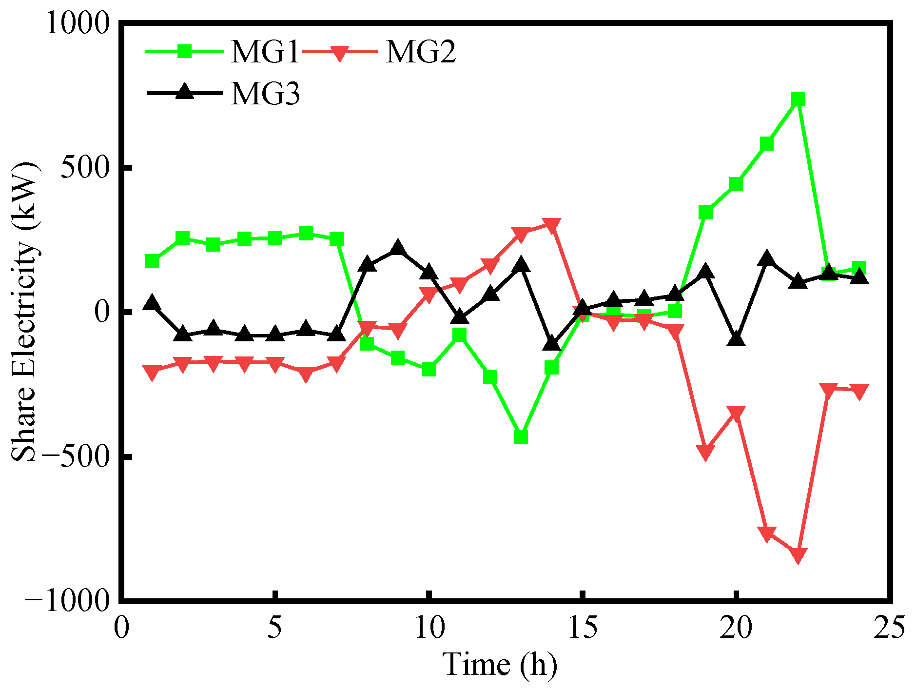
6.5. Synergistic Optimization Results of Intraday Low-Carbon Technologies and Low-Carbon Policies

Section 6.3 validated the effectiveness of the low-carbon policy of tiered carbon trading, while Section 6.4 validated the effectiveness of low-carbon technologies such as hydrogen-doped natural gas and P2G–CCS coupled operation.

In order to verify the collaborative optimization of low-carbon technologies and policies, the following scenarios were established: scenario 1, which considers hydrogen-doped natural gas and P2G–CCS coupled operation and ladder-type carbon trading without considering carbon emission constraints; and scenario 2, which comprehensively considers hydrogen-doped natural gas and P2G–CCS coupled operation, carbon trading, and carbon emission constraints.

In scenario 2, the carbon emission restriction is 5%. The intraday results of costs and carbon emissions and the output of equipment for microgrid in two scenarios are shown in

Table 7. The cost and carbon emissions of microgrids under four scenarios.

Scenario	MG	Cost (CNY)	Carbon Emissions (kg)
1	1	15,570.66	14,116.20
	2	26,946.52	15,817.61
	3	9598.95	7396.81
2	1	13,942.42	13,410.39
	2	27,385.01	15,026.72
	3	9503.18	7026.96

and

Table 8. The output of microgrid equipment in different scenarios.

Scenario	MG	Grid (kWh)	Gas Energy (m3)	Electricity of CHP Unit (kWh)	Heat of CHP Unit (kWh)	Heat of GB (kWh)	Power of CCS (kWh)	Power of P2G Unit (kWh)	Power of HP (kW)
1	1	3328.50	2195.46	1066.61	1318.27	22,892.97	7954.69	6412.61	0
	2	24,793.59	2103.59	1719.49	2149.36	16,427.22	7801.07	1654.26	0
	3	3679.05	1378.86	1417.49	1771.86	10,197.53	7803.01	1131.21	0
2	1	3891.60	2207.89	899.00	1123.75	21,570.35	7981.64	5939.68	5150.82
	2	26,281.50	1935.89	231.59	289.49	18,181.55	7855.92	1498.15	0
	3	5042.38	1312.23	797.20	996.50	10,939.39	7855.65	1038.58	99.56

.

Table 7 and Table 8 indicate that the cost in scenario 2 decreases by 1285.52 (CNY), compared to scenario 1, indicating a decrease in total operating costs of 2.46%. This is because, with the addition of carbon emission constraints, there is an increase in the purchased power from the grid, a decrease in the output of the cogeneration unit within the microgrid system, a reduction in the quantity of gas procured from external suppliers, and a decrease in carbon trading costs, due to the decrease in carbon emissions. Therefore, the increase in the cost of purchased power is less than the decrease in the cost of gas purchased and the reduction in carbon trading costs.

In scenario 2, the total carbon emissions of the multi-microgrid decrease by 1866.55 kg, indicating a decrease of 5.00% in the total carbon emissions of the multi-microgrids in scenario 2 compared to scenario 1. Because scenario 2 builds upon scenario 1 by incorporating carbon emission constraints, the limitation on carbon emissions reduces the forced output of the hydrogen-doped natural gas unit, leading to a decrease in its output. Microgrids choose to use carbon-free heat pumps or increase the output of gas boilers to compensate for the heat deficit. Moreover, they increase the power of purchased electricity to fulfill the electricity and HP requirements. Therefore, since the increase in carbon emissions from purchased electricity and the increase in output of gas boilers are less than the decrease in output of cogeneration and the decrease in carbon emissions due to the use of HP, the collaborate optimization of low-carbon technologies and policies in reducing emissions in microgrid operation are verified.

In scenario 2, the total costs of intraday stage scheduling under this strategy decrease by 5.32%, and carbon emissions decrease by 17.61% compared to the day-ahead stage, verifying the effectiveness of the strategy.

In order to deeply analyze the effect of collaborative optimization of low-carbon technologies and policies, Figure 10, Figure 11 and Figure 12 show the electricity, heat, and hydrogen power balance of the microgrid in scenario 2.

Figure 10 indicates that the electrical load is mainly provided by renewable energy units, external purchased electricity, the electric energy storage unit, and the CHP unit, among which renewable energy generation provides most of the electricity demand between the energy-consuming unit. When the output of renewable energy exceeds the demand, P2G consumes a large amount of renewable energy output to improve the utilization rate of renewable energy. The electric storage unit charges energy during off-peak electricity pricing periods (23:00–7:00) and discharges stored energy output during peak electricity pricing periods (12:00–14:00 and 19:00–22:00). MG1 and MG3 share electricity, which reduces the power of external purchased electricity for MG2 and improves the economic efficiency of the multi-microgrids operation.

Figure 11 indicates that the heat load is mainly met by hydrogen-blended GB, with the shortfall mainly supplemented by the hydrogen-doped natural gas unit and heat pumps.

Figure 12 indicates that more hydrogen is utilized during the hydrogen blending process, effectively leveraging the energy advantages of hydrogen and increasing its utilization rate. The utilization of hydrogen energy does not produce carbon emissions during combustion; therefore, the microgrid can mitigate the system’s carbon emissions by hydrogen-doped natural gas.

In conclusion, the hydrogen-doped natural gas and two-stage P2G–CCS coupled operation strategy, which considers carbon emission constraints and carbon trading, as depicted in this chapter, enhances the economic and environmental performance of multi-microgrid operation.

7. Conclusions

This article proposes a cooperative optimization scheduling strategy for multi-microgrid systems under the coupling operation of natural gas–hydrogen blending systems and P2G–CCS, considering carbon trading and carbon emission constraints. Through setting up simulation experiments, the following conclusions are drawn:

• The introduced carbon trading mechanism is validated. Compared to fixed carbon trading, carbon emissions decrease by 7.51% and total costs decrease by 8.57%. Compared to no carbon trading mechanism, carbon emissions decrease by 18.41% and total costs decrease by 10.32%. Regarding the establishment of P2G–CCS coupling and hydrogen-doped natural gas units, carbon emissions decrease by 17.23% and total costs decrease by 9.17%, compared to scenarios without low-carbon equipment, effectively reducing carbon emissions and operating costs.
• The introduced P2G–CCS coupling operation and hydrogen-doped natural gas unit models are validated. Compared to conventional models, the costs of the microgrid decrease by 1176.09 (CNY), 4337.84 (CNY), and −251.4 (CNY), respectively, with carbon emissions also decreasing by 3201.24 kg, 2767.25 kg, and 1802.57 kg, respectively, reducing the costs and carbon emissions of multi-microgrids.
• This article proposes an optimization strategy, incorporating carbon emission constraints on the above basis. Through day-ahead and intraday scheduling, the experimental results show that, compared to the day-ahead stage, the total operating costs of intraday stage scheduling under this strategy decrease by 5.32%, and carbon emissions decrease by 17.61%, verifying the effectiveness of the strategy. Compared to scenarios that do not consider carbon emission constraints, the total operating costs of intraday stage scheduling under this strategy decrease by 2.46% and carbon emissions decrease by 5.00%. Therefore, the synergistic effect of low-carbon policies and low-carbon technologies on multi-microgrid optimization scheduling can further tap into the emission reduction potential of microgrids, reducing the costs and carbon emissions of multi-microgrid systems, and providing a pathway for the low-carbon transformation of the power system.

References

1. Zhang, J.; Liu, Z. Low Carbon Economic Scheduling Model for a Park Integrated Energy System Considering Integrated Demand Response, Ladder-Type Carbon Trading and Fine Utilization of Hydrogen. Energy 2024, 290, 130311. [Google Scholar] [CrossRef]
2. Wang, R.; Wen, X.; Wang, X.; Fu, Y.; Zhang, Y. Low Carbon Optimal Operation of Integrated Energy System Based on Carbon Capture Technology, LCA Carbon Emissions and Ladder-Type Carbon Trading. Appl. Energy 2022, 311, 118664. [Google Scholar] [CrossRef]
3. Gao, L.; Fei, F.; Jia, Y.; Wen, P.; Zhao, X.; Shao, H.; Feng, T.; Huo, L. Optimal Dispatching of Integrated Agricultural Energy System Considering Ladder-Type Carbon Trading Mechanism and Demand Response. Int. J. Electr. Power Energy Syst. 2024, 156, 109693. [Google Scholar] [CrossRef]
4. Wang, L.; Shi, Z.; Dai, W.; Zhu, L.; Wang, X.; Cong, H.; Shi, T.; Liu, Q. Two-Stage Stochastic Planning for Integrated Energy Systems Accounting for Carbon Trading Price Uncertainty. Int. J. Electr. Power Energy Syst. 2022, 143, 108452. [Google Scholar] [CrossRef]
5. Liu, R.; Bao, Z.; Yu, Z.; Zhang, C. Distributed Interactive Optimization of Integrated Electricity-Heat Energy Systems Considering Hierarchical Energy-Carbon Pricing in Carbon Markets. Int. J. Electr. Power Energy Syst. 2024, 155, 109628. [Google Scholar] [CrossRef]
6. Shi, Z.; Yang, Y.; Xu, Q.; Wu, C.; Hua, K. A Low-Carbon Economic Dispatch for Integrated Energy Systems with CCUS Considering Multi-Time-Scale Allocation of Carbon Allowance. Appl. Energy 2023, 351, 121841. [Google Scholar] [CrossRef]
7. Lei, D.; Zhang, Z.; Wang, Z.; Zhang, L.; Liao, W. Long-Term, Multi-Stage Low-Carbon Planning Model of Electricity-Gas-Heat Integrated Energy System Considering Ladder-Type Carbon Trading Mechanism and CCS. Energy 2023, 280, 128113. [Google Scholar] [CrossRef]
8. Dong, W.; Lu, Z.; He, L.; Geng, L.; Guo, X.; Zhang, J. Low-Carbon Optimal Planning of an Integrated Energy Station Considering Combined Power-to-Gas and Gas-Fired Units Equipped with Carbon Capture Systems. Int. J. Electr. Power Energy Syst. 2022, 138, 107966. [Google Scholar] [CrossRef]
9. Wang, S.; Wang, S.; Zhao, Q.; Dong, S.; Li, H. Optimal Dispatch of Integrated Energy Station Considering Carbon Capture and Hydrogen Demand. Energy 2023, 269, 126981. [Google Scholar] [CrossRef]
10. Gao, J.; Meng, Q.; Liu, J.; Wang, Z. Thermoelectric Optimization of Integrated Energy System Considering Wind-Photovoltaic Uncertainty, Two-Stage Power-to-Gas and Ladder-Type Carbon Trading. Renew. Energy 2024, 221, 119806. [Google Scholar] [CrossRef]
11. Bao, H.; Sun, Y.; Zheng, S. A Collaborative Training Approach for Multi Energy Systems in Low-Carbon Parks Accounting for Response Characteristics. IET Renew. Power Gener. 2024, 18, 456–475. [Google Scholar] [CrossRef]
12. Chen, J.; Tang, Z.; Huang, Y.; Qiao, A.; Liu, J. Asymmetric Nash Bargaining-Based Cooperative Energy Trading of Multi-Park Integrated Energy System under Carbon Trading Mechanism. Electr. Power Syst. Res. 2024, 228, 110033. [Google Scholar]
13. Wang, R.; Cheng, S.; Zuo, X.; Liu, Y. Optimal Management of Multi Stakeholder Integrated Energy System Considering Dual Incentive Demand Response and Carbon Trading Mechanism. Int. J. Energy Res. 2022, 46, 6246–6263. [Google Scholar] [CrossRef]
14. Zhang, M.; Yang, J.; Yu, P.; Tinajero, G.D.A.; Guan, Y.; Yan, Q.; Zhang, X.; Guo, H. Dual-Stackelberg Game-Based Trading in Community Integrated Energy System Considering Uncertain Demand Response and Carbon Trading. Sustain. Cities Soc. 2024, 101, 105088. [Google Scholar]
15. Li, Y.; Zhang, X.; Wang, Y.; Qiao, X.; Jiao, S.; Cao, Y.; Xu, Y.; Shahidehpour, M.; Shan, Z. Carbon-Oriented Optimal Operation Strategy Based on Stackelberg Game for Multiple Integrated Energy Microgrids. Electr. Power Syst. Res. 2023, 224, 109778. [Google Scholar] [CrossRef]
16. Lyu, Z.; Lai, Y.; Yi, J.; Liu, Q. Low Carbon and Economic Dispatch of the Multi-microgrids Integrated Energy System Using CCS-P2G Integrated Flexible Operation Method. Energy Sources Part Recovery Util. Environ. Eff. 2023, 45, 3617–3638. [Google Scholar] [CrossRef]
17. Liu, Y.; Li, X.; Liu, Y. A Low-Carbon and Economic Dispatch Strategy for a Multi-microgrids Based on a Meteorological Classification to Handle the Uncertainty of Wind Power. Sensors 2023, 23, 5350. [Google Scholar] [CrossRef]
18. Chen, P.; Qian, C.; Lan, L.; Guo, M.; Wu, Q.; Ren, H.; Zhang, Y. Shared Trading Strategy of Multiple Microgrids Considering Joint Carbon and Green Certificate Mechanism. Sustainability 2023, 15, 10287. [Google Scholar] [CrossRef]
19. Wang, H.; Wang, C.; Zhao, L.; Ji, X.; Yang, C.; Wang, J. Multi-Micro-Grid Main Body Electric Heating Double-Layer Sharing Strategy Based on Nash Game. Electronics 2023, 12, 214. [Google Scholar] [CrossRef]
20. Zhong, X.; Liu, Y.; Xie, K.; Xie, S. A Local Electricity and Carbon Trading Method for Multi-Energy Microgrids Considering Cross-Chain Interaction. Sensors 2022, 22, 6935. [Google Scholar] [CrossRef]
21. Zhang, Z.; Du, J.; Fedorovich, K.S.; Li, M.; Guo, J.; Xu, Z. Optimization Strategy for Power Sharing and Low-Carbon Operation of Multi-microgrids IES Based on Asymmetric Nash Bargaining. Energy Strategy Rev. 2022, 44, 100981. [Google Scholar] [CrossRef]
22. Zhang, K.; Gao, C.; Zhang, G.; Xie, T.; Li, H. Electricity and Heat Sharing Strategy of Regional Comprehensive Energy Multi-microgrids Based on Double-Layer Game. Energy 2024, 293, 130655. [Google Scholar] [CrossRef]
23. Duan, P.; Zhao, B.; Zhang, X.; Fen, M. A Day-Ahead Optimal Operation Strategy for Integrated Energy Systems in Multi-Public Buildings Based on Cooperative Game. Energy 2023, 275, 127395. [Google Scholar] [CrossRef]
24. Xu, J.; Yi, Y. Multi-microgrids Low-Carbon Economy Operation Strategy Considering Both Source and Load Uncertainty: A Nash Bargaining Approach. Energy 2023, 263, 125712. [Google Scholar] [CrossRef]
25. Lyu, Z.; Liu, Q.; Liu, B.; Zheng, L.; Yi, J.; Lai, Y. Optimal Dispatch of Regional Integrated Energy System Group Including Power to Gas Based on Energy Hub. Energies 2022, 15, 9401. [Google Scholar] [CrossRef]
26. Hu, Q.; Zhou, Y.; Ding, H.; Qin, P.; Long, Y. Optimal Scheduling of Multi-microgrids with Power to Hydrogen Considering Federated Demand Response. Front. Energy Res. 2022, 10, 1002045. [Google Scholar] [CrossRef]
27. Cui, Y.; Deng, G.; Zeng, P.; Zhong, W.; Zhao, Y.; Liu, X. Multi-Time Scale Source-Load Dispatch Method of Power System with Wind Power Considering Low-Carbon Characteristics of Carbon Capture Power Plant. Proc. CSEE 2022, 42, 5869–5886. [Google Scholar]
28. Chen, D.; Liu, F.; Liu, S. Optimization of Virtual Power Plant Scheduling Coupling with P2G-CCS and Doped with Gas Hydrogen Based on Stepped Carbon Trading. Power Syst. Technol. 2022, 46, 2042–2054. [Google Scholar]
29. Wang, K.; Liang, Y.; Jia, R.; Wu, X.; Wang, X.; Dang, P. Two-Stage Stochastic Optimal Scheduling for Multi-microgrids Networks with Natural Gas Blending with Hydrogen and Low Carbon Incentive under Uncertain Envinronments. J. Energy Storage 2023, 72, 108319. [Google Scholar] [CrossRef]
30. Guo, R.; Ye, H.; Zhao, Y. Low Carbon Dispatch of Electricity-Gas-Thermal-Storage Integrated Energy System Based on Stepped Carbon Trading. Energy Rep. 2022, 8, 449–455. [Google Scholar] [CrossRef]
31. Wang, Y.; Wang, X.; Shao, C.; Gong, N. Distributed Energy Trading for an Integrated Energy System and Electric Vehicle Charging Stations: A Nash Bargaining Game Approach. Renew. Energy 2020, 155, 513–530. [Google Scholar] [CrossRef]
32. Du, J.; Han, X.; Wang, J. Distributed Cooperation Optimization of Multi-microgrids under Grid Tariff Uncertainty: A Nash Bargaining Game Approach with Cheating Behaviors. Int. J. Electr. Power Energy Syst. 2024, 155, 109644. [Google Scholar] [CrossRef]
Figure 1. Structure of multi-microgrids.
Energies 17 01954 g001
Figure 2. Multi-energy microgrid model construction diagram.
Energies 17 01954 g002
Figure 3. P2G–CCS coupling and hydrogen-doped natural gas subsystem structure.
Energies 17 01954 g003
Figure 4. Flowchart of the model solution.
Energies 17 01954 g004
Figure 5. Forecast of renewable energy.
Energies 17 01954 g005
Figure 6. Forecast of electricity load.
Energies 17 01954 g006
Figure 7. Forecast of heat load.
Energies 17 01954 g007
Figure 8. Multi-microgrid cost iteration and residual iteration case diagrams.
Energies 17 01954 g008
Figure 9. Interaction power between microgrids.
Energies 17 01954 g009
Figure 10. Electric power balance of each microgrid under scenario 2.
Energies 17 01954 g010
Figure 11. Heat power balance of each microgrid in scenario 2.
Energies 17 01954 g011
Figure 12. Hydrogen power balance of each microgrid in scenario 2.
Energies 17 01954 g012