


Experimental Performance Comparison of High-Glide Hydrocarbon and Synthetic Refrigerant Mixtures in a High-Temperature Heat Pump
 , , , , and
Abstract
:1. Introduction
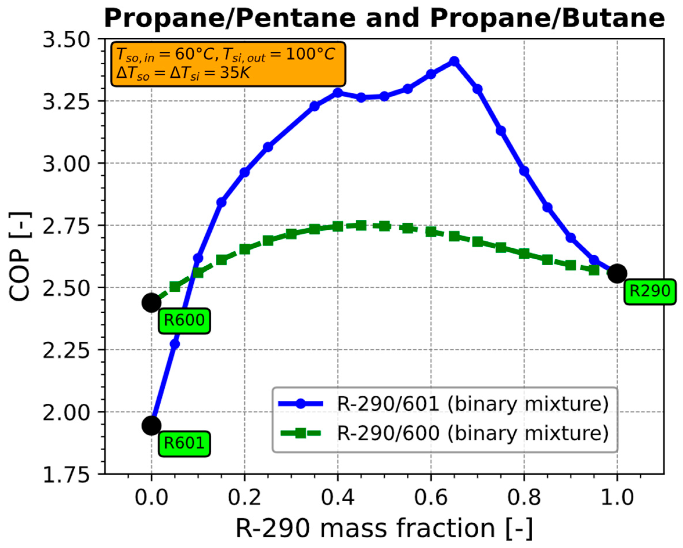
2. Modelling Results
3. Experimental Setup
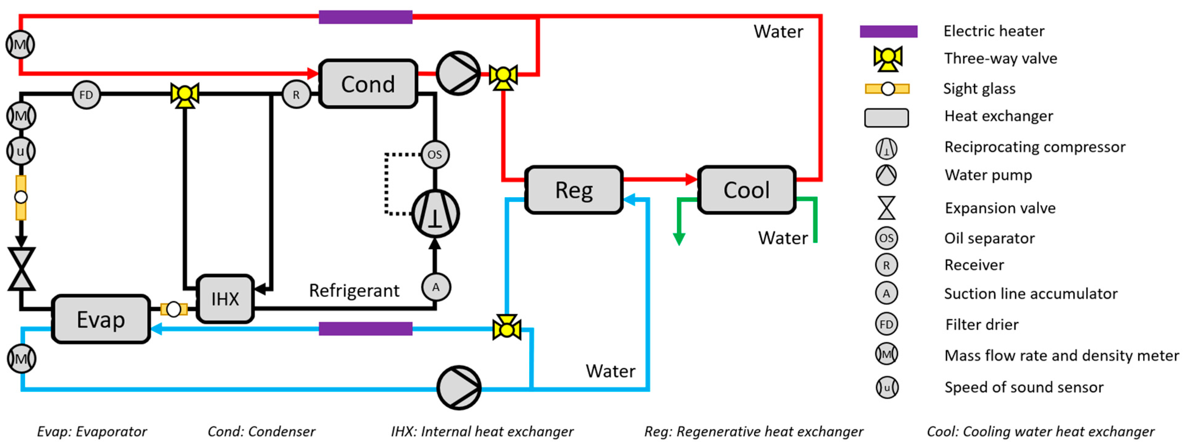
3.1. High-Temperature Heat Pump and Water Circuit Setup
- -
- Name: Reniso Triton SE 170
- -
- Type: Polyolester (POE)
- -
- Density at 15 °C: 972 kg/m3
- -
- Kinematic viscosity at 40 °C: 173 mm2/s
- -
- Kinematic viscosity at 100 °C: 17.1 mm2/s
- -
- Pourpoint: −27 °C
- -
- Flashpoint: 260 °C
- -
- Reference: [23]
- -
- Name: Reniso LPG 150
- -
- Type: Polyalkylene glycol (PAG)
- -
- Density at 15 °C: 994 kg/m3
- -
- Kinematic viscosity at 40 °C: 149.9 mm2/s
- -
- Kinematic viscosity at 100 °C: 26.2 mm2/s
- -
- Pourpoint: −42 °C
- -
- Flashpoint: 238 °C
- -
- Reference: [24]
3.2. Datasets
- Compressor A is used with synthetic refrigerants and mixtures (HFO, HCFO, and HFC).
- Compressor B is used with synthetic refrigerants and mixtures (HFO, HCFO, and HFC).
- Compressor B is used with hydrocarbon refrigerants and mixtures.
3.3. Measurement Accuracy and Steady-State Criterion
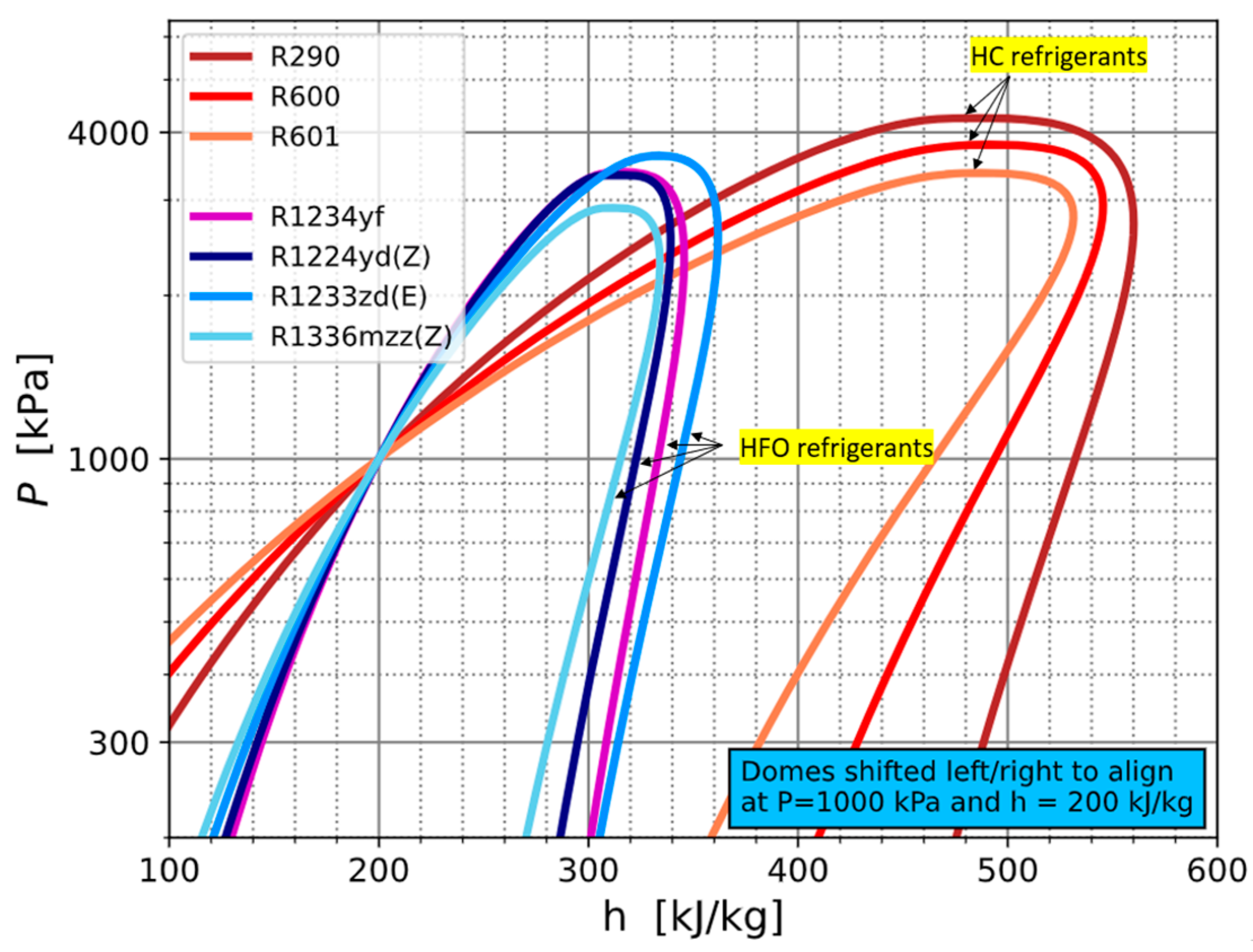
3.4. Mixture Charging Procedure and Thermophysical Properties of Refrigerants
4. Results
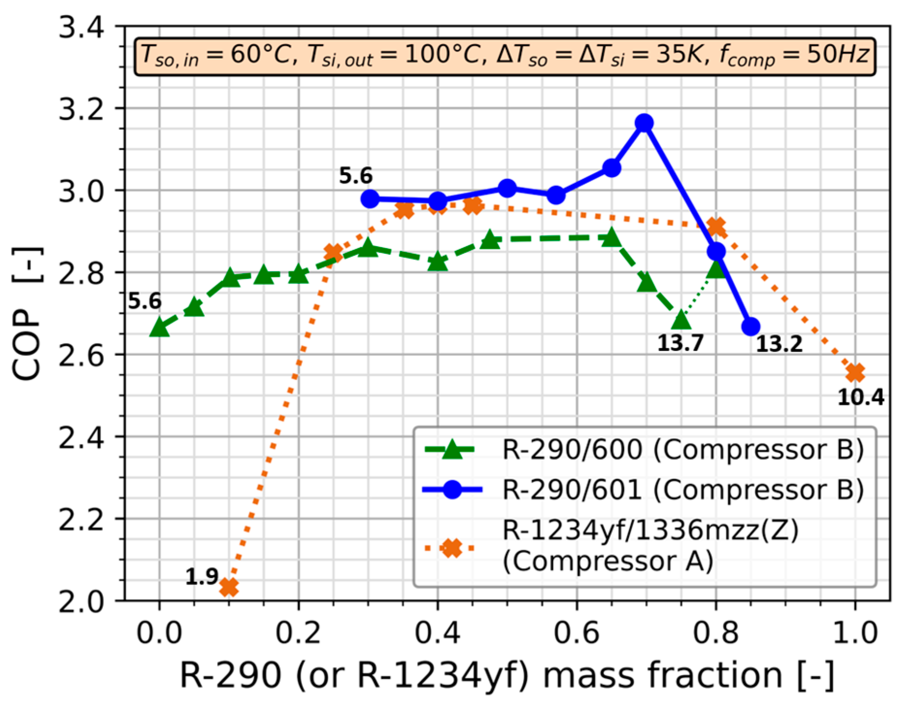
4.1. COP
4.2. Compressor Performance
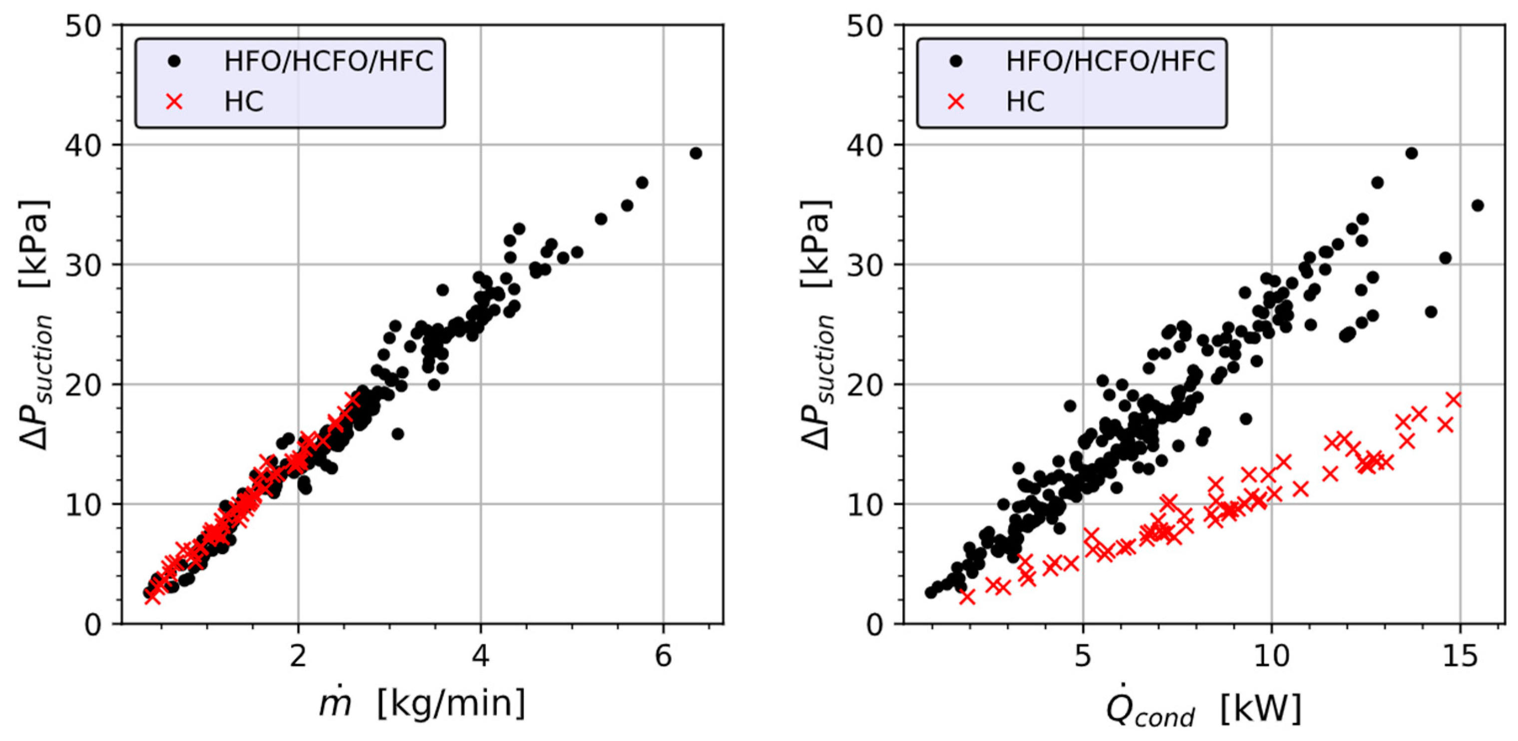
4.3. Pressure Drop
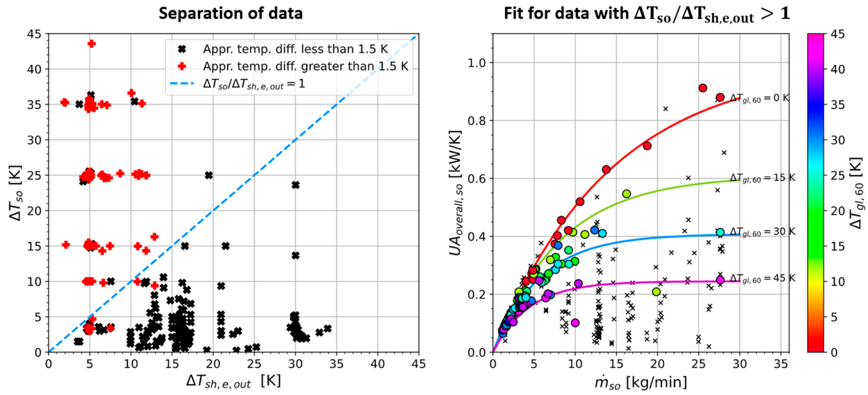
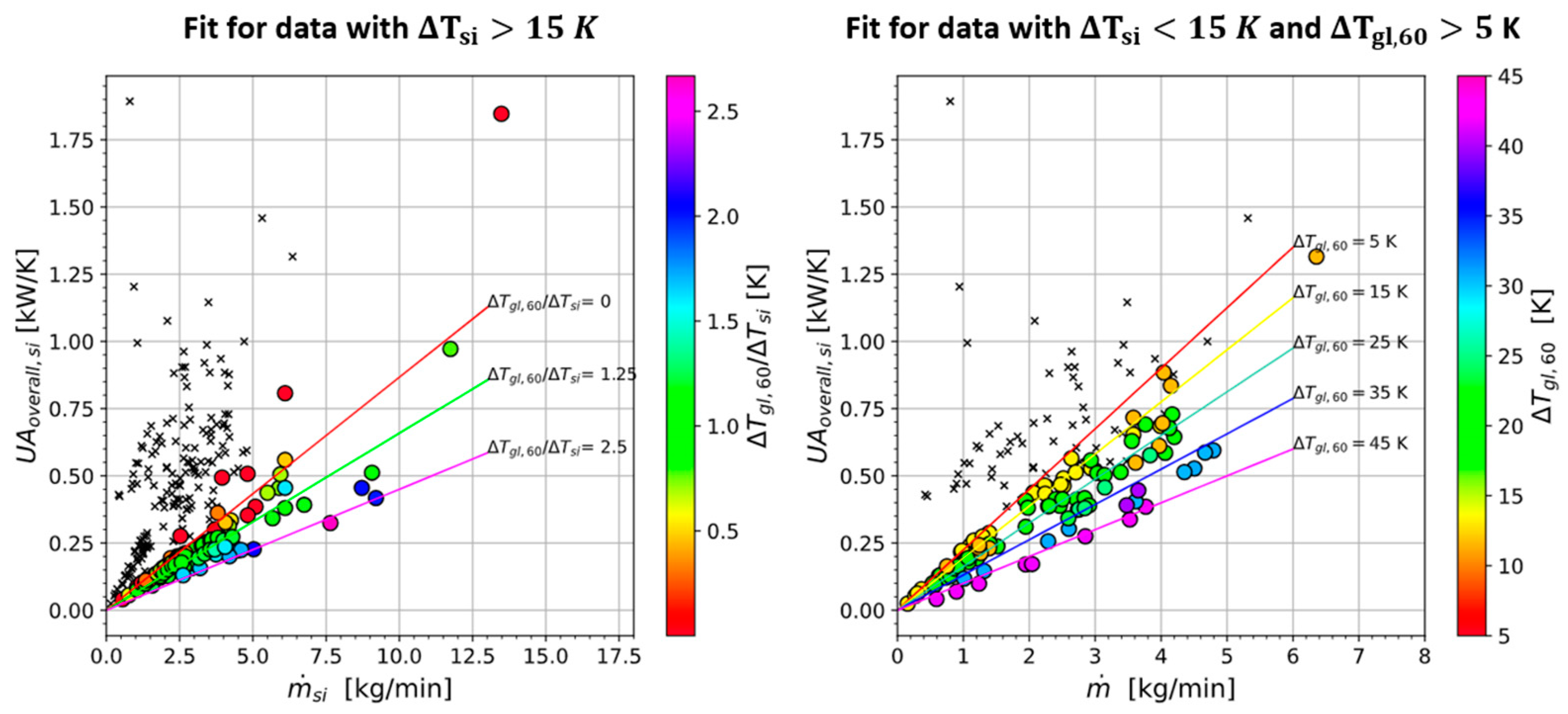
4.4. Heat Transfer
4.4.1. Introduction to Correlations
- -
- The correlations are based on more than 250 data points from four different pure fluids and 25 binary or ternary mixtures thereof with temperature glides of up to 42 K.
- -
- The operating conditions covered are very wide. For example, the evaporator outlet superheat ranged from 1.9 to 33.9 K and the evaporator inlet quality of the refrigerant ranged from 0.14 to 0.77. The heat transfer rate ranged from 0.3 to 9.8 kW, and the refrigerant inlet temperature ranged from −15 to 73 °C.
- -
- The correlations were designed using a case structure. For the evaporator and condenser, criteria for a data group were found where the ATD was below 1.5 K. The correlations predict an ATD of 1 K for all the data points meeting the criteria. Only the rest of the data is correlated with physically meaningful and specially fitted coefficients.
- -
- The correlations are based on a lumped approach to simplify their application (as opposed to a moving boundary or finite element method).
- -
- The correlations are dimensional and fitted only to one evaporator and one condenser. Unlike correlations for the heat transfer coefficient only, the presented correlations cannot be used confidently for other heat exchangers.
- -
- The evaporator was oversized for some operating conditions, which may have caused a laminar flow on the water side. Additionally, refrigerant maldistribution was detected for some operating conditions by comparing two temperature readings downstream of the evaporator at different distances.

| Dataset 1 (to Build Correlation) | Evaporator | Condenser | ||||
|---|---|---|---|---|---|---|
| Types | Flat plate heat exchangers in counterflow configuration | |||||
| Refrigerants and mixtures | Pure: R1336mzz(Z), R1233zd(E), R1224yd(Z), R1234yf Mixtures: R1336mzz(Z)/R1234yf (6), R1233zd(E)/R1234yf (3), R1224yd(Z)/R32 (5), R1224yd(Z)/R32/R1336mzz(Z) (1), R1224yd(Z)/R32/R1234yf (8), R1336mzz(Z)/R1234yf/R32 (2) * Letters (for reference with Table A2): A, B, C, D, E, F, G, H, J, K, K2, L, M, N, O, P, Q, R, S, T, V, W, X, Y, Z, AA, AB, AC, AD, AE | |||||
| Conditions to include points |
|
| ||||
| Number of data points | 274 | 266 | ||||
| Ranges of experimental data | Variable | Min | Max | Variable | Min | Max |
| 0 | 42 | 0 | 42 | |||
| 1.9 | 33.9 | 1.3 | 47.1 | |||
| 0.14 | 0.77 | ** | −6.0 | 8.0 | ||
| 0.2 | 43.6 | 0.5 | 44.9 | |||
| 0.16 | 6.88 | 0.27 | 6.88 | |||
| 0.9 | 28.1 | 0.6 | 29.0 | |||
| 48 | 984 | 208 | 3229 | |||
| *** | 0.3 | 9.8 | *** | 0.8 | 14.0 | |
| 4 | 98 | 34 | 144 | |||
| [°C] | −15 | 73 | [°C] | 60 | 158 | |
| −1.1 | 15.8 | −1.1 | 5.7 | |||
| Performance: Prediction of saturation temperature | ||||||
| 0 to 3 K | 73% | 0 to 3 K | 85% | |||
| 3 to 6 K | 25% | 3 to 6 K | 10% | |||
| 6 to 10 K | 2% | 6 to 10 K | 3% | |||
| 10 to 25 K | 0% | 10 to 25 K | 1% | |||
| 25 K or nan | 0% | 25 K or nan | 1% | |||
| Dataset 2 (to Validate Correlation) | Evaporator | Condenser | ||||
|---|---|---|---|---|---|---|
| Types | Flat plate heat exchangers in counterflow configuration | |||||
| Refrigerants and mixtures | Pure: R-1224yd(Z), R134a Mixtures: R-1234yf/1224yd(Z) (3), R-1234yf/1224yd(Z)/1336mzz(Z) (2) * Letters (for reference with Table A3): AH, AI, AJ, AK, AM, AN | |||||
| Conditions to include points |
|
| ||||
| Number of data points | 66 | 66 | ||||
| Ranges of experimental data | Variable | Min | Max | Variable | Min | Max |
| 0.1 | 16 | 0 | 16 | |||
| 0.1 | 15.8 | 0.3 | 60.5 | |||
| 0.15 | 0.60 | 0.3 | 6.6 | |||
| 2.74 | 25.2 | 4.8 | 25.1 | |||
| 1.17 | 5.60 | 1.17 | 5.60 | |||
| 1.9 | 30.9 | 2.5 | 29.0 | |||
| 165 | 806 | 909 | 2732 | |||
| ** | 2.3 | 10.4 | ** | 3.0 | 15.5 | |
| 15 | 67 | 33 | 123 | |||
| [°C] | 11.8 | 61 | [°C] | 69 | 148 | |
| −1.1 | 8.4 | −0.2 | 6.6 | |||
| Performance: Prediction of saturation temperature | ||||||
| 0 to 3 K | 92% | 0 to 3 K | 95% | |||
| 3 to 6 K | 8% | 3 to 6 K | 5% | |||
| 6 to 10 K | 0% | 6 to 10 K | 0% | |||
| 10 to 25 K | 0% | 10 to 25 K | 0% | |||
| 25 K or nan | 0% | 25 K or nan | 0% | |||
| Dataset 3 (Check Applicability to HC) | Evaporator | Condenser | ||||
|---|---|---|---|---|---|---|
| Types | Flat plate heat exchangers in counterflow configuration | |||||
| Refrigerants and mixtures | Pure: R-600 Mixtures: R-290/600 (11), R-290/601 (8) * Letters (for reference with Table A4): AO, AP, AQ, AR, AS, AT, AU, AV, AW, AX, AY, AZ, BA, BB, BC, BD, BE, BF, BG, BH, BI | |||||
| Conditions to include points |
|
| ||||
| Number of data points | 62 | 62 | ||||
| Ranges of experimental data | Variable | Min | Max | Variable | Min | Max |
| 0 | 43 | 0 | 43 | |||
| 0 | 17 | 8.3 | 52.6 | |||
| 0.08 | 0.71 | 2.0 | 14.4 | |||
| 3.7 | 35.2 | 4.8 | 35.6 | |||
| 0.40 | 2.59 | 0.40 | 2.59 | |||
| 1.8 | 30.9 | 2.08 | 26.1 | |||
| 150 | 730 | 281 | 3128 | |||
| ** | 1.1 | 11.9 | ** | 1.9 | 14.8 | |
| 14 | 56 | 28 | 124 | |||
| [°C] | −4 | 53 | [°C] | 61 | 160 | |
| −1.0 | 8.2 | 0.3 | 10.2 | |||
| Performance: Prediction of saturation temperature | ||||||
| 0 to 3 K | 82% | 0 to 3 K | 50% | |||
| 3 to 6 K | 7% | 3 to 6 K | 11% | |||
| 6 to 10 K | 11% | 6 to 10 K | 7% | |||
| 10 to 25 K | 0% | 10 to 25 K | 24% | |||
| 25 K or nan | 0% | 25 K or nan | 8% | |||
4.4.2. Evaporator Correlation
4.4.3. Condenser Correlation
4.4.4. Interpretation of Results
5. Thermophysical Properties and Composition Determination
- -
- Evaporator inlet temperature.
- -
- Dewpoint temperature
- -
- Liquid phase density
- -
- Liquid phase speed of sound
- -
- Condenser heat transfer rate
- -
- Resting pressure

6. Conclusions
Author Contributions
Funding
Data Availability Statement
Conflicts of Interest
Nomenclature
| Symbols and Abbreviations | ||
| ATD | Approach temperature difference | - |
| Coefficients in correlation | various | |
| Coefficients in correlation | various | |
| Coefficient of performance | - | |
| Difference | NA | |
| Enthalpy | kJ/kg | |
| High temperature heat pump | - | |
| Hydrofluorocarbon refrigerants | - | |
| Hydrofluoroolefin/Hydrochlorofluoroolefin refrigerants | - | |
| Hydrocarbon refrigerants | - | |
| Mass flow rate | kg/min | |
| Heat transfer rate | kW | |
| Density | kg/m3 | |
| Temperature | °C | |
| UA value | kW/K | |
| Swept volume | liter | |
| Compressor power draw | kW | |
| Vapor quality or mass fraction | - | |
| Subscripts | ||
| State point 2 (compressor outlet) | ||
| Dew point temperature of 60 °C | ||
| Calculated | ||
| Condenser | ||
| Critical temperature or pressure | ||
| Driving potential | ||
| Evaporator | ||
| Saturated liquid | ||
| Saturated vapor | ||
| Glide | ||
| Hot side | ||
| Inlet | ||
| Internal heat exchanger | ||
| Measured | ||
| Overall isentropic | ||
| Outlet | ||
| Overall | ||
| Ratio | ||
| Refrigerant | ||
| Isentropic | ||
| Suction state | ||
| Sink | ||
| Superheat | ||
| Subcooling | ||
| Source | ||
| Volumetric | ||
| Water |
Appendix A
Appendix A.1. Temperature Glide of a Mixture
Appendix A.2. Testing of Flammable Refrigerants

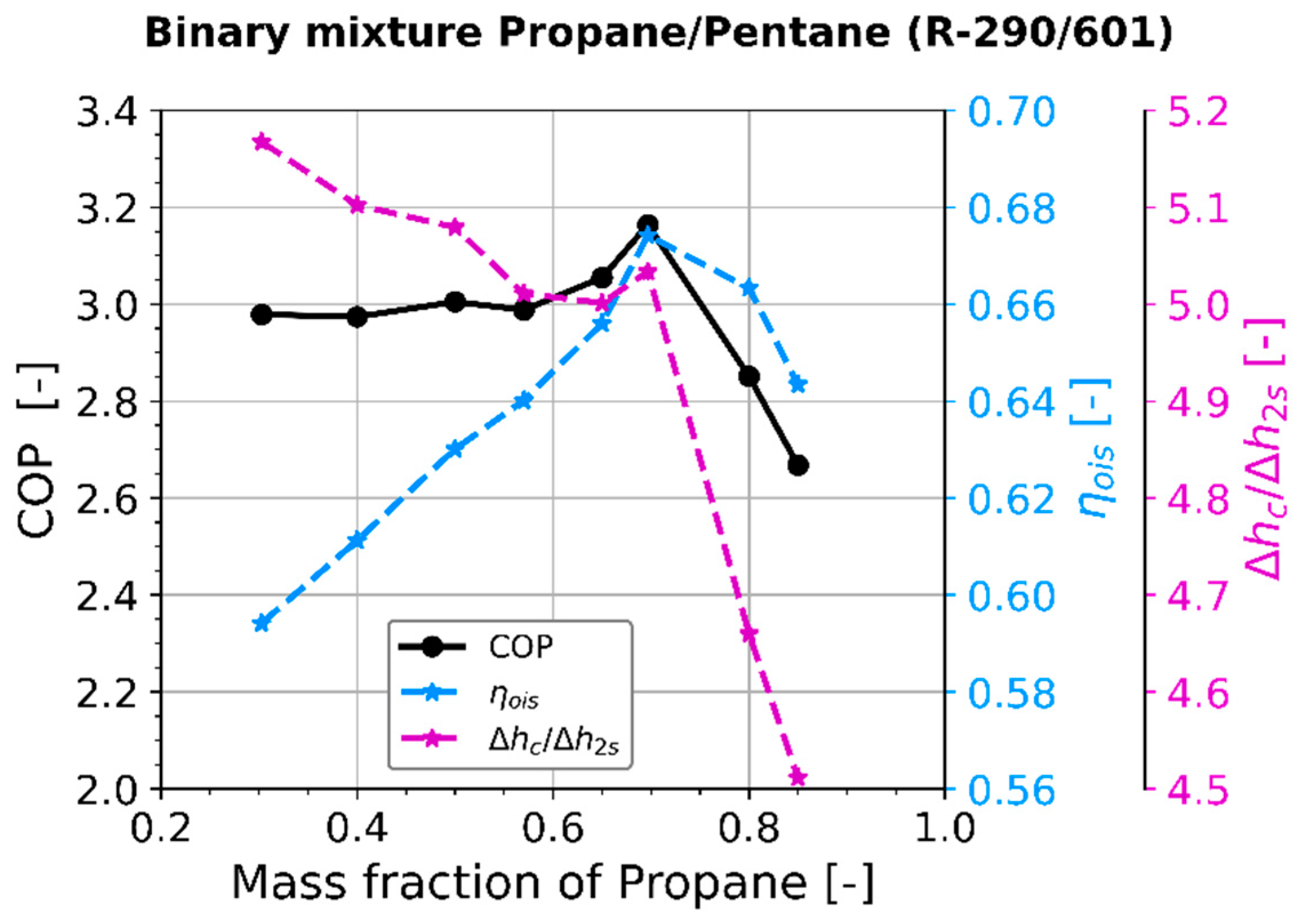
Appendix A.3. Separation of COP into Effects of Compressor and Effects of Refrigerant Properties
Appendix A.4. Single Phase Pressure Drop with a Linear Dependence on Mass Flow Rate

Appendix A.5. Methods for REFPROP Checks and Composition Determination
| Name and Functional Form | Primary Path to Reference Property | Secondary Path to Reference Property |
|---|---|---|
| Obtaining property without using REFPROP | Obtaining property using REFPROP | |
| Evaporator inlet temperature () | Direct measurement of | |
| Note: Assume isenthalpic expansion | ||
| Dewpoint temperature () | Direct measurement of | |
| Density () | Direct measurement of | |
| Speed of sound () | Direct measurement of | |
| Condenser heat transfer rate () | ||
| Note: Assume energy balance closed | ||
| Resting pressure () | Direct measurement | |
Appendix A.6. Overview of Datasets
| Letter | Type | Mixture Components | Charge and Composition | Operating Conditions | Number of Data Points | |||||||||||
|---|---|---|---|---|---|---|---|---|---|---|---|---|---|---|---|---|
| Refrigerant 1 | Refrigerant 2 | Refrigerant 3 | Charge [g] | x1 | x2 | x3 | Plow [kPa] | Phigh [kPa] | Total | with IXH | w/o IHX | DP | RP | Disc. | ||
| A | Pure | R-1233zd(E) | 4500 | 52–481 | 200–2544 | 26 | 5 | 15 | 5 | 1 | 3 | |||||
| E | Pure | R-1336mzz(Z) | 4500 | 48–357 | 315–1745 | 31 | 9 | 18 | 3 | 1 | 0 | |||||
| H | Pure | R-1234yf | 4500 | 164–984 | 1149–3168 | 23 | 7 | 13 | 2 | 1 | 8 | |||||
| K | Pure | R-1224yd(Z) | 4502 | 111–384 | 880–2389 | 21 | 9 | 8 | 3 | 1 | 0 | |||||
| K2 | Pure | R-1224yd(Z) | 4000 | 147–258 | 833–1725 | 19 | 12 | 7 | 0 | 0 | 2 | |||||
| B | Binary | R-1233zd(E) | R-1234yf | 5293 | 0.85 | 0.15 | 52–486 | 482–2609 | 38 | 8 | 25 | 4 | 1 | 8 | ||
| C | Binary | R-1233zd(E) | R-1234yf | 4500 | 0.7 | 0.3 | 104–524 | 813–2659 | 29 | 18 | 8 | 3 | 0 | 9 | ||
| D | Binary | R-1233zd(E) | R-1234yf | 5727 | 0.55 | 0.45 | 106–602 | 683–2719 | 22 | 7 | 10 | 4 | 1 | 5 | ||
| F | Binary | R-1336mzz(Z) | R-1234yf | 5000 | 0.9 | 0.1 | 77–437 | 479–2059 | 21 | 10 | 7 | 3 | 1 | 13 | ||
| G | Binary | R-1336mzz(Z) | R-1234yf | 6000 | 0.75 | 0.25 | 110–546 | 700–2037 | 16 | 11 | 2 | 3 | 0 | 10 | ||
| AA | Binary | R-1336mzz(Z) | R-1234yf | 3714 | 0.65 | 0.35 | 209–250 | 1200–1324 | 4 | 2 | 0 | 1 | 1 | 0 | ||
| AB | Binary | R-1336mzz(Z) | R-1234yf | 4010 | 0.6 | 0.4 | 228–270 | 1286–1419 | 2 | 2 | 0 | 0 | 0 | 0 | ||
| AC | Binary | R-1336mzz(Z) | R-1234yf | 4375 | 0.55 | 0.45 | 251–295 | 1398–1548 | 4 | 2 | 0 | 1 | 1 | 0 | ||
| J | Binary | R-1336mzz(Z) | R-1234yf | 6000 | 0.2 | 0.8 | 158–809 | 738–2797 | 22 | 10 | 8 | 3 | 1 | 5 | ||
| P | Binary | R-1224yd(Z) | R-32 | 4040 | 0.99 | 0.01 | 157–217 | 1057–1114 | 2 | 2 | 0 | 0 | 0 | 0 | ||
| Q | Binary | R-1224yd(Z) | R-32 | 4124 | 0.97 | 0.03 | 185–245 | 1150–1231 | 3 | 2 | 0 | 0 | 1 | 0 | ||
| L | Binary | R-1224yd(Z) | R-32 | 4739 | 0.95 | 0.05 | 213–293 | 1245–1381 | 9 | 5 | 0 | 3 | 1 | 2 | ||
| M | Binary | R-1224yd(Z) | R-32 | 5002 | 0.9 | 0.1 | 259–352 | 1628–1867 | 6 | 4 | 0 | 2 | 0 | 1 | ||
| N | Binary | R-1224yd(Z) | R-32 | 5424 | 0.83 | 0.17 | 153–584 | 1717–3122 | 14 | 7 | 4 | 2 | 1 | 5 | ||
| O | Ternary | R-1224yd(Z) | R-32 | R-1336mzz(Z) | 6029 | 0.75 | 0.15 | 0.1 | 190–536 | 1502–2980 | 8 | 5 | 0 | 2 | 1 | 1 |
| R | Ternary | R-1224yd(Z) | R-32 | R-1234yf | 4341 | 0.92 | 0.03 | 0.05 | 206–259 | 1227–1307 | 2 | 2 | 0 | 0 | 0 | 0 |
| S | Ternary | R-1224yd(Z) | R-32 | R-1234yf | 4593 | 0.87 | 0.03 | 0.1 | 223–452 | 1305–1778 | 13 | 8 | 0 | 3 | 2 | 2 |
| T | Ternary | R-1224yd(Z) | R-32 | R-1234yf | 4851 | 0.82 | 0.03 | 0.15 | 240–348 | 1361–1649 | 4 | 3 | 0 | 0 | 1 | 0 |
| V | Ternary | R-1224yd(Z) | R-32 | R-1234yf | 5155 | 0.78 | 0.02 | 0.2 | 256–308 | 1448–1566 | 2 | 2 | 0 | 0 | 0 | 0 |
| W | Ternary | R-1224yd(Z) | R-32 | R-1234yf | 5498 | 0.73 | 0.02 | 0.25 | 272–327 | 1534–2064 | 8 | 2 | 3 | 1 | 2 | 2 |
| X | Ternary | R-1224yd(Z) | R-32 | R-1234yf | 5540 | 0.72 | 0.03 | 0.25 | 278–293 | 1561–1583 | 3 | 3 | 0 | 0 | 0 | 0 |
| Y | Ternary | R-1224yd(Z) | R-32 | R-1234yf | 5599 | 0.71 | 0.04 | 0.25 | 287–295 | 1639–1661 | 4 | 2 | 0 | 1 | 1 | 0 |
| Z | Ternary | R-1224yd(Z) | R-32 | R-1234yf | 5718 | 0.7 | 0.06 | 0.24 | 312–614 | 1805–2548 | 9 | 6 | 0 | 2 | 1 | 0 |
| AD | Ternary | R-1336mzz(Z) | R-1234yf | R-32 | 4464 | 0.54 | 0.44 | 0.02 | 267–310 | 1531–1692 | 3 | 2 | 0 | 1 | 0 | 0 |
| AE | Ternary | R-1336mzz(Z) | R-1234yf | R-32 | 4605 | 0.52 | 0.43 | 0.05 | 197–591 | 1291–2655 | 12 | 7 | 0 | 3 | 2 | 0 |
| All | R-1336mzz(Z), R-1233zd(E), R-1224yd(Z), R-1234yf, R-32 and mixtures | 48–984 | 200–3168 | 380 | 174 | 128 | 55 | 23 | 76 | |||||||
| Letter | Type | Mixture Components | Charge and Composition | Operating Conditions | Number of Data Points | |||||||||||
|---|---|---|---|---|---|---|---|---|---|---|---|---|---|---|---|---|
| Refrigerant 1 | Refrigerant 2 | Refrigerant 3 | Charge [g] | x1 | x2 | x3 | Plow [kPa] | Phigh [kPa] | Total | with IHX | w/o IHX | DP | RP | Disc. | ||
| AN | Pure | R-134a | 2500 | 431–806 | 867–2689 | 23 | 19 | 4 | 0 | 0 | 0 | |||||
| AH | Pure | R-1224yd(Z) | 3503 | 207–476 | 1045–1785 | 13 | 10 | 1 | 1 | 1 | 0 | |||||
| AI | Binary | R-1224yd(Z) | R-1234yf | 3893 | 0.90 | 0.10 | 254–254 | 1216–1216 | 1 | 1 | 0 | 0 | 0 | 0 | ||
| AJ | Binary | R-1224yd(Z) | R-1234yf | 4379 | 0.80 | 0.20 | 303–303 | 1422–1422 | 1 | 1 | 0 | 0 | 0 | 0 | ||
| AK | Binary | R-1224yd(Z) | R-1234yf | 4671 | 0.75 | 0.25 | 312–528 | 1514–2447 | 13 | 10 | 2 | 1 | 0 | 0 | ||
| AM | Ternary | R-1224yd(Z) | R-1234yf | R-1336mzz(Z) | 5839 | 0.60 | 0.20 | 0.20 | 165–618 | 1292–2279 | 30 | 25 | 1 | 3 | 1 | 1 |
| All | R-134a, R-1224yd(Z), R-1234yf, R1336mzz(Z) and mixtures | 165–806 | 867–2689 | 81 | 66 | 8 | 5 | 2 | 1 | |||||||
| Letter | Type | Mixture Components | Charge and Composition | Operating Conditions | Number of Data Points | |||||||||||
|---|---|---|---|---|---|---|---|---|---|---|---|---|---|---|---|---|
| Refrigerant 1 | Refrigerant 2 | Refrigerant 3 | Charge [g] | x1 | x2 | x3 | Plow [kPa] | Phigh [kPa] | Total | with IHX | w/o IHX | DP | RP | Disc. | ||
| AP | Pure | R-600 | 1850 | 154–535 | 268–2489 | 16 | 8 | 8 | 0 | 0 | 0 | |||||
| AQ | Binary | R-600 | R-290 | 1947 | 0.95 | 0.05 | 265–265 | 1406–1406 | 1 | 1 | 0 | 0 | 0 | 0 | ||
| AR | Binary | R-600 | R-290 | 2059 | 0.90 | 0.10 | 293–293 | 1504–1504 | 1 | 1 | 0 | 0 | 0 | 0 | ||
| AS | Binary | R-600 | R-290 | 2176 | 0.85 | 0.15 | 315–323 | 1604–1628 | 2 | 2 | 0 | 0 | 0 | 0 | ||
| AT | Binary | R-600 | R-290 | 2312 | 0.80 | 0.20 | 150–683 | 416–2204 | 15 | 8 | 5 | 1 | 1 | 0 | ||
| AU | Binary | R-600 | R-290 | 2642 | 0.70 | 0.30 | 407–407 | 1951–1951 | 1 | 1 | 0 | 0 | 0 | 0 | ||
| AV | Binary | R-600 | R-290 | 3083 | 0.60 | 0.40 | 452–452 | 2156–2156 | 1 | 1 | 0 | 0 | 0 | 0 | ||
| AW | Binary | R-600 | R-290 | 3524 | 0.52 | 0.48 | 512–512 | 2332–2332 | 1 | 1 | 0 | 0 | 0 | 0 | ||
| BF | Binary | R-600 | R-290 | 1857 | 0.35 | 0.65 | 642–642 | 2622–2622 | 1 | 1 | 0 | 0 | 0 | 0 | ||
| BG | Binary | R-600 | R-290 | 2172 | 0.30 | 0.70 | 642–642 | 2721–2721 | 1 | 1 | 0 | 0 | 0 | 0 | ||
| BH | Binary | R-600 | R-290 | 2600 | 0.25 | 0.75 | 655–655 | 2828–2828 | 1 | 1 | 0 | 0 | 0 | 0 | ||
| BI | Binary | R-600 | R-290 | 3250 | 0.20 | 0.80 | 626–730 | 629–3104 | 2 | 1 | 0 | 0 | 1 | 0 | ||
| AX | Binary | R-601 | R-290 | 1587 | 0.70 | 0.30 | 232–232 | 1310–1310 | 1 | 1 | 0 | 0 | 0 | 0 | ||
| AY | Binary | R-601 | R-290 | 1845 | 0.60 | 0.40 | 304–304 | 1630–1630 | 1 | 1 | 0 | 0 | 0 | 0 | ||
| AZ | Binary | R-601 | R-290 | 2214 | 0.50 | 0.50 | 311–458 | 1654–2730 | 9 | 7 | 1 | 1 | 0 | 0 | ||
| BA | Binary | R-601 | R-290 | 2575 | 0.43 | 0.57 | 464–464 | 2162–2162 | 1 | 1 | 0 | 0 | 0 | 0 | ||
| BB | Binary | R-601 | R-290 | 3163 | 0.35 | 0.65 | 543–543 | 2342–2342 | 1 | 1 | 0 | 0 | 0 | 0 | ||
| BC | Binary | R-601 | R-290 | 2427 | 0.3 | 0.7 | 474–724 | 1331–2893 | 4 | 4 | 0 | 0 | 0 | 0 | ||
| BD | Binary | R-601 | R-290 | 2231 | 0.2 | 0.8 | 309–645 | 2069–2723 | 2 | 1 | 1 | 0 | 0 | 0 | ||
| BE | Binary | R-601 | R-290 | 2973 | 0.15 | 0.85 | 685–685 | 2967–2967 | 1 | 1 | 0 | 0 | 0 | 0 | ||
| All | R-290, R-600, R-601 and mixtures | 150–730 | 268–3104 | 63 | 44 | 15 | 2 | 2 | 0 | |||||||
Appendix A.7. Deviation of Measured and Calculated Property for Each Method

Appendix A.8. Approach Temperature Difference
Appendix A.9. Evaporator Correlation

Appendix A.10. Condenser Correlation

References
- McLinden, M.O.; Radermacher, R. Methods for comparing the performance of pure and mixed refrigerants in the vapour compression cycle. Int. J. Refrig. 1987, 10, 318–325. [Google Scholar] [CrossRef]
- Azzolin, M.; Berto, A.; Bortolin, S.; Col, D.D. Two-Phase Heat Transfer of Low GWP Ternary Mixtures. In Proceedings of the Purdue Conferences, West Lafayette, IN, USA, 24–28 May 2021. [Google Scholar]
- Cavallini, A.; Censi, G.; Del Col, D.; Doretti, L.; Longo, G.A.; Rossetto, L. Condensation of Halogenated Refrigerants Inside Smooth Tubes. HVACR Res. 2002, 8, 429–451. [Google Scholar] [CrossRef]
- Fronk, B.M.; Garimella, S. In-tube condensation of zeotropic fluid mixtures: A review. Int. J. Refrig. 2013, 36, 534–561. [Google Scholar] [CrossRef]
- Granryd, E.; Ekroth, I.; Lundquvist, P.; Melinder, A.; Palm, B.; Rohlin, P. Refrigeration Engineering; Royal Institute of Technology: Stockholm, Sweden, 2009. [Google Scholar]
- Jige, D.; Nobunaga, M.; Nogami, T.; Inoue, N. Condensation heat transfer of refrigerant mixtures of R1234yf and R32 in multiport minichannels. In Proceedings of the 26th International Congress of Refrigeration, Paris, France, 21–25 August 2023. [Google Scholar]
- Jige, D.; Nobunaga, M.; Nogami, T.; Inoue, N. Boiling heat transfer of binary and ternary mixtures in multiple rectangular microchannels. Appl. Therm. Eng. 2023, 229, 120613. [Google Scholar] [CrossRef]
- Radermacher, R.; Hwang, Y. Vapor Compression Heat Pumps with Refrigerant Mixtures, 1st ed.; CRC Press: Boca Raton, FL, USA, 2005. [Google Scholar]
- Brendel, L.P.M.; Bernal, S.N.; Widmaier, P.; Roskosch, D.; Bardow, A.; Bertsch, S.S. High-Glide Refrigerant Blends in High-Temperature Heat Pumps: Part 1—Coefficient of Performance. Int. J. Refrig. 2024; publication in progress. [Google Scholar]
- Granryd, E. Hydrocarbons as refrigerants—An overview. Int. J. Refrig. 2001, 24, 15–24. [Google Scholar] [CrossRef]
- Kim, J.H.; Cho, J.M.; Kim, M.S. Cooling performance of several CO2/propane mixtures and glide matching with secondary heat transfer fluid. Int. J. Refrig. 2008, 31, 800–806. [Google Scholar] [CrossRef]
- Mohanraj, M.; Jayaraj, S.; Muraleedharan, C.; Chandrasekar, P. Experimental investigation of R290/R600a mixture as an alternative to R134a in a domestic refrigerator. Int. J. Therm. Sci. 2009, 48, 1036–1042. [Google Scholar] [CrossRef]
- Quenel, J.; Anders, M.; Atakan, B. Propane-isobutane mixtures in heat pumps with higher temperature lift: An experimental investigation. Therm. Sci. Eng. Prog. 2023, 42, 101907. [Google Scholar] [CrossRef]
- Venzik, V.; Roskosch, D.; Atakan, B. Propan/Isobutan-Gemische als alternative Kältemittel in Kompressionskältemaschinen: Eine experimentelle Untersuchung. Forsch. Ingenieurwesen 2020, 84, 65–77. [Google Scholar] [CrossRef]
- Venzik, V.; Roskosch, D.; Atakan, B. Propene/isobutane mixtures in heat pumps: An experimental investigation. Int. J. Refrig. 2017, 76, 84–96. [Google Scholar] [CrossRef]
- Wongwises, S.; Kamboon, A.; Orachon, B. Experimental investigation of hydrocarbon mixtures to replace HFC-134a in an automotive air conditioning system. Energy Convers. Manag. 2006, 47, 1644–1659. [Google Scholar] [CrossRef]
- Wongwises, S.; Chimres, N. Experimental study of hydrocarbon mixtures to replace HFC-134a in a domestic refrigerator. Energy Convers. Manag. 2005, 46, 85–100. [Google Scholar] [CrossRef]
- Luo, J.; Yang, K.; Liu, Y.; Zhao, Z.; Chen, G.; Wang, Q. Experimental and theoretical assessments on the systematic performance of a single-stage air-source heat pump using ternary mixture in cold regions. Appl. Therm. Eng. 2023, 234, 121300. [Google Scholar] [CrossRef]
- Luo, J.; Wang, Q.; Yang, K.; Zhao, Z.; Chen, G.; Zhang, S. Performance investigation on a novel air-source heat pump using CO2/HC for recirculated water heater in cold regions. Sustain. Energy Technol. Assess. 2022, 53, 102496. [Google Scholar] [CrossRef]
- Brendel, L.P.M.; Bernal, S.N.; Arpagaus, C.; Roskosch, D.; Bardow, A.; Bertsch, S.S. Experimental investigation of high-glide refrigerant mixture R1233zd(E)/R1234yf in a high-temperature heat pump. In Proceedings of the International Congress of Refrigeration, Paris, France, 21–25 August 2023. [Google Scholar]
- Brendel, L.P.M.; Bernal, S.N.; Roskosch, D.; Arpagaus, C.; Bertsch, S.S. Compressor performance for varying compositions of high-glide mixtures R1233zd(E)/R1234yf and R1336mzz(Z)/R1234yf. In Proceedings of the 13th International Conference on Compressors and their Systems, London, UK, 11–13 September 2023. [Google Scholar] [CrossRef]
- Arpagaus, C.; Bless, F.; Uhlmann, M.; Büchel, E.; Frei, S. High temperature heat pump using HFO and HCFO refrigerants—System design, simulation, and first experimental results. In Proceedings of the Purdue Conferences, West Lafayette, IN, USA, 9–12 July 2018; Available online: https://docs.lib.purdue.edu/iracc/1875/ (accessed on 21 November 2023).
- Fuchs, “Reniso Triton SE170”, Fuchs Lubricants Germany GmbH. Available online: https://www.fuchs.com/de/en/product/product/148791-RENISO-TRITON-SE-170/ (accessed on 21 November 2023).
- Fuchs, “Reniso Triton LPG150”, Fuchs Lubricants Germany GmbH. Available online: https://www.fuchs.com/de/en/product/product/151011-RENISO-LPG-150/ (accessed on 21 November 2023).
- Brendel, L.P.M.; Bernal, S.N.; Hemprich, C.; Rowane, A.J.; Bell, I.H.; Roskosch, D.; Arpagaus, C.; Bardow, A.; Bertsch, S.S. High-Glide Refrigerant Blends in High-Temperature Heat Pumps: Part 2—Inline Composition Determination for Binary Mixtures. Int. J. Refrig. 2024; publication in progress. [Google Scholar]
- Brendel, L.P.M.; Wördemann, M.; Bernal, S.; Arpagaus, C.; Bertsch, S.S. High-glide refrigerant mixtures for HTHPs with different temperature changes on the heat sink and heat source. In Proceedings of the HTHP Symposium, Copenhagen, Denmark, 23–24 January 2024. [Google Scholar]
- Lemmon, E.W.; McLinden, M.O.; Wagner, W. Thermodynamic Properties of Propane. III. A Reference Equation of State for Temperatures from the Melting Line to 650 K and Pressures up to 1000 MPa. J. Chem. Eng. Data 2009, 54, 3141–3180. [Google Scholar] [CrossRef]
- Bücker, D.; Wagner, W. Reference Equations of State for the Thermodynamic Properties of Fluid Phase n-Butane and Isobutane. J. Phys. Chem. Ref. Data 2006, 35, 929–1019. [Google Scholar] [CrossRef]
- Thol, M.; Uhde, T.; Lemmon, E.W.; Span, R. Fundamental Equations of State for Hydrocarbons. Part I. Fluid Phase Equilibria. 2019. Available online: http://www.coolprop.org/fluid_properties/fluids/n-Pentane.html (accessed on 21 November 2023).
- Tillner-Roth, R.; Yokozeki, A. An International Standard Equation of State for Difluoromethane (R-32) for Temperatures from the Triple Point at 136.34 K to 435 K and Pressures up to 70 MPa. J. Phys. Chem. Ref. Data 1997, 26, 1273–1328. [Google Scholar] [CrossRef]
- Tillner-Roth, R.; Baehr, H.D. A International Standard Formulation for the Thermodynamic Properties of 1,1,1,2-Tetrafluoroethane (HFC-134a) for Temperatures from 170 K to 455 K and Pressures up to 70 MPa. J. Phys. Chem. Ref. Data 1994, 23, 657–729. [Google Scholar] [CrossRef]
- Lemmon, E.W.; Akasaka, R. An International Standard Formulation for 2,3,3,3-Tetrafluoroprop-1-ene (R1234yf) Covering Temperatures from the Triple Point Temperature to 410 K and Pressures Up to 100 MPa. Int. J. Thermophys. 2022, 43, 119. [Google Scholar] [CrossRef]
- Akasaka, R.; Fukushima, M.; Lemmon, E.W. A Helmholtz Energy Equation of State for cis-1-chloro-2,3,3,3-Tetrafluoropropene (R-1224yd(Z)). In Proceedings of the European Conference on Thermophysical Properties, Graz, Austria, 3–8 September 2017. [Google Scholar]
- Mondéjar, M.E.; McLinden, M.O.; Lemmon, E.W. Thermodynamic Properties of trans-1-Chloro-3,3,3-trifluoropropene (R1233zd(E)): Vapor Pressure, (p, ρ, T) Behavior, and Speed of Sound Measurements, and Equation of State. J. Chem. Eng. Data 2015, 60, 2477–2489. [Google Scholar] [CrossRef]
- McLinden, M.O.; Akasaka, R. Thermodynamic Properties of cis-1,1,1,4,4,4-Hexafluorobutene [R-1336mzz(Z)]: Vapor Pressure, (p, ρ, T) Behavior, and Speed of Sound Measurements and Equation of State. J. Chem. Eng. Data 2020, 65, 4201–4214. [Google Scholar] [CrossRef]
- Doughty, O.; Arpagaus, C.; Bertsch, S.S.; Brendel, L.P.M. Set of Performance Correlations for Reciprocating Compressor Covering Synthetic and Hydrocarbon Refrigerants. In Proceedings of the Purdue Conferences, West Lafayette, IN, USA; 2024. under review. [Google Scholar]
- Brendel, L.P.M.; Arpagaus, C.; Roskosch, D.; Bertsch, S.S. High-glide ternary mixtures in high-temperature heat pumps. In Proceedings of the DKV Tagung, Hannover, Germany, 22–24 November 2023. [Google Scholar]


| Property | Measurement Principle | Uncertainty |
|---|---|---|
| Temperature | K-type Thermocouples | +/−1.5 K absolute |
| High pressure | Piezoelectric | 75 kPa absolute |
| Low pressure | Piezoelectric | 15 kPa absolute |
| Density | Coriolis sensor | 10 kg/m3 |
| Mass flow rate (refrigerant) | <0.5% of reading | |
| Mass flow rate (heat sink) | Coriolis sensor | <0.5% of reading |
| Sound velocity | Measures time for propagation of wave between geometrically fixed speaker and receiver. | 0.01 m/s absolute |
| Measurement | Max. Allowed Change over 10 min | Average Measured Change over 10 min | ||
|---|---|---|---|---|
| Dataset 1 | Dataset 2 | Dataset 3 | ||
| Low side pressure | 5 kPa | 0.5 | 1.0 | 1.5 |
| High side pressure | 15 kPa | 1.6 | 2.6 | 4.8 |
| Subcooling at expansion valve inlet | 1.5 K | 0.1 | 0.1 | 0.1 |
| COP | 2.5% | 0.4 | 4 | 0.5 |
| Refrigerant | Type | [kPa] | [°C] | [°C] | [kJ/kg] | Reference for Thermodynamic Properties |
|---|---|---|---|---|---|---|
| R-290 (Propane) | HC | 4251 | 97 | −42 | 259 | [27] |
| R-600 (n-Butane) | HC | 3796 | 152 | −1 | 321 | [28] |
| R-601 (n-Pentane) | HC | 3368 | 197 | 36 | 337 | [29] |
| R-32 | HFC | 5782 | 78 | −51 | 175 | [30] |
| R-134a | HFC | 4059 | 101 | −26 | 155 | [31] |
| R-1234yf | HFO | 3382 | 95 | −30 | 110 | [32] |
| R-1224yd(Z) | HCFO | 3337 | 156 | 14 | 145 | [33] |
| R-1233zd(E) | HCFO | 3624 | 167 | 18 | 171 | [34] |
| R-1336mzz(Z) | HFO | 2903 | 171 | 33 | 151 | [35] |
| Coefficient | [-] | [-] | [-] | [-] | [1/kPa] | [-] |
|---|---|---|---|---|---|---|
| Value | 0.08244 | 0.72773 | 0.66981 | 0.01466 | 0.00838 | 0.00102 |
| Dataset 1 (Compressor A, Synthetic Refrigerants) | Dataset 2 (Compressor B, Synthetic Refrigerants) | Dataset 3 (Compressor B HC Refrigerants) | |
|---|---|---|---|
| Number of data points | 258 | 49 | 61 |
| Overall isentropic efficiency | Avg. dev.: 0.018 | Avg. dev.: 0.010 | Avg. dev.: 0.024 |
| Max. dev.: 0.049 | Max. dev.: 0.027 | Max. dev.: 0.103 | |
| Volumetric efficiency | Avg. dev.: 0.023 | Avg. dev.: 0.012 | Avg. dev.: 0.027 |
| Max. dev.: 0.064 | Max. dev.: 0.031 | Max. dev.: 0.079 |
Disclaimer/Publisher’s Note: The statements, opinions and data contained in all publications are solely those of the individual author(s) and contributor(s) and not of MDPI and/or the editor(s). MDPI and/or the editor(s) disclaim responsibility for any injury to people or property resulting from any ideas, methods, instructions or products referred to in the content. |
© 2024 by the authors. Licensee MDPI, Basel, Switzerland. This article is an open access article distributed under the terms and conditions of the Creative Commons Attribution (CC BY) license (https://creativecommons.org/licenses/by/4.0/).
Share and Cite
Brendel, L.P.M.; Bernal, S.N.; Arpagaus, C.; Roskosch, D.; Bardow, A.; Bertsch, S.S. Experimental Performance Comparison of High-Glide Hydrocarbon and Synthetic Refrigerant Mixtures in a High-Temperature Heat Pump. Energies 2024, 17, 1981. https://doi.org/10.3390/en17081981
Brendel LPM, Bernal SN, Arpagaus C, Roskosch D, Bardow A, Bertsch SS. Experimental Performance Comparison of High-Glide Hydrocarbon and Synthetic Refrigerant Mixtures in a High-Temperature Heat Pump. Energies. 2024; 17(8):1981. https://doi.org/10.3390/en17081981
Chicago/Turabian StyleBrendel, Leon P. M., Silvan N. Bernal, Cordin Arpagaus, Dennis Roskosch, André Bardow, and Stefan S. Bertsch. 2024. "Experimental Performance Comparison of High-Glide Hydrocarbon and Synthetic Refrigerant Mixtures in a High-Temperature Heat Pump" Energies 17, no. 8: 1981. https://doi.org/10.3390/en17081981