
Machine Fault Diagnosis through Vibration Analysis: Time Series Conversion to Grayscale and RGB Images for Recognition via Convolutional Neural Networks


Faculty of Automatic Control, Robotics and Electrical Engineering, Poznan University of Technology, 60-965 Poznań, Poland
Energies 2024, 17(9), 1998; https://doi.org/10.3390/en17091998
Submission received: 22 March 2024
/
Revised: 11 April 2024
/
Accepted: 19 April 2024
/
Published: 23 April 2024
(This article belongs to the Topic Predictive Analytics and Fault Diagnosis of Machines with Machine Learning Techniques)
Abstract
:Accurate and timely fault detection is crucial for ensuring the smooth operation and longevity of rotating machinery. This study explores the effectiveness of image-based approaches for machine fault diagnosis using data from a 6DOF IMU (Inertial Measurement Unit) sensor. Three novel methods are proposed. The IMU6DoF-Time2GrayscaleGrid-CNN method converts the time series sensor data into a single grayscale image, leveraging the efficiency of a grayscale representation and the power of convolutional neural networks (CNNs) for feature extraction. The IMU6DoF-Time2RGBbyType-CNN method utilizes RGB images. The IMU6DoF-Time2RGBbyAxis-CNN method employs an RGB image where each channel corresponds to a specific axis (X, Y, Z) of the sensor data. This axis-aligned representation potentially allows the CNN to learn the relationships between movements along different axes. The performance of all three methods is evaluated through extensive training and testing on a dataset containing various operational states (idle, normal, fault). All methods achieve high accuracy in classifying these states. While the grayscale method offers the fastest training convergence, the RGB-based methods might provide additional insights. The interpretability of the models is also explored using Grad-CAM visualizations. This research demonstrates the potential of image-based approaches with CNNs for robust and interpretable machine fault diagnosis using sensor data.
1. Introduction
Modern environments are teeming with complex electromechanical machinery, from factories to cities to homes. These systems are crucial for our way of life, but require effective maintenance to ensure their longevity and prevent unnecessary waste. Industrial machinery, in particular, presents a unique challenge due to its intricate nature. Proactive fault diagnosis strategies are essential to prevent production disruptions and equipment damage, ultimately leading to cost savings and environmental benefits. Machine fault diagnosis plays a pivotal role in ensuring the reliability and longevity of industrial machinery. Vibration analysis is a widely adopted technique for detecting faults in rotating machinery due to its sensitivity to subtle changes in a machine’s condition. In recent years, the application of deep learning techniques, particularly convolutional neural networks (CNNs), has shown promising results in automating fault diagnosis processes. The field of fault diagnosis is constantly evolving, with advancements in data sharing through the Internet of Things (IoT) and machine learning paving the way for more sophisticated solutions. This research explores the potential of image-based diagnostics using sensor data and convolutional neural networks (CNNs) for robust and interpretable fault detection in industrial machinery.
Effective fault diagnosis in electromechanical machines relies on selecting the appropriate sensors and signals. The choice depends on the specific machine and the fault characteristics it aims to detect. Common sensors are divided by the type of measurement: (a) mechanical quantities like vibration (a popular choice due to its sensitivity to faults) [1,2,3,4,5], displacement [6], torque [7,8], and angular velocity/position [9,10]; (b) electrical quantities like current [11,12] and voltage [13,14], can reveal issues related to power delivery and motor health; and (c) other signals like temperature (inner/outer) [15,16], sound [17,18,19], and even chemical analysis [20,21] can be valuable for specific fault types. Beyond traditional sensors, recent research explores image-based diagnostics using cameras [22,23,24,25] and signals converted into virtual images [12,26,27,28,29,30]. This versatility in sensor selection allows for a comprehensive approach to machine health monitoring and fault detection.
This article focuses on the utilization of vibration analysis coupled with CNNs for machine fault diagnosis. Specifically, it explores the transformation of vibration time series data into grayscale and red, green, and blue channel (RGB) images to leverage the power of image recognition algorithms. By converting time series data into image formats, it aims to exploit the multiaxis information inherent in vibration signals, which can enhance the discriminatory power of CNNs in fault detection. The use of CNNs for image recognition offers several advantages, including the ability to automatically learn hierarchical features from raw data and the robustness to variations in input signals. By training CNNs on a dataset comprising both normal and faulty vibration patterns, the model can learn to differentiate between different fault types and accurately classify unseen data. Vibration signals contain valuable information about the condition of machinery, reflecting changes in mechanical components such as bearings, gears, and shafts. Vibration analysis involves the study of these signals to identify abnormal patterns indicative of faults or anomalies. Traditional methods include Fourier transform-based techniques like Short-Time Fourier Transform (STFT) [1] and Continuous Wavelet Transform (CWT) [31], which provide insights into the frequency content of vibration signals.
The proposed methods of IMU6DoF-Time2GrayscaleGrid-CNN, IMU6DoF-Time2RGBbyType-CNN, and IMU6DoF-Time2RGBbyAxis-CNN draw inspiration from successful applications of image conversion and convolutional neural networks (CNNs) in fault diagnosis tasks. Prior research, particularly a study on six-switch and three-phase (6S3P) topology inverter faults [12], demonstrated the effectiveness of converting phase currents into RGB images for fault classification. This approach achieved superior accuracy compared to traditional machine learning methods such as decision trees, naive Bayes, support vector machines (SVMs), k-nearest neighbors (KNNs) or even simpler neural networks. In 6S3P inverter fault diagnosis research [12], each channel of the RGB image represented a different phase of the inverter current. This approach serves as a foundation for this work, but a key challenge arises when dealing with multiaxis data from a 6DOF IMU sensor. Unlike single-dimensional currents, data from multiple axes (accelerometer, gyroscope) need a well-defined conversion strategy for effective image representation. The existing literature acknowledges a gap in knowledge regarding how to optimally convert multiaxis data from IMU sensors into an image format suitable for CNN-based fault classification. Although some studies such as the one by Zia Ullah et al. [26] explore signal-to-image conversion, they often employ limited approaches. For instance, their work on Permanent Magnet Synchronous Motor (PMSM) fault diagnosis utilizes a two-channel RGB image, where blue represents one axis of the accelerometer, red represents the spectrum of the stator current, and green remains unused for a three-class classification task (a healthy, irreversible demagnetization fault, and a bearing fault). Similarly, Tingli Xie et al. [28] addressed multisensory fusion and CNNs by converting only three chosen signals into an RGB image. This approach was validated on various datasets, including one with three classes (an inner ring fault, an outer ring fault, and a normal condition). Yuqing Zhou et al. [29] investigated the diagnosis of rotating machinery using a three-channel RGB image formed by merging the permutation entropy from sensor data. This approach aimed to recognize one of five classes of tool wear (initial wear, slight wear, stable wear, serious wear, and failure). Ming Xu et al. [30] proposed a method for diagnosing bearing failure by converting the raw signals from three 1-axis accelerometers (located at the drive end, fan end, and base) into the R, G, and B channels of an RGB image. Converting high-dimensional sensor data to RGB images with only three channels can lead to information loss. Important details of the original signal might be discarded during the conversion process, potentially impacting the accuracy of the fault classification. Existing methods like those of Zia Ullah et al. [26] and Tingli Xie et al. [28] utilize two or three channels, failing to fully capture the richness of the multi-dimensional data from a 6DOF IMU sensor. This limited approach highlights the need for a more comprehensive strategy for handling multiaxis data from IMU sensors. The IMU6DoF-Time2GrayscaleGrid-CNN, IMU6DoF-Time2RGBbyType-CNN, and IMU6DoF-Time2RGBbyAxis-CNN methods address this gap by proposing a novel approach for converting 6DOF IMU data into grayscale, RGB by sensor, and RGB by axis alignment images that effectively capture the temporal characteristics of the vibration signals across all axes. This method paves the way for leveraging the power of CNNs for accurate fault classification in scenarios involving complex multidimensional sensor data. Additional improvement is needed in the presentation of the interpretability of CNNs, which is missing in the referred articles.
In this paper, a comprehensive investigation into the application of CNNs for machine fault diagnosis through vibration analysis is presented. The performance of the proposed method was evaluated on real-world datasets and compared with existing techniques to demonstrate its effectiveness in detecting and classifying machine faults. Additionally, the interpretability of the CNN model’s decision-making process is discussed, providing insights into the detected fault patterns and contributing to the overall trustworthiness of the diagnostic system. All three proposed methods (IMU6DoF-Time2GrayscaleGrid-CNN, IMU6DoF-Time2RGBbyType-CNN, and IMU6DoF-Time2RGBbyAxis-CNN) achieved high accuracy in classifying different operational states (idle, normal, fault) using sensor data converted into grayscale or RGB images. This suggests that image-based diagnostics using CNNs can be a viable approach for machine fault diagnosis. The grayscale method (IMU6DoF-Time2GrayscaleGrid-CNN) exhibited the fastest training convergence. This means it required fewer training epochs to achieve a desired level of accuracy compared to the RGB methods. The axis-aligned RGB method (IMU6DoF-Time2RGBbyAxis-CNN) might offer a more intuitive interpretation of the features learned by the CNN for fault detection. This is because each channel in the image directly corresponds to a specific axis of the sensor data. These findings highlight the potential of the use of image-based diagnostics with CNNs for machine fault diagnosis.
The manuscript is organized into distinct sections. In the Introduction, the research objectives and the importance of fault diagnosis in electromechanical systems are out-lined. The paper starts with a broader context in Section 2, discussing “Machine Fault Diagnosis through Vibration Analysis” and highlighting the use of image conversion techniques (grayscale and RGB) for analysis. Section 3 then focuses on practical implementation by introducing a “Demonstrator of Machine Fault Diagnosis”. The core of the research is presented in Section 4, “Results of Time Series Conversion…”. This section dives deeper into the different methods used: Section 4.1 details the IMU6DoF-Time2GrayscaleGrid-CNN method, explaining its approach. Section 4.2 and Section 4.3 follow the same structure, presenting the IMU6DoF-Time2RGBbyType-CNN method and the IMU6DoF-Time2RGBbyAxis-CNN method, respectively, with a focus on their specific functionalities. Section 5 provides a discussion of the findings, comparing the different methods and their effectiveness. Finally, Section 6 offers conclusions summarizing the key takeaways and potential future directions of the research.
2. Machine Fault Diagnosis through Vibration Analysis with Time Series Conversion to Greyscale and RGB Images
Machine fault diagnosis is a critical aspect of predictive maintenance in various industries. Vibration analysis has emerged as a prominent technique for detecting and diagnosing faults in rotating machinery due to its sensitivity to changes in machine conditions. Traditional methods often rely on a time-frequency analysis of vibration signals, requiring expert knowledge for the accurate selection of window length and window shape. In response to these challenges, in this section was proposed a novel approach for machine fault diagnosis using vibration analysis, coupled with time series conversion to greyscale and RGB images. Time series data from sensors such as Inertial Measurement Units (IMUs) play a crucial role in capturing the dynamics of machinery. By converting time series data from IMUs, specifically six-degrees-of-freedom (6DOF) sensors, into a spatial format, it enables the application of image processing methods for feature extraction and analysis. The goal is to transform the temporal information contained in the time series into a spatial representation that can be effectively analyzed using image processing techniques. By leveraging image recognition techniques, particularly convolutional neural networks (CNNs), this method aims to enhance fault detection accuracy while providing interpretable insights into fault patterns.
IMUs provide measurements of acceleration and angular velocity along three orthogonal axes, resulting in six channels of time series data. The proposed methods were verified at the fan demonstrator described in the next section. Each frame of data consists of 256 samples, with a one-sample overlap between consecutive frames. The high-resolution nature of IMU data allows for the detailed capture of machine vibrations and movements. The 16-by-16 sub-images (256 samples) are arranged in a grid pattern to form a larger greyscale image with dimensions of 48 by 32 pixels. Each pixel in the greyscale image corresponds to a specific sample in the original time series data, capturing the temporal evolution of machine behavior. Figure 1 depicts a method for recognizing a grayscale image using data from a 6DoF IMU sensor. The method, called IMU6DoF-Time2GrayscaleGrid-CNN, converts time series data into a grayscale image for recognition by a convolutional neural network (CNN). The procedure consists of these steps:
- The system collects data from the gyroscope and accelerometer of the 6DoF IMU sensor. Both sensors provide data in the time domain.
- The time series data for each axis (X, Y, and Z) is divided into segments with 256 samples each. These segments are then reshaped into 16 × 16 matrices.
- The reshaped 16 × 16 matrices from each axis (X, Y, and Z) are then combined to form a single grayscale image of a 48 × 32 size.
- The grayscale image is fed into a convolutional neural network for classification. The CNN architecture consists of convolutional layers, batch normalization, ReLU activation, fully connected layers, and a softmax layer for classification.
Overall, the IMU6DoF-Time2GrayscaleGrid-CNN method transforms time series data from a 6DoF IMU sensor into a suitable format for recognition by a CNN.
Grayscale images provide a compact and efficient way to represent the temporal evolution of sensor data. This allows for faster processing and potentially lower computational demands compared to more complex representations. The proposed IMU6DoF-Time2GrayscaleGrid-CNN method demonstrates a promising approach for machine fault diagnosis by leveraging the strengths of both vibration analysis and image recognition techniques. By converting vibration time series data into grayscale images, it allows CNNs to effectively learn features and classify faults in rotating machinery. This chapter outlines the theoretical foundation and practical implementation of this method, paving the way for further research in predictive maintenance and industrial fault diagnosis.
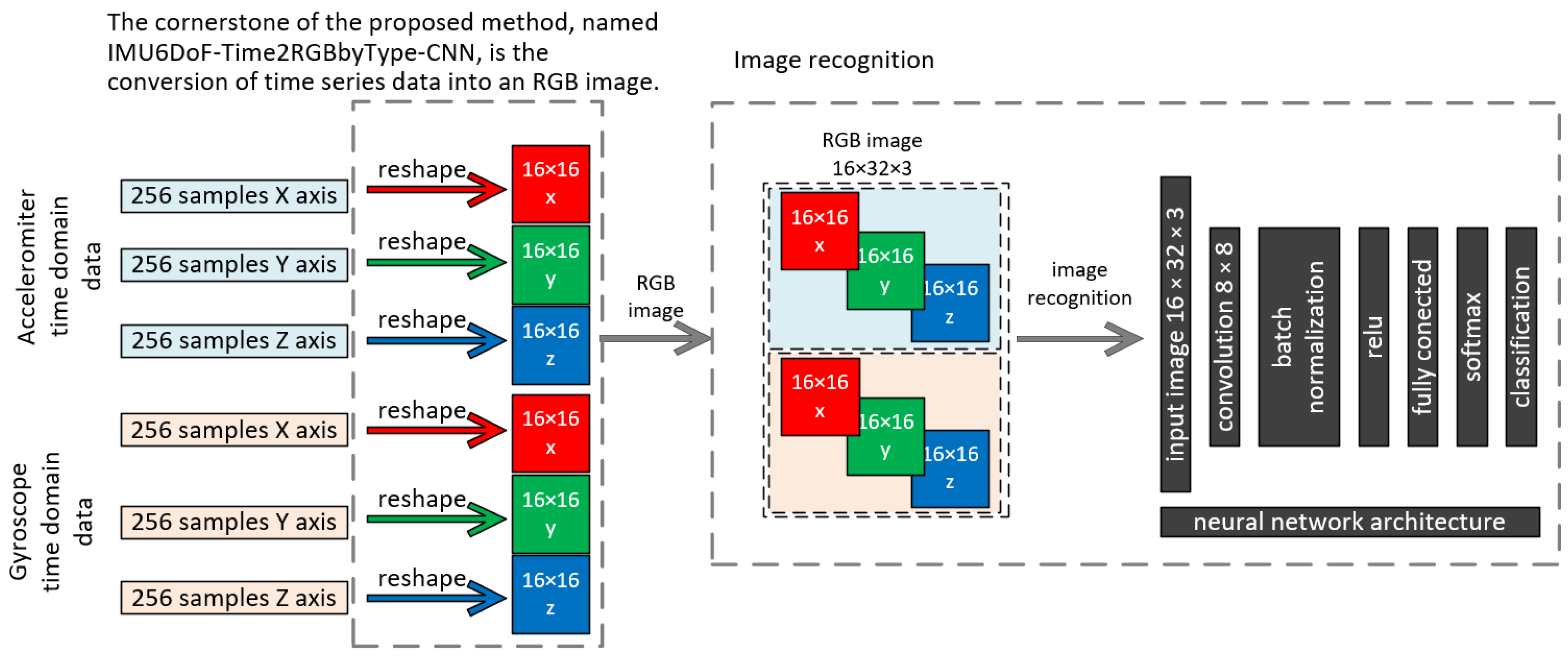
Figure 2 shows the method named IMU6DoF-Time2RGBbyType-CNN for converting time series data into an RGB image for image recognition. The method involves the following steps:
- Acquire time series data of 256 × 6 samples from the IMU 6DoF sensor.
- Reshape the time series data into a 2D image. For instance, a 256-sample time series would be reshaped into a 16 × 16 image.
- Three separate 2D images are then concatenated along the color channel to form a single RGB image. In this way, each channel of the RGB image represents the data from a single axis (X, Y, and Z) of the IMU sensor.
- The resulting RGB image can then be used for image recognition tasks using a convolutional neural network (CNN). The architecture of the CNN is shown in Figure 2, and consists of a convolutional layer, batch normalization, an ReLU layer, a fully connected layer, a soft max layer, and a classification layer.
Figure 3 depicts a method named IMU6DoF-Time2RGBbyAxis-CNN for recognizing images using data from a 6DoF IMU sensor. This method converts time series data into RGB images for recognition by a convolutional neural network (CNN). A breakdown of the process is illustrated in Figure 3:
- Data Acquisition. The system collects data from the gyroscope and accelerometer of the 6DoF IMU sensor. Both provide data in the time domain.
- Data Preprocessing. The time series data for each axis (X, Y, and Z) is segmented into 256 samples each. These segments are then reshaped into 16 × 16 matrices.
- RGB Image Formation. The reshaped 16 × 16 matrices from each axis (X, Y, and Z) are stacked together to form a single RGB image of a 48 × 16 × 3 size.
- Image Recognition using CNN. The RGB image is fed into a convolutional neural network for classification. The specific CNN architecture is provided in Figure 3; it consists of convolutional layers, batch normalization, ReLU activation, fully connected layers, and a softmax layer for classification.
Overall, the IMU6DoF-Time2RGBbyAxis-CNN method transforms time series data from a 6DoF IMU sensor into a format suitable for recognition by a CNN.
3. Demonstrator of Machine Fault Diagnosis
This section focuses on demonstrating the feasibility of the proposed methods, IMU6DoF-Time2GrayscaleGrid-CNN, IMU6DoF-Time2RGBbyType-CNN, and IMU6DoF-Time2RGBbyAxis-CNN, for image-based recognition using IMU data. A dedicated demonstrator, depicted in Figure 4, was constructed to verify their effectiveness. This proof-of-concept setup consisted of the following components: microcontroller STM32F746ZG at a NUCLEO board is responsible for collecting data from the IMU sensor and transmitting it in a JSON (JavaScript Object Notation) format via the MQTT (Message Queuing Telemetry Transport) protocol to the computational unit; a MPU6050 sensor which is a 6DoF IMU sensor that captures motion data along the X, Y, and Z axes; a computer fan acts as the target for vibration investigation; and a blue paper clip is attached to the fan blade to create an imbalance, thereby inducing controlled vibrations during operation.
The demonstrator mimics a real-world scenario where an IMU sensor can be mounted on a machine to capture vibration data for fault diagnosis. The controlled vibrations generated by the imbalanced fan blade simulate potential machine faults that the proposed methods can learn to identify. This experimental setup provides a practical validation platform to assess the performance of the proposed CNN-based approaches for image recognition from IMU data.
The proof of concept was verified in the demonstration with the Yate Loon Electronics (Taiwan) fan model GP-D12SH-12(F) DC 12 V 0.3 A. Nominal velocity was 3000 RPM (revolutions per minute), which is equivalent to 50 revolutions per second. The fan was supplied with 5 V, which is related to around 21 revolutions per second. This highlights the method’s potential to handle a range of operating conditions. The proposed method was investigated for constant rotational speed applications, which are prevalent in many industrial settings. Example applications include centrifugal pumps and blowers, machine tool spindles, conveyor belts, cooling fans in electronics, and duct fans in air conditioning. Furthermore, the potential extends beyond applications with strictly constant speeds. With its ability to handle variations in operating conditions, the IMU6DoF-Time2GrayscaleGrid-CNN, IMU6DoF-Time2RGBbyType-CNN, and IMU6DoF-Time2RGBbyAxis-CNN approaches could be applicable to scenarios with controlled speed changes or slight fluctuations, allowing their use in a wider range of industrial machinery.
IMU data was continuously acquired at a constant sampling rate of 200 Hz, corresponding to a sampling interval of 5 milliseconds (ms). This resulted in a buffer containing 256 samples, representing a total acquisition time of 1.28 s. In other words, it took 1.28 s to collect the 256 data points from the six-degrees-of-freedom (DOF) IMU sensor. The collected measurement data is sent from the microcontroller client to an MQTT broker on the laptop using the MQTT protocol. This communication flow is depicted in Figure 5.
Aliasing can be a significant concern when dealing with vibration data analysis. The key is the presence of built-in digital low-pass filters (DLPFs) within the MPU-6050 sensor. These filters play a crucial role in mitigating aliasing by attenuating high-frequency components beyond the sensor’s Nyquist rate (half the sampling rate). The configurable bandwidth settings (260 Hz, 184 Hz, 94 Hz, 44 Hz, etc.) in the sensor allows us to adjust the DLPF cutoff frequency to suit the specific requirements of the application. The vibration frequency range of interest was carefully considered for fan blade imbalance detection. To ensure that the relevant vibration components were adequately captured without aliasing, the sampling rate was selected as at least twice the highest frequency of interest. The built-in DLPFs of the MPU-6050 were used to attenuate high-frequency noise beyond the desired bandwidth.
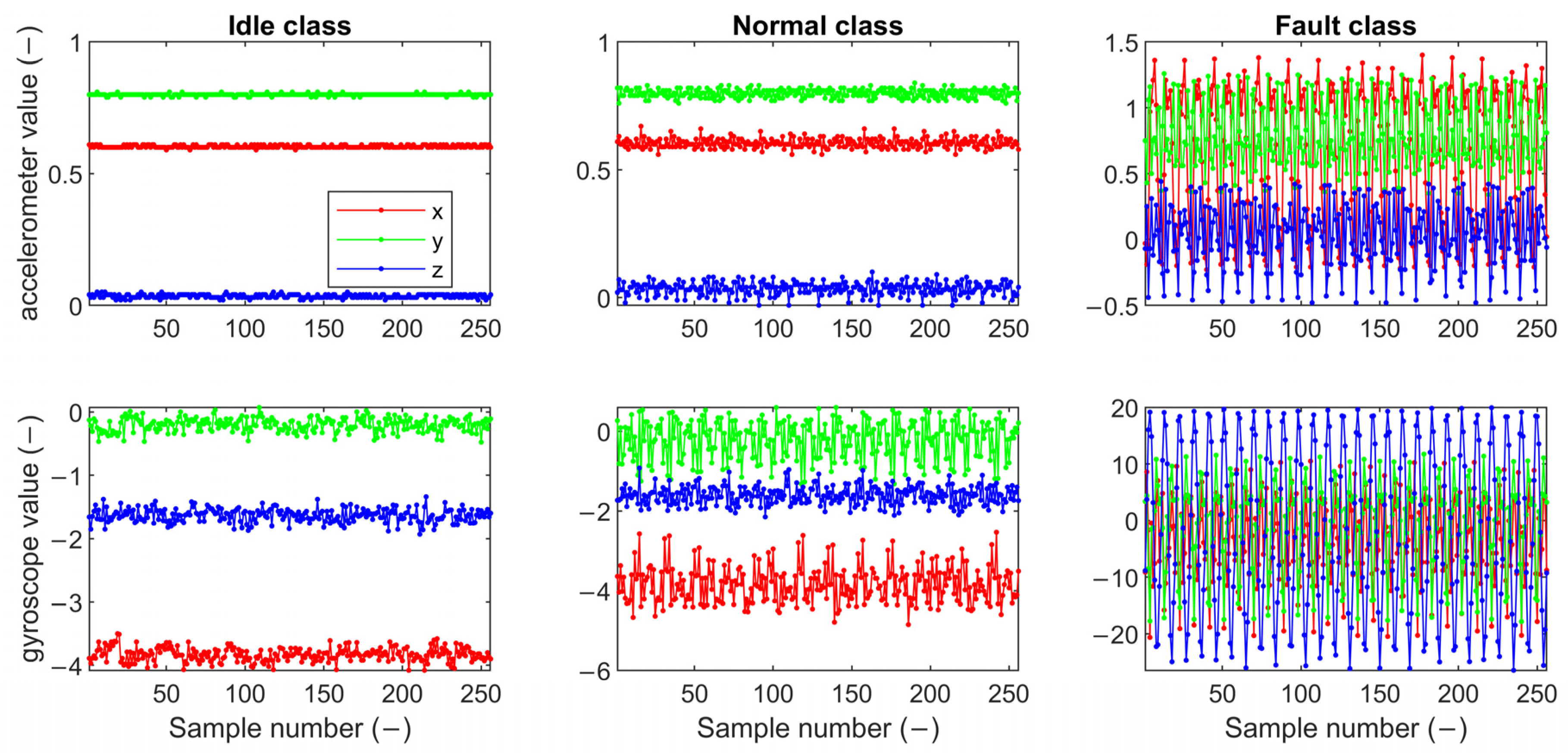
To evaluate the effectiveness of the proposed methods, data were collected for three distinct operational classes: idle, normal operation, and fault. In the fault class, a paperclip was attached to the fan blade to induce an imbalance and generate controlled vibrations, simulating a potential machine fault scenario. Time series data for each class are presented in Figure 6. Each segment of 256 IMU samples captured time series data for each of the three axes (X, Y, and Z) of the accelerometer and gyroscope, resulting in a total of six data streams per segment (256 × 6).
For each captured segment containing 256 time series samples from the three accelerometer axes (X, Y, and Z) and the three gyroscope axes (X, Y, and Z), a separate frequency domain representation was obtained using a technique like Fast Fourier Transform (FFT). This transformation converts the time-based signal from each axis into its constituent frequency components, allowing for an analysis of the dominant frequencies present in the data. The single-segment time series data converted into frequency domains for three axes of the accelerometer and gyroscope for each class are shown in Figure 7. The idle class exhibits a dominant peak at 0 Hz, signifying the absence of significant vibration. Normal operation is characterized by the presence of small vibrations spread across a frequency range of 20 Hz to 90 Hz, potentially due to motor operation or environmental factors. In contrast, the fault condition is distinguished by a dominant frequency of 20 Hz appearing specifically in the X-axis of the accelerometer data and the Z-axis of the gyroscope data. This targeted presence of a specific frequency suggests a characteristic signature induced by the imbalanced fan blade attached in the fault scenario.
4. Results of the Time Series’ Conversion to Greyscale and RGB Images and Recognition via Convolutional Neural Networks
CNNs are powerful tools for image recognition. This section evaluates three proposed methods for image-based recognition using data from a 6DoF IMU sensor: IMU6DoF-Time2GrayscaleGrid-CNN, IMU6DoF-Time2RGBbyType-CNN, and IMU6DoF-Time2RGBbyAxis-CNN. The methods were described in Section 2. Each subsection presents a representative input image for each class (idle, normal operation, and fault) to illustrate the processed data used by the corresponding CNN model. Additionally, the training progress of the CNN, visualized as a curve depicting loss or accuracy over training epochs, is provided to demonstrate the learning behavior of the model. Furthermore, confusion matrices for both the test and validation datasets are included to assess the classification performance of each method. Finally, to gain insights into the decision-making process of the CNNs, an interpretability analysis using techniques like Grad-CAM, occlusion sensitivity, and LIME is presented in each subsection.
For each method, a total of 7680 images were generated, with each class (idle, normal operation, and fault) equally represented by 2560 images. These images were then split into training and test sets using an 80/20 ratio. This means 80% (2048 images per class) were used to train the CNN models, while the remaining 20% (512 images per class) were used for testing and evaluating their performance.
4.1. The IMU6DoF-Time2GrayscaleGrid-CNN Method
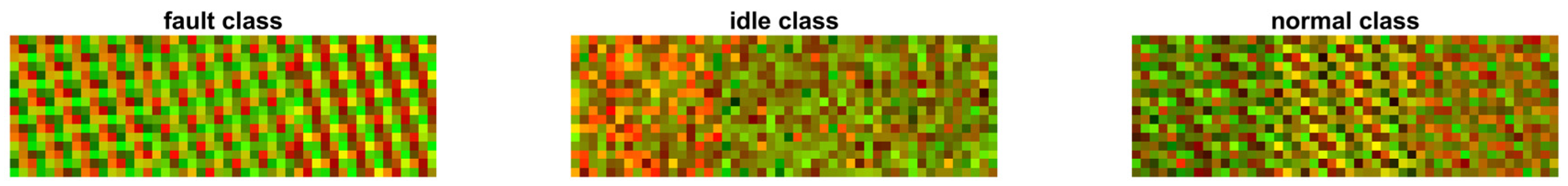
This method transforms the time series data from each axis (X, Y, and Z) into a 16 × 16 grid of grayscale values. These grids are then stacked to form a single grayscale image for classification by a CNN. For the IMU6DoF-Time2GrayscaleGrid-CNN method, representative grayscale images are presented for each class (idle, normal operation, and fault) in Figure 8. These grayscale images visually depict how the time series data from the 6DoF IMU sensor are transformed into a format suitable for classification by the CNN. The images provide insights into the patterns and variations observed in the data across different operational states.
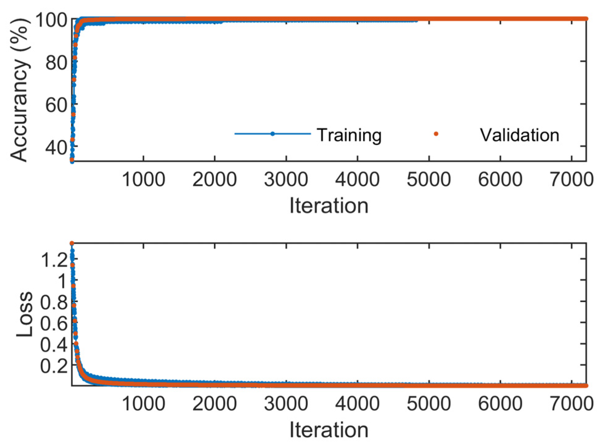
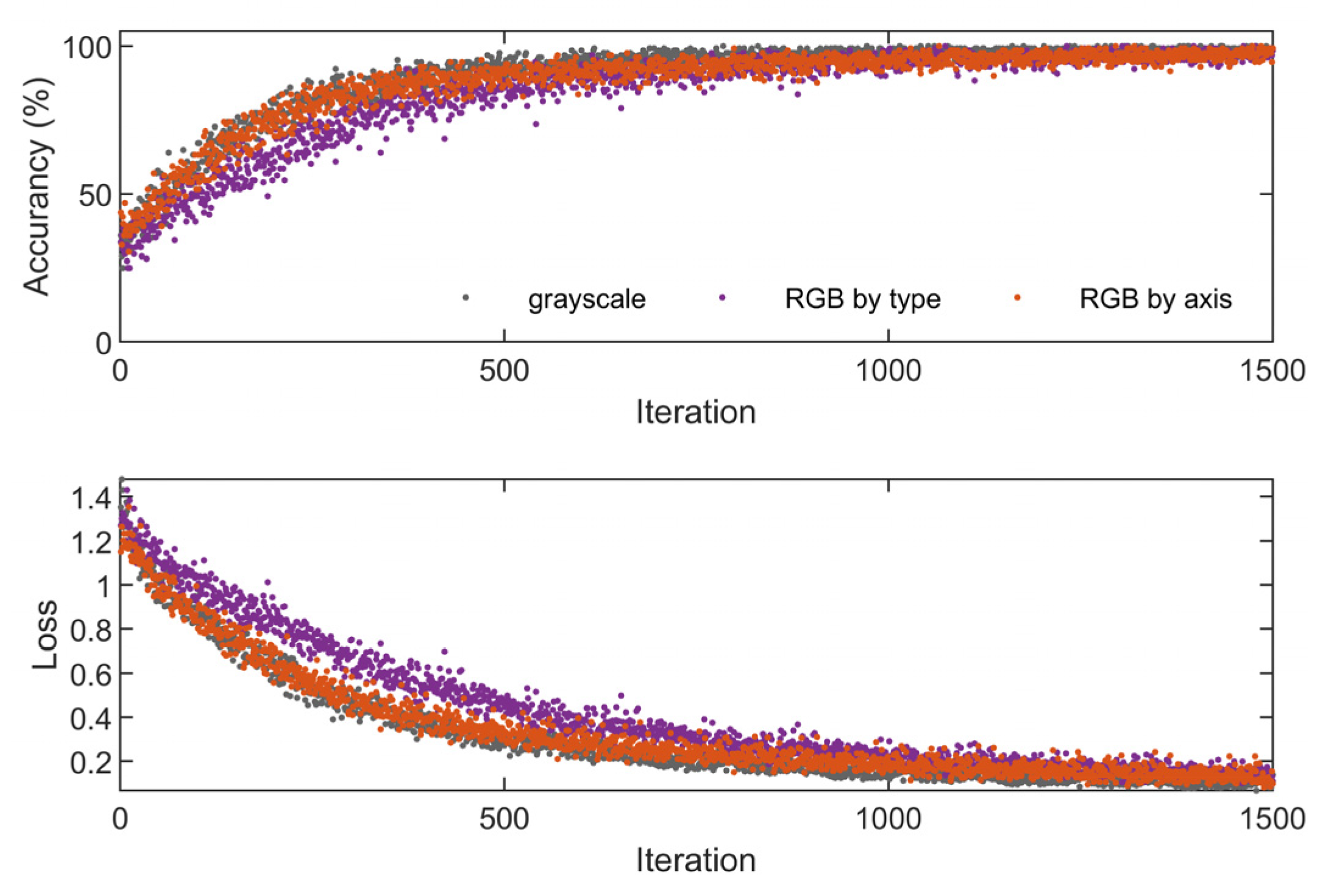
Figure 9 depicts the training progress of the convolutional neural network (CNN) used in the IMU6DoF-Time2GrayscaleGrid-CNN method. The training lasted for 150 epochs, which corresponds to a total of 7200 iterations. The learning rate was set to 0.001. The graph shows two subplots, one representing the training loss and the other representing the training accuracy. Ideally, the training loss should decrease over time as the CNN learns to improve its performance on the training data. Conversely, the training accuracy should increase as the model becomes better at correctly classifying the images. By analyzing this graph, how effectively the CNN model was trained can be assessed. A good training curve would show a steady decrease in loss and a corresponding increase in accuracy over the course of the training epochs.
Figure 10 depicts a confusion matrix, which is a table that visualizes the performance of a classification model on a test dataset. In this case, the confusion matrix shows the results of a CNN model trained to classify images generated using the IMU6DoF-Time2GrayscaleGrid-CNN method. The left side of the matrix represents the actual class labels for the test images (ground truth), while the bottom side represents the classes predicted by the CNN model. Each row of the matrix corresponds to a true class (idle, normal, fault), and each column represents a predicted class. The ideal scenario is to have high values along the diagonal of the matrix, indicating that the model correctly classified most of the images. Conversely, high values off the diagonal indicate classification errors. By analyzing the distribution of values in the confusion matrix, you can gain insights into the strengths and weaknesses of the CNN model. For instance, a high value in the top-left corner (a fault class predicted as a fault) suggests good performance in identifying fault images. However, a high value in the middle-right place (an idle class predicted as normal) would indicate that the model sometimes confuses idle images with normal operation images.
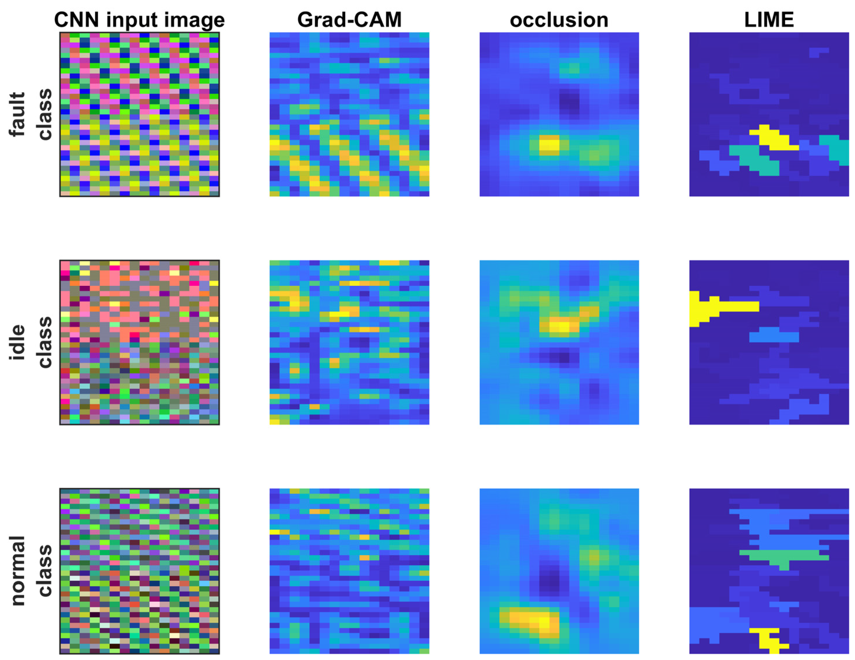
Figure 11 showcases the interpretability analysis of the IMU6DoF-Time2GrayscaleGrid-CNN method using various techniques. Each row corresponds to a class (fault, idle, normal), and the columns present different methods for gaining insights into the CNN’s decision-making process. The CNN input image column displays the grayscale image generated from the IMU data for each class. These images serve as the input to the CNN for classification. The Grad-CAM column likely shows the Grad-CAM visualizations for each class. The Grad-CAM highlights the regions in the grayscale image that the CNN focuses on when making its classification decision. By analyzing these visualizations, we can understand which parts of the image are most influential for the CNN’s prediction. For example, in the fault class, the Grad-CAM highlights specific areas corresponding to axis X of the accelerometer (top-left corner of the image) and axis Z of the gyroscope (bottom-right corner of the image) that correspond to the vibrations induced by the imbalanced fan blade. The fault condition is distinguished by a dominant frequency of 20 Hz appearing specifically in the X-axis of the accelerometer’s data and the Z-axis of the gyroscope’s data, as shown in Figure 7. The occlusion sensitivity column depicts the results of the occlusion sensitivity analysis. In this technique, different parts of the input image are systematically masked or occluded, and the impact on the CNN’s prediction is observed. If occluding a particular region significantly alters the prediction, it suggests that the CNN relied heavily on that region for classification. By analyzing the occlusion sensitivity maps, insights can be gained into which parts of the image are most informative for the CNN. The occlusion sensitivity analysis in Figure 11 complements the information gleaned from Grad-CAM visualizations. While the Grad-CAM highlights the areas of the grayscale image that receive high activation from the CNN, occlusion sensitivity takes a more direct approach. Occlusion sensitivity maps reinforce these findings. By progressively occluding these highlighted regions and observing the changes in the CNN’s predictions for the fault class, the analysis confirms their critical role. If occluding these specific areas significantly reduces the model’s confidence in classifying an image as a “fault”, it demonstrates that the CNN heavily relies on information from those regions to make that classification. In essence, while the Grad-CAM points out the areas of interest, occlusion sensitivity quantifies their importance in the CNN’s decision-making process. This combined analysis provides a more comprehensive understanding of how the CNN leverages the grayscale image data to identify fault conditions. The LIME column shows the LIME explanations for each class. LIME generates a localized explanation for a single image prediction by introducing interpretable features around the instance of interest. Here, these features might be related to specific patterns or statistical properties within the grayscale image that influence the CNN’s decision. Analyzing LIME explanations can be useful for understanding the reasoning behind the CNN’s prediction for a particular image.
4.2. The IMU6DoF-Time2RGBbyType-CNN Method
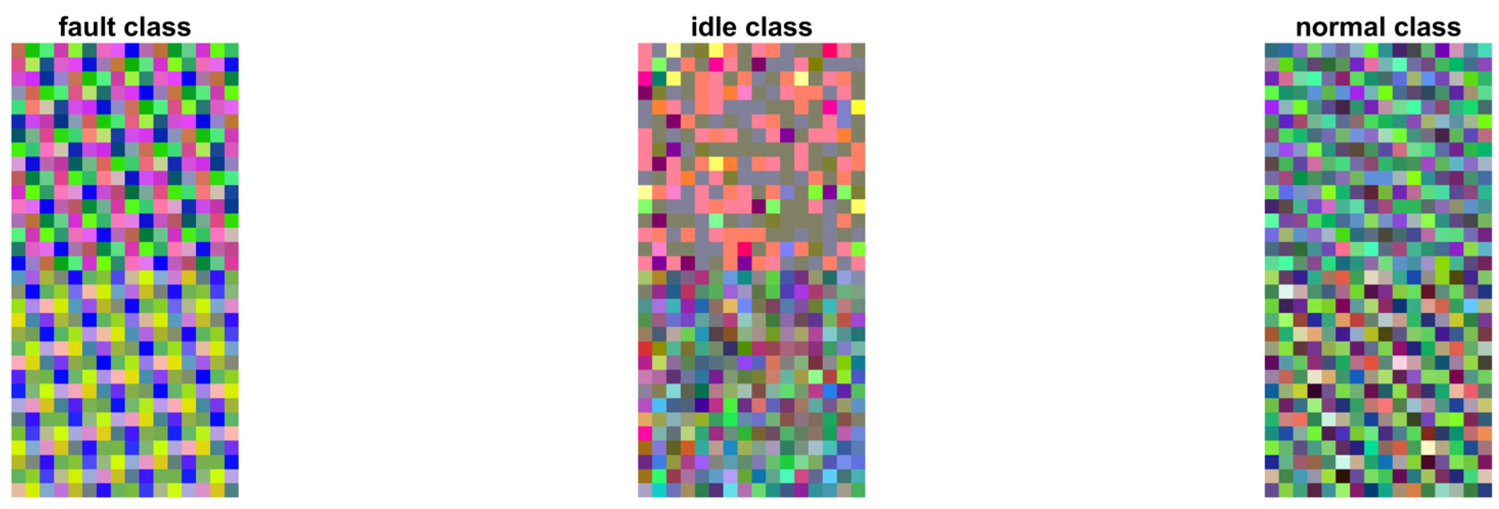
This method, named IMU6DoF-Time2RGBbyType-CNN, directly converts the time series data for each axis (X, Y, and Z) of the IMU sensor into separate channels of an RGB image. This creates a single image where the red channel represents the X-axis data, the green channel represents the Y-axis data, and the blue channel represents the Z-axis data. The resulting RGB image is then fed into a convolutional neural network (CNN) for classification. Figure 12 shows representative input images for each class (idle, normal operation, and fault). As can be seen, the top half of the image corresponds to the accelerometer data (red, green, blue channels for X, Y, and Z), while the bottom half corresponds to the gyroscope data (again, red, green, and blue for X, Y, and Z).
Similar to the IMU6DoF-Time2GrayscaleGrid-CNN method (Figure 9), the training progress of the CNN used in the IMU6DoF-Time2RGBbyType-CNN method can be visualized (Figure 13) using a graph that plots training loss and accuracy over epochs. The data has been zoomed in to focus on the first 500 iterations for a clearer comparison between the two methods. Figure 13 reveals interesting insights into the training behavior of the CNNs for both approaches. It is evident that the IMU6DoF-Time2GrayscaleGrid-CNN method achieves a training accuracy exceeding 95% faster than the IMU6DoF-Time2RGBbyType-CNN method does. This observation suggests that the CNN trained on the simpler grayscale image representation might converge into a good solution more efficiently compared to the model handling the RGB color image.
The performance of the IMU6DoF-Time2RGBbyType-CNN method can be further evaluated using a confusion matrix, shown in Figure 14. Similar to the confusion matrix described for the grayscale method (Section 4.1), this matrix is a table with rows representing the true classes (idle, normal, fault) and columns representing the predicted classes. The IMU6DoF-Time2RGBbyType-CNN and IMU6DoF-Time2GrayscaleGrid-CNN models have similar accuracy around 100%.
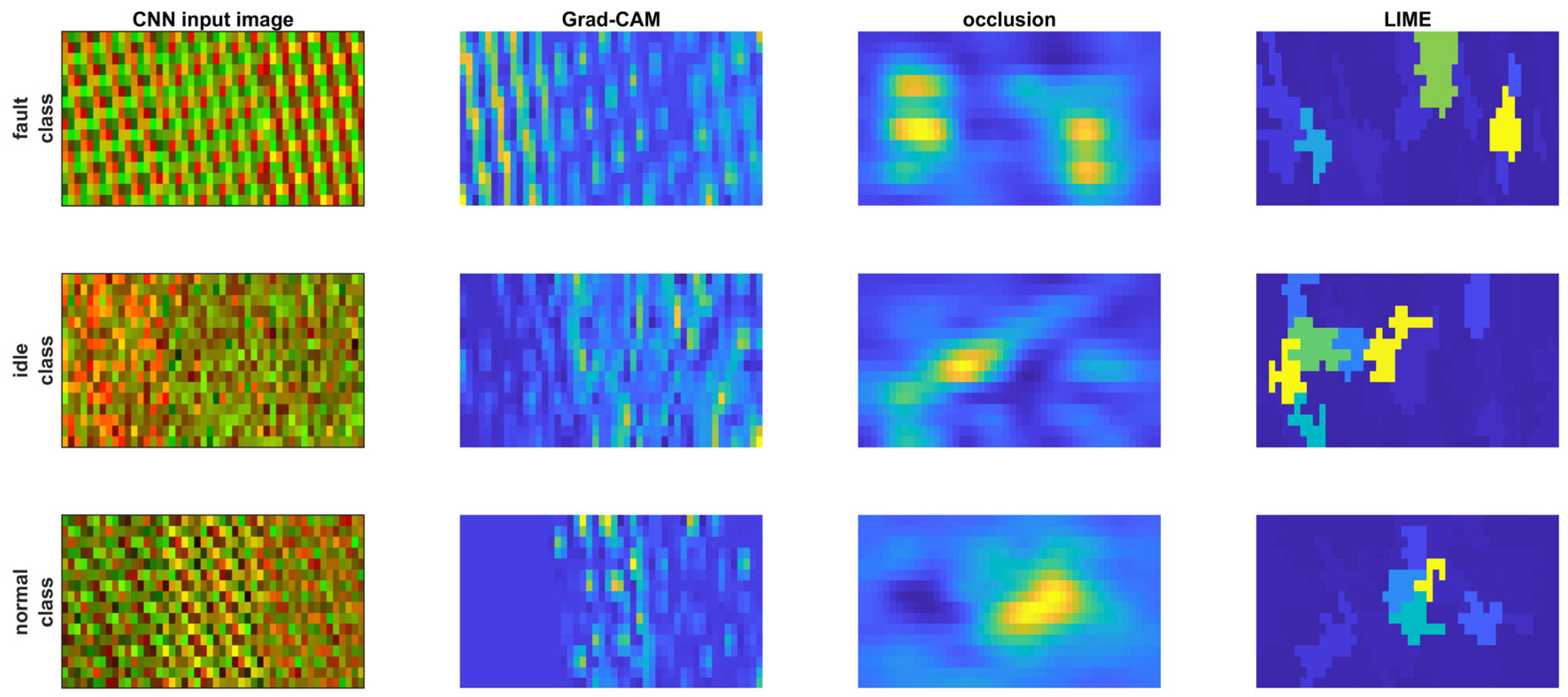
Convolutional neural networks (CNNs) are powerful tools for image recognition, but their inner workings can be difficult to interpret. This makes it challenging to understand how a CNN arrives at its classification decisions. In the provided Figure 15, the first column shows the input RGB image. Similar to Section 4.1, the rows correspond to the classes of fault, idle, and normal, respectively. Techniques like Grad-CAM, occlusion sensitivity, and LIME were used to aid in CNN interpretability. These methods provide visualizations that highlight the regions of the image that the CNN focuses on for classification. By analyzing these visualizations, researchers can gain insights into the decision-making process of the CNN and understand how it differentiates between different classes. Frequency domain analysis (as shown in Figure 7) reveals a characteristic signature of the fault condition. This signature is characterized by a dominant peak at 20 Hz, specifically present in the X-axis of the accelerometer data and the Z-axis of the gyroscope data. The Grad-CAM and occlusion sensitivity analysis for the IMU6DoF-Time2RGBbyType-CNN method point towards the gyroscope data as a dominant factor in distinguishing fault conditions. These techniques highlight specific features or channels within the RGB image representation that correspond to the gyroscope data (particularly the Z-axis), suggesting that the CNN heavily relies on information from the gyroscope for accurate fault classification.
4.3. The IMU6DoF-Time2RGBbyAxis-CNN Method
The method named IMU6DoF-Time2RGBbyAxis-CNN adopts a unique approach to transform time series data from a 6DoF IMU sensor into a format suitable for image-based recognition using a convolutional neural network (CNN). A crucial aspect of this method is the alignment of data across axes. By segmenting and reshaping data windows to be the same size for each axis (X, Y), the IMU6DoF-Time2RGBbyAxis-CNN model ensures that corresponding time points from different axes are positioned together within the RGB image. This alignment potentially allows the CNN to learn the relationships between the movements along different axes, which might be beneficial for classification. Representative input images for each class (idle, normal operation, and fault) generated using this method can be seen in Figure 16. The figure clearly illustrates that the left of the image contains the accelerometer X-axis and gyroscope X-axis data, the middle part contains the accelerometer Y-axis and gyroscope Y-axis data, and the right part of the image represents the accelerometer Z-axis and gyroscope Z-axis data; moreover, the blue channel was set to zero.
Similar to the IMU6DoF-Time2GrayscaleGrid-CNN method (Figure 9), the training progress of the CNNs used in both IMU6DoF-Time2RGBbyType-CNN (Figure 13) and IMU6DoF-Time2RGBbyAxis-CNN can be visualized using graphs that plot training loss and accuracy over epochs. The data in Figure 17 has been zoomed in to the first 500 iterations for a clearer comparison between the three methods. The training progress reveals interesting insights. As observed previously, the IMU6DoF-Time2GrayscaleGrid-CNN method achieves a training accuracy exceeding 95% faster than the IMU6DoF-Time2RGBbyType-CNN method does. This suggests that the simpler grayscale image representation might be easier for the CNN to learn from compared to the RGB-by-type approach. The IMU6DoF-Time2RGBbyAxis-CNN method (which utilizes axis-aligned data representations in the RGB image) is not trained as fast as the grayscale method; however, it achieves faster convergence than the IMU6DoF-Time2RGBbyType-CNN method. This is because the axis-aligned representation in RGB by axis inherently captures some relationships between the axes (as data points from the same time window are positioned together), potentially simplifying the learning process for the CNN compared to the more abstract feature vector used in RGB by type.
Similar to the evaluation methods used for the other CNN approaches, the performance of the IMU6DoF-Time2RGBbyAxis-CNN method can be assessed using a confusion matrix as shown in Figure 18. It is noteworthy that, as previously mentioned, IMU6DoF-Time2GrayscaleGrid-CNN, IMU6DoF-Time2RGBbyType-CNN, and IMU6DoF-Time2RGBbyAxis-CNN each achieved a high accuracy of around 100%.
Understanding how the CNN in the IMU6DoF-Time2RGBbyAxis-CNN method makes decisions is crucial for building trust and potentially improving the model. Techniques like Grad-CAM can be applied to visualize the regions within the RGB image that the CNN focuses on when classifying a specific operational state (idle, normal, fault), as shown in Figure 19. Since the method uses an axis-aligned representation, these visualizations might highlight specific areas within a channel that correspond to movements along a particular axis. For example, at the fault class, Grad-CAM highlights in the red channel for X-axis movements in the accelerometer data and movements in the green channel for the Z-axis in the gyroscope data. This alignment can potentially offer more intuitive insights into the features the CNN learns compared to other RGB representation methods, as the highlighted regions directly relate to specific axes. In essence, by combining Grad-CAM visualizations with occlusion sensitivity analysis, we can achieve a more comprehensive understanding of how the IMU6DoF-Time2RGBbyAxis-CNN method leverages the axis-aligned data representation in the RGB image. This combined analysis helps to see how the model effectively distinguishes between different operational states based on the sensor data from the specific axes highlighted by Grad-CAM.
5. Discussion
The comparison of the proposed methods was conducted in the high-performance computing environment of a remote virtual machine provided by the Poznan University of Technology. The system utilized VMware for virtualization and offered 16 GB of RAM for efficient memory management. The processing power was provided by an AMD EPYC 7402 processor, with two cores and four threads specifically allocated for this task. It is important to note that the CNN training was processed entirely on the CPU for a controlled comparison. The software environment used for this research was MathWorks MATLAB R2023a, which provided the necessary tools for data processing, image generation, CNN implementation, and performance evaluation.
A paper clip attached to a fan blade can be a valid representation of a real fault for proof-of-concept purposes, but with limitations. In this paragraph, we discuss the limitations of this approach while exploring real-world examples of fan blade imbalance in computer and duct fan applications. This approach induces an imbalance that manifests itself as an increased vibration, mimicking the signature of a genuine fault. Vibration sensors can then detect these changes, allowing the researcher to evaluate the ability of the IMU6DoF-Time2GrayscaleGrid-CNN, IMU6DoF-Time2RGBbyType-CNN, and IMU6DoF-Time2RGBbyAxis-CNN methods to identify such imbalances through vibration analysis. However, it is crucial to acknowledge the limitations of this method. A paper clip represents a highly specific type and degree of imbalance. Real-world fan blade failures can manifest in numerous ways with varying severities. The paper clip might not adequately capture the full spectrum of potential imbalances encountered in practical applications. Real-world imbalances can arise from manufacturing defects (for example, uneven blade mass distribution), physical damage (for example, bent or cracked blades), or foreign object accumulation on a blade. These factors can lead to imbalances that differ significantly from the simple addition of mass introduced by a paper clip. The paper clip induces a moderate level of imbalance. However, real-world faults can range from very slight imbalances, which might not be readily detectable, to severe imbalances that cause significant vibration and rapid equipment degradation. A computer fan experiencing blade imbalance typically exhibits increased noise levels, vibrations detectable in the computer case, and potentially unstable fan speeds. In severe cases, the imbalance can lead to premature fan failure or damage to the mounting bracket. The computer fan imbalance can be caused by manufacturing defects, physical damage to a blade (e.g., a bent tip), or the accumulation of dust on one side of the blade, which can all contribute to imbalance in computer fans. Similarly to computer fans, a duct fan with an imbalanced blade will experience increased vibrations and noise levels within the duct system. This can disrupt airflow patterns, reduce efficiency, and potentially damage the ductwork due to excessive vibrations. Similar to computer fans, imbalance can be caused by manufacturing defects, physical damage (e.g., a bent or cracked blade), or debris buildup on a blade, and these can all lead to imbalance in duct fans. Additionally, the misalignment of the fan within the duct can also cause vibration issues. Introducing an imbalance into a fan system using a paper clip attached to an blade is a appropriate method for proof-of-concept studies at low technology readiness levels (TRLs) related to basic research [32]. In this regard, each proposed method (IMU6DoF-Time2GrayscaleGrid-CNN, IMU6DoF-Time2RGBbyType-CNN, and IMU6DoF-Time2RGBbyAxis-CNN) itself is under investigation, placing it at a relatively low TRL. While the methods are currently under development (low TRLs), significant progress can be made to elevate their TRLs towards those of real-world application (TRLs 7–9), which are equivalent to development work (product development at business). The roadmap of technology readiness at TRL 7 assumes that the demonstration of the system prototype in an operational environment was successful. Next, the prototype testing is moved to a more realistic operational environment, involving functional computer systems or dedicated fan test stands. The final level is TRL 9, which means that the actual system was successfully tested in an operational environment. This requires the final system to be deployed in real-world industrial settings for extended periods. This allows for real-world data collection and performance evaluation under practical operating conditions. In addition, system performance is monitored and data are gathered on its effectiveness in detecting fan blade imbalance and preventing equipment failures. By progressing through this TRL roadmap, the proposed methods have the potential to reach a high TRL level (TRLs 7–9) and become valuable tools for preventive maintenance and improving equipment reliability in various industrial applications. This manuscript was focused at a low TRL which allows for a positive verification of the proof of concept of the proposed methods. The comparison of the training progress of the proposed methods is illustrated in Table 1, highlighting the number of epochs required for each method to reach a desired level of accuracy. Additionally, Table 2 provides insights into the image generation efficiency of each method, which directly impacts the overall processing time for fault diagnosis. The reference methods (STFTx6-CNN [1] and CWTx6-CNN [31]) achieved perfect validation accuracy (100%), and their training times of several minutes are significantly faster compared to the those of the proposed methods, which had training speeds exceeding 30 min (IMU6DoF-Time2GrayscaleGrid-CNN, IMU6DoF-Time2RGBbyType-CNN, and IMU6DoF-Time2RGBbyAxis-CNN). Additionally, the reference methods achieved over 90% convergence after five iterations, whereas the proposed methods require 60 to 150 iterations for similar accuracy. However, this trade-off comes with a substantial benefit in terms of computational efficiency. The proposed methods offer significantly faster execution times, processing a segment of 256 samples by 6 axes of sensors in less than half a millisecond. This is a considerable improvement compared to the reference methods, which require around 9 milliseconds for STFT with 128 × 6 segments and a slow 29 milliseconds for CWT with 96 × 6 segments. In real-world applications, especially those involving time-critical fault detection, the faster processing speeds offered by the proposed methods become a major advantage. While all methods achieve excellent classification accuracy, the ability to perform computations in less than a millisecond makes the proposed methods more suitable for online monitoring and real-time decision making. Future work can explore techniques to further optimize the training process of the proposed methods while potentially leveraging interpretability techniques like Grad-CAM to gain deeper insights into the features learned by the CNNs for even more robust fault classification.
In real-world applications, it is essential to trust the model’s predictions. Interpretability techniques can help us understand the reasoning behind the CNN’s decisions, fostering confidence in its performance. Future research can explore advanced interpretability techniques specifically designed for image-based CNNs used in sensor-based fault diagnosis. Additionally, analytic analysis can be conducted to evaluate the effectiveness of these techniques in conveying the model’s reasoning to domain experts.
The vibration signals in Figure 6 appear to be visually distinct under certain operating conditions; human interpretation can be subjective and may not capture the full spectrum of informative features present in the data. The proposed methods leverage the power of CNNs to address this challenge and achieve more robust and generalizable fault classification. CNNs excel at automatically extracting relevant features from complex data patterns. By training the CNN on a diverse dataset of vibration signals representing various severities and other potential faults, the model learns to identify these subtle features and classify them accurately. Traditional machine learning approaches often require extensive manual feature engineering. CNNs can learn features directly from the raw data, reducing development time and potential human bias in feature selection. Furthermore, the previous research stage under six-switch and three-phase (6S3P) topology inverter faults [12], shows insights that phase currents can be converted into images for fault diagnosis and recognized more accurately than other classifiers (e.g., decision trees, naive Bayes, SVMs (support vector machines), KNN (k-nearest neighbors) or narrow neural networks) despite the fact that the phase currents were visually different. The insights from the previous research on 6S3P inverter faults provide strong support for the proposed approach of leveraging CNNs for fan blade imbalance detection. By automatically extracting complex features from vibration data, the IMU6DoF-Time2GrayscaleGrid-CNN, IMU6DoF-Time2RGBbyType-CNN and IMU6DoF-Time2RGBbyAxis-CNN methods have the potential to achieve superior fault classification accuracy and robustness compared to simpler methods, even when some level of visual distinction might be present in the raw data.
In the case of the IMU6DoF-Time2GrayscaleGrid-CNN method, Grad-CAM highlights specific areas within the grayscale image corresponding to the fault class shown in Figure 11. For instance, these highlighted regions could be located in the top-left corner (corresponding to the X-axis of the accelerometer) and the bottom-right corner (corresponding to the Z-axis of the gyroscope) of the image. This visual cue aligns with the knowledge that the fault condition is characterized by a dominant frequency of 20 Hz in both the X-axis accelerometer and Z-axis gyroscope data (as shown in Figure 7). By highlighting these specific areas, Grad-CAM helps us to understand that the CNN focuses on data patterns related to these axes when identifying the fault. The IMU6DoF-Time2RGBbyType-CNN method does not provide a direct visual representation of the data like the other frequency domain methods (STFTx6-CNN and CWTx6-CNN); however, interpretability techniques like Grad-CAM can still be applied to an input image as shown in Figure 15. By analyzing the results of Grad-CAM, we can gain insights into which features within the image hold the most significance for the CNN’s decision-making process. If the Grad-CAM analysis consistently highlights an image area heavily influenced by the gyroscope data, particularly the Z-axis, it might suggest that these movements play a key role in differentiating the fault class from other operational states. The interpretability of this method allows us to underline and select one dominant sensor for the future optimization of data acquisition and data processing. The IMU6DoF-Time2RGBbyAxis-CNN method benefits from its axis-aligned representation within the RGB image. In this case, Grad-CAM visualizations offer intuitive interpretations, as shown in Figure 19. For example, for the fault class, Grad-CAM highlights movements along the X-axis in the accelerometer data and movements along the Z-axis in the gyroscope data. This direct mapping between data and axes in the image makes the interpretation of Grad-CAM results more straightforward. Which axes are most influential for the CNN’s decision in the fault class can be directly seen, aligning with the understanding that the fault involves vibrations in both the X and Z directions.
The selection of the 200 Hz sampling frequency was arbitrary and should be chosen appropriately for other applications in which the proposed method will be applied. The system was preliminary investigated at 100 Hz, 200 Hz, 400 Hz, 500 Hz, and 2000 Hz sampling frequencies and 200 Hz was selected, in which frequency components are rich. In previous research investigations for mechanical vibrations in direct motor drives, up to 10,000 Hz samplings of a, b, c currents with multiple mechanical resonances were conducted [33,34,35]. However, the proof of concept which verifies if the idea is feasible does not require a sufficiently high sampling frequency; therefore, 200 Hz was a wise selection. The number of collected samples is several times smaller, allowing the proof of concept to be carried out with less computational resources. The sampling period was selected to achieve an image of the same size of 16 × 16 pixels, which is equivalent to 256 samples for the single axis. The system was preliminary investigated for 11 × 11, 12 × 12 and 16 × 16 pixels. The second condition was to achieve taking around one second to capture at least one period of low-frequency components.
The proposed methods (IMU6DoF-Time2GrayscaleGrid-CNN, IMU6DoF-Time2RGBbyType-CNN, and IMU6DoF-Time2RGBbyAxis-CNN) were validated using a modified demonstrator (Figure 20) in a second scenario involving different fan velocities and a 12V DC supply. The demonstrator in Figure 4 was extended with a P-channel MOSFET (metal oxide semiconductor field effect transistor) to control the fan velocity in 10% increments from 10% to 100% of its nominal speed. Additionally, a second paper clip was introduced to simulate a different fault condition. The sampling frequency was set to 2000 Hz for this scenario. The partial images were reshaped from 576 samples to a size of 24 × 24 pixels. These data were used to evaluate the performance of the proposed methods. Label fault 1 (or fault) was defined as having one paper clip attached and fault 2 (or fault2) represented having two paper clips attached. Images of the IMU6DoF-Time2GrayscaleGrid-CNN method are shown in Figure 21, Figure 22 shows example input images for the IMU6DoF-Time2RGBbyType-CNN method, and Figure 23 shows example images for the IMU6DoF-Time2RGBbyAxis-CNN method. A total of 1230 images were generated for each velocity level, resulting in a dataset of 36,900 images per method (1230 images/velocity × 10 velocities × 3 class). This dataset was then divided, with 80% being allocated to train CNN models and 20% being used for validation.
The training process for the second scenario, involving different fan velocities, took between 233 min (approximately 3.9 h) and 265 min (slightly over 4.4 h). The training progress curves (Figure 24) mirrored the observations from the first scenario. As previously noted, the IMU6DoF-Time2GrayscaleGrid-CNN method achieved training accuracy faster than the IMU6DoF-Time2RGBbyType-CNN method did. The confusion matrices for each method after training are presented in Figure 25, Figure 26 and Figure 27. The final validation accuracy ranged from 99.88% (Figure 25 and Figure 27) to 99.97% (Figure 26), with the IMU6DoF-Time2RGBbyType-CNN method achieving the highest accuracy. However, these differences are not statistically significant. The results demonstrate that the proposed methods can achieve high accuracies for fault classification even with more complex datasets. However, the complexity of the data significantly impacts the training time. The first scenario, featuring a constant velocity, allowed for faster training compared to the second scenario involving varying velocities. In scenario two, training each method required approximately four hours (around 12 h total—around half a day), which is considerably longer than the training time observed in the first scenario with a constant velocity (around 30 min per method). This highlights the potential benefit of utilizing simpler datasets during the initial proof-of-concept stage of model development. This approach facilitates faster training and initial validation. Subsequently, the model can be validated on more complex datasets that incorporate real-world variations, ensuring its robustness in practical applications.
The fan is often installed inside enclosures. There are potential impacts of enclosures on vibration frequencies in research on fan blade imbalance detection using the IMU6DoF-Time2GrayscaleGrid-CNN, IMU6DoF-Time2RGBbyType-CNN, and IMU6DoF-Time2RGBbyAxis-CNN methods. This raises an excellent point and vibration frequencies can indeed be altered when a fan is installed inside an enclosure. The enclosure can act as a resonator, amplifying certain vibration frequencies while damping others. This can potentially change the dominant frequencies observed in the vibration data compared to those of a freestanding fan. The mounting method and the rigidity of the enclosure can influence how the vibrations of the fan are transmitted to the sensors. This can introduce additional complexity into the vibration signal. In future work at higher TRLs, it is planned to expand experiments beyond isolated fan setups. Future work will incorporate tests with fans mounted within enclosures that are representative of real-world applications and will be more related to the higher TRLs of a possible business product. This will allow researchers to analyze how enclosure effects influence the vibration signatures of imbalanced blades.
An important question is the economic viability of using the proposed methods for monitoring a low-cost fan such as the Yate Loon Electronics model, and it is crucial to clarify the context of research at this stage. The current work primarily focuses on establishing the proof of concept for the IMU6DoF-Time2GrayscaleGrid-CNN, IMU6DoF-Time2RGBbyType-CNN, and IMU6DoF-Time2RGBbyAxis-CNN methods in detecting fan blade imbalance. This initial development stage (at a low technology readiness level, TRL) prioritizes demonstrating the technical feasibility of the method. The Yate Loon fan serves as a readily available and well-defined test platform for this purpose. The point regarding economic feasibility becomes highly relevant when considering higher TRLs (TRLs 7–9). At these stages, the focus shifts towards developing a commercially viable product suitable for real-world applications. The economic viability depends on the target application. Although a low-cost fan like the Yate Loon model might not warrant such a system due to its low replacement cost, the method used could be highly cost-effective for high-value equipment where fan failure can lead to significant downtime and production losses. Examples include industrial fans in critical cooling systems, large server fans in data centers, or high-performance fans in wind turbines. As there is a trend towards higher TRLs, the technology can be designed to be scalable and adaptable. This could involve developing modular sensor units or offering different levels of services depending on the specific needs and budget constraints of the customer. Although the economic feasibility of the method for a low-cost fan such as the Yate Loon model might be limited at this stage, the core technology holds promise for providing a cost-effective solution for critical equipment in various industrial applications. As the move towards higher TRLs is made, economic considerations will become a central focus in developing a commercially viable product.
6. Conclusions
This investigation explored three image-based approaches for machine fault diagnosis using data from a 6DOF IMU sensor. All three methods achieved high accuracy in classifying operational states (idle, normal, fault). The IMU6DoF-Time2GrayscaleGrid-CNN method, which converts time series data into a single grayscale image, demonstrated the fastest training convergence. However, the methods utilizing RGB representations, like the IMU6DoF-Time2RGBbyType-CNN and IMU6DoF-Time2RGBbyAxis-CNN methods, might offer additional insights. While IMU6DoF-Time2RGBbyType-CNN utilizes features extracted from the data, IMU6DoF-Time2RGBbyAxis-CNN leverages an axis-aligned representation within the RGB image. This alignment potentially allows the CNN in IMU6DoF-Time2RGBbyAxis-CNN to learn relationships between movements along different axes, which might be beneficial for classification. Additionally, the axis-aligned representation in the Grad-CAM visualizations for IMU6DoF-Time2RGBbyAxis-CNN could provide more intuitive explanations for the CNN’s decisions compared to other methods. Further research can explore the effectiveness of these interpretability techniques and potentially combine them with domain knowledge to refine the understanding of the features learned by the CNNs for robust fault classification.
Funding
This research was funded by the Poznan University of Technology, grant number 0214/SBAD/0249.
Data Availability Statement
Data are contained within the article.
Conflicts of Interest
The author declares no conflicts of interest.
References
- Łuczak, D.; Brock, S.; Siembab, K. Cloud Based Fault Diagnosis by Convolutional Neural Network as Time–Frequency RGB Image Recognition of Industrial Machine Vibration with Internet of Things Connectivity. Sensors 2023, 23, 3755. [Google Scholar] [CrossRef] [PubMed]
- Chen, H.-Y.; Lee, C.-H. Vibration Signals Analysis by Explainable Artificial Intelligence (XAI) Approach: Application on Bearing Faults Diagnosis. IEEE Access 2020, 8, 134246–134256. [Google Scholar] [CrossRef]
- Wang, Y.; Yang, M.; Li, Y.; Xu, Z.; Wang, J.; Fang, X. A Multi-Input and Multi-Task Convolutional Neural Network for Fault Diagnosis Based on Bearing Vibration Signal. IEEE Sens. J. 2021, 21, 10946–10956. [Google Scholar] [CrossRef]
- Rauber, T.W.; da Silva Loca, A.L.; de Assis Boldt, F.; Rodrigues, A.L.; Varejão, F.M. An Experimental Methodology to Evaluate Machine Learning Methods for Fault Diagnosis Based on Vibration Signals. Expert Syst. Appl. 2021, 167, 114022. [Google Scholar] [CrossRef]
- Meyer, A. Vibration Fault Diagnosis in Wind Turbines Based on Automated Feature Learning. Energies 2022, 15, 1514. [Google Scholar] [CrossRef]
- Li, Z.; Zhang, Y.; Abu-Siada, A.; Chen, X.; Li, Z.; Xu, Y.; Zhang, L.; Tong, Y. Fault Diagnosis of Transformer Windings Based on Decision Tree and Fully Connected Neural Network. Energies 2021, 14, 1531. [Google Scholar] [CrossRef]
- Gao, S.; Xu, L.; Zhang, Y.; Pei, Z. Rolling Bearing Fault Diagnosis Based on SSA Optimized Self-Adaptive DBN. ISA Trans. 2022, 128, 485–502. [Google Scholar] [CrossRef]
- Wang, C.-S.; Kao, I.-H.; Perng, J.-W. Fault Diagnosis and Fault Frequency Determination of Permanent Magnet Synchronous Motor Based on Deep Learning. Sensors 2021, 21, 3608. [Google Scholar] [CrossRef]
- Feng, Z.; Gao, A.; Li, K.; Ma, H. Planetary Gearbox Fault Diagnosis via Rotary Encoder Signal Analysis. Mech. Syst. Signal Process. 2021, 149, 107325. [Google Scholar] [CrossRef]
- Ma, J.; Li, C.; Zhang, G. Rolling Bearing Fault Diagnosis Based on Deep Learning and Autoencoder Information Fusion. Symmetry 2022, 14, 13. [Google Scholar] [CrossRef]
- Huang, W.; Du, J.; Hua, W.; Lu, W.; Bi, K.; Zhu, Y.; Fan, Q. Current-Based Open-Circuit Fault Diagnosis for PMSM Drives With Model Predictive Control. IEEE Trans. Power Electron. 2021, 36, 10695–10704. [Google Scholar] [CrossRef]
- Łuczak, D.; Brock, S.; Siembab, K. Fault Detection and Localisation of a Three-Phase Inverter with Permanent Magnet Synchronous Motor Load Using a Convolutional Neural Network. Actuators 2023, 12, 125. [Google Scholar] [CrossRef]
- Jiang, L.; Deng, Z.; Tang, X.; Hu, L.; Lin, X.; Hu, X. Data-Driven Fault Diagnosis and Thermal Runaway Warning for Battery Packs Using Real-World Vehicle Data. Energy 2021, 234, 121266. [Google Scholar] [CrossRef]
- Chang, C.; Zhou, X.; Jiang, J.; Gao, Y.; Jiang, Y.; Wu, T. Electric Vehicle Battery Pack Micro-Short Circuit Fault Diagnosis Based on Charging Voltage Ranking Evolution. J. Power Sources 2022, 542, 231733. [Google Scholar] [CrossRef]
- Wang, Z.; Tian, B.; Qiao, W.; Qu, L. Real-Time Aging Monitoring for IGBT Modules Using Case Temperature. IEEE Trans. Ind. Electron. 2016, 63, 1168–1178. [Google Scholar] [CrossRef]
- Dhiman, H.S.; Deb, D.; Muyeen, S.M.; Kamwa, I. Wind Turbine Gearbox Anomaly Detection Based on Adaptive Threshold and Twin Support Vector Machines. IEEE Trans. Energy Convers. 2021, 36, 3462–3469. [Google Scholar] [CrossRef]
- Cao, Y.; Sun, Y.; Xie, G.; Li, P. A Sound-Based Fault Diagnosis Method for Railway Point Machines Based on Two-Stage Feature Selection Strategy and Ensemble Classifier. IEEE Trans. Intell. Transp. Syst. 2022, 23, 12074–12083. [Google Scholar] [CrossRef]
- Shiri, H.; Wodecki, J.; Ziętek, B.; Zimroz, R. Inspection Robotic UGV Platform and the Procedure for an Acoustic Signal-Based Fault Detection in Belt Conveyor Idler. Energies 2021, 14, 7646. [Google Scholar] [CrossRef]
- Karabacak, Y.E.; Gürsel Özmen, N.; Gümüşel, L. Intelligent Worm Gearbox Fault Diagnosis under Various Working Conditions Using Vibration, Sound and Thermal Features. Appl. Acoust. 2022, 186, 108463. [Google Scholar] [CrossRef]
- Maruyama, T.; Maeda, M.; Nakano, K. Lubrication Condition Monitoring of Practical Ball Bearings by Electrical Impedance Method. Tribol. Online 2019, 14, 327–338. [Google Scholar] [CrossRef]
- Wakiru, J.M.; Pintelon, L.; Muchiri, P.N.; Chemweno, P.K. A Review on Lubricant Condition Monitoring Information Analysis for Maintenance Decision Support. Mech. Syst. Signal Process. 2019, 118, 108–132. [Google Scholar] [CrossRef]
- Zhou, Q.; Chen, R.; Huang, B.; Liu, C.; Yu, J.; Yu, X. An Automatic Surface Defect Inspection System for Automobiles Using Machine Vision Methods. Sensors 2019, 19, 644. [Google Scholar] [CrossRef] [PubMed]
- Yang, L.; Fan, J.; Liu, Y.; Li, E.; Peng, J.; Liang, Z. A Review on State-of-the-Art Power Line Inspection Techniques. IEEE Trans. Instrum. Meas. 2020, 69, 9350–9365. [Google Scholar] [CrossRef]
- Davari, N.; Akbarizadeh, G.; Mashhour, E. Intelligent Diagnosis of Incipient Fault in Power Distribution Lines Based on Corona Detection in UV-Visible Videos. IEEE Trans. Power Deliv. 2021, 36, 3640–3648. [Google Scholar] [CrossRef]
- Kim, S.; Kim, D.; Jeong, S.; Ham, J.-W.; Lee, J.-K.; Oh, K.-Y. Fault Diagnosis of Power Transmission Lines Using a UAV-Mounted Smart Inspection System. IEEE Access 2020, 8, 149999–150009. [Google Scholar] [CrossRef]
- Ullah, Z.; Lodhi, B.A.; Hur, J. Detection and Identification of Demagnetization and Bearing Faults in PMSM Using Transfer Learning-Based VGG. Energies 2020, 13, 3834. [Google Scholar] [CrossRef]
- Long, H.; Xu, S.; Gu, W. An Abnormal Wind Turbine Data Cleaning Algorithm Based on Color Space Conversion and Image Feature Detection. Appl. Energy 2022, 311, 118594. [Google Scholar] [CrossRef]
- Xie, T.; Huang, X.; Choi, S.-K. Intelligent Mechanical Fault Diagnosis Using Multisensor Fusion and Convolution Neural Network. IEEE Trans. Ind. Inform. 2022, 18, 3213–3223. [Google Scholar] [CrossRef]
- Zhou, Y.; Wang, H.; Wang, G.; Kumar, A.; Sun, W.; Xiang, J. Semi-Supervised Multiscale Permutation Entropy-Enhanced Contrastive Learning for Fault Diagnosis of Rotating Machinery. IEEE Trans. Instrum. Meas. 2023, 72, 1–10. [Google Scholar] [CrossRef]
- Xu, M.; Gao, J.; Zhang, Z.; Wang, H. Bearing-Fault Diagnosis with Signal-to-RGB Image Mapping and Multichannel Multiscale Convolutional Neural Network. Entropy 2022, 24, 1569. [Google Scholar] [CrossRef] [PubMed]
- Łuczak, D. Machine Fault Diagnosis through Vibration Analysis: Continuous Wavelet Transform with Complex Morlet Wavelet and Time–Frequency RGB Image Recognition via Convolutional Neural Network. Electronics 2024, 13, 452. [Google Scholar] [CrossRef]
- OECD. Frascati Manual 2015-Guidelines for Collecting and Reporting Data on Research and Experimental Development; The Measurement of Scientific, Technological and Innovation Activities; OECD Publishing: Paris, France, 2015; ISBN 978-926423901-2. [Google Scholar] [CrossRef]
- Łuczak, D. Mechanical Vibrations Analysis in Direct Drive Using CWT with Complex Morlet Wavelet. Power Electron. Drives 2023, 8, 65–73. [Google Scholar] [CrossRef]
- Łuczak, D. Nonlinear Identification with Constraints in Frequency Domain of Electric Direct Drive with Multi-Resonant Mechanical Part. Energies 2021, 14, 7190. [Google Scholar] [CrossRef]
- Brock, S.; Luczak, D.; Nowopolski, K.; Pajchrowski, T.; Zawirski, K. Two Approaches to Speed Control for Multi-Mass System with Variable Mechanical Parameters. IEEE Trans. Ind. Electron. 2016, 64, 3338–3347. [Google Scholar] [CrossRef]
Figure 1.
The proposed method, named IMU6DoF-Time2GrayscaleGrid-CNN, as a grid of six grayscale images of 16-by-16 pixels recognized by s CNN with a given architecture.
Figure 1.
The proposed method, named IMU6DoF-Time2GrayscaleGrid-CNN, as a grid of six grayscale images of 16-by-16 pixels recognized by s CNN with a given architecture.

Figure 2.
The proposed method, named IMU6DoF-Time2RGBbyType-CNN, with sub-images of 16-by-16 pixels aligned by sensor type and recognized by a CNN with a given architecture.
Figure 2.
The proposed method, named IMU6DoF-Time2RGBbyType-CNN, with sub-images of 16-by-16 pixels aligned by sensor type and recognized by a CNN with a given architecture.

Figure 3.
The proposed method, named IMU6DoF-Time2RGBbyAxis-CNN, with sub-images of 16-by-16 pixels aligned by axis and recognized by a CNN with a given architecture.
Figure 3.
The proposed method, named IMU6DoF-Time2RGBbyAxis-CNN, with sub-images of 16-by-16 pixels aligned by axis and recognized by a CNN with a given architecture.

Figure 4.
Microcontroller-based demonstrator of machine fault diagnosis.

Figure 5.
Data transmission via MQTT.

Figure 6.
Time series data in one segment of 256 samples for the three axes of the accelerometer and gyroscope.
Figure 6.
Time series data in one segment of 256 samples for the three axes of the accelerometer and gyroscope.

Figure 7.
The single-segment time series data for each class converted into frequency domains for the three axes of the accelerometer and the three axes of the gyroscope.
Figure 7.
The single-segment time series data for each class converted into frequency domains for the three axes of the accelerometer and the three axes of the gyroscope.

Figure 8.
Greyscale images for each class of the IMU6DoF-Time2GrayscaleGrid-CNN method.

Figure 9.
The training progress of the CNN for the IMU6DoF-Time2GrayscaleGrid-CNN method.

Figure 10.
The matrix of confusion after training IMU6DoF-Time2GrayscaleGrid-CNN (training—left; testing—right).
Figure 10.
The matrix of confusion after training IMU6DoF-Time2GrayscaleGrid-CNN (training—left; testing—right).

Figure 11.
The interpretability of the proposed IMU6DoF-Time2GrayscaleGrid-CNN method.

Figure 12.
The RGB image for each class of the IMU6DoF-Time2RGBbyType-CNN method.

Figure 13.
The training progress of the CNN for the IMU6DoF-Time2RGBbyType-CNN method compared with that of the IMU6DoF-Time2GrayscaleGrid-CNN method (training—left; validation—right).
Figure 13.
The training progress of the CNN for the IMU6DoF-Time2RGBbyType-CNN method compared with that of the IMU6DoF-Time2GrayscaleGrid-CNN method (training—left; validation—right).

Figure 14.
The matrix of confusion after training IMU6DoF-Time2RGBbyType-CNN (training—left; testing—right).
Figure 14.
The matrix of confusion after training IMU6DoF-Time2RGBbyType-CNN (training—left; testing—right).

Figure 15.
Interpretability of the proposed IMU6DoF-Time2RGBbyType-CNN method.

Figure 16.
The RGB image for each class of the IMU6DoF-Time2RGBbyAxis-CNN method.

Figure 17.
The training progress of the CNN of IMU6DoF-Time2RGBbyAxis-CNN compared with the that of IMU6DoF-Time2GrayscaleGrid-CNN and that of IMU6DoF-Time2RGBbyType-CNN (training—left; validation—right).
Figure 17.
The training progress of the CNN of IMU6DoF-Time2RGBbyAxis-CNN compared with the that of IMU6DoF-Time2GrayscaleGrid-CNN and that of IMU6DoF-Time2RGBbyType-CNN (training—left; validation—right).

Figure 18.
The matrix of confusion after training IMU6DoF-Time2RGBbyAxis-CNN (training—left; testing—right).
Figure 18.
The matrix of confusion after training IMU6DoF-Time2RGBbyAxis-CNN (training—left; testing—right).

Figure 19.
The interpretability of the proposed IMU6DoF-Time2RGBbyAxis-CNN method.

Figure 20.
The modified demonstrator that changes velocity.

Figure 21.
The greyscale images for the second scenario with changes in fan velocity for each class of the IMU6DoF-Time2GrayscaleGrid-CNN method.
Figure 21.
The greyscale images for the second scenario with changes in fan velocity for each class of the IMU6DoF-Time2GrayscaleGrid-CNN method.

Figure 22.
The RGB images for the second scenario with changes in fan velocity for each class of the IMU6DoF-Time2RGBbyType-CNN method.
Figure 22.
The RGB images for the second scenario with changes in fan velocity for each class of the IMU6DoF-Time2RGBbyType-CNN method.

Figure 23.
The RGB images for the second scenario with changes in fan velocity for each class of the IMU6DoF-Time2RGBbyAxis-CNN method.
Figure 23.
The RGB images for the second scenario with changes in fan velocity for each class of the IMU6DoF-Time2RGBbyAxis-CNN method.

Figure 24.
The training progress of the CNN for the scenario with changes in fan velocity.

Figure 25.
The matrix of confusion after training IMU6DoF-Time2GrayscaleGrid-CNN for second scenario (training—left; testing—right).
Figure 25.
The matrix of confusion after training IMU6DoF-Time2GrayscaleGrid-CNN for second scenario (training—left; testing—right).

Figure 26.
The matrix of confusion after training IMU6DoF-Time2RGBbyType-CNN for second scenario (training—left; testing—right).
Figure 26.
The matrix of confusion after training IMU6DoF-Time2RGBbyType-CNN for second scenario (training—left; testing—right).

Figure 27.
The matrix of confusion after training IMU6DoF-Time2RGBbyAxis-CNN for second scenario (training—left; testing—right).
Figure 27.
The matrix of confusion after training IMU6DoF-Time2RGBbyAxis-CNN for second scenario (training—left; testing—right).


Table 1.
A comparison of the training progress of the proposed methods.
| Method | Total Number of Images for Training | Training Time | Training Iterations | Iteration with Validation Accuracy More than 90% | Final Validation Accuracy |
|---|---|---|---|---|---|
| Reference method STFTx6-CNN | 6450 images | 1 m 59 s | 50 | 5-th iteration | 100% |
| Reference method CWTx6-CNN | 6528 images | 3 m 4 s | 51 | 5-th iteration | 100% |
| Training CNN recognition of grayscale image | 6144 images | 33 m 54 s | 7200 | 60-th iteration | 99.93% |
| Training CNN recognition of RGB-by-type image | 6144 images | 32 m 47 s | 7200 | 150-th iteration | 100% |
| Training CNN recognition of RGB with axis align image | 6144 images | 34 m 33 s | 7200 | 130-th iteration | 100% |
Table 2.
The image generation efficiency comparison for fault diagnosis.
| Time Measurement Condition | Time Series Segment Size | Total Number of Images | Total Time in Seconds for All Iterations (Ceiling Round) | Average Time of Single Iteration in Milliseconds (Ceiling Round) |
|---|---|---|---|---|
| Reference method STFTx6-CNN | 128 × 6 samples | 8064 | 75.417 s | 9.353 ms |
| Reference method CWTx6-CNN | 96 × 6 samples | 8160 | 232.162 s | 28.452 ms |
| Time series to grayscale image generation (IMU6DoF-Time2GrayscaleGrid) | 256 × 6 samples | 7680 | 2.832 s | 0.369 ms |
| Time series to RGB image generation by type (IMU6DoF-Time2RGBbyType) | 256 × 6 samples | 7680 | 2.544 s | 0.332 ms |
| Time series to RGB image generation by axis (IMU6DoF-Time2RGBbyAxis) | 256 × 6 samples | 7680 | 2.711 s | 0.353 ms |
| Time series to grayscale image generation and save file (IMU6DoF-Time2GrayscaleGrid) | 256 × 6 samples | 7680 | 36.832 s | 4.796 ms |
| Time series to RGB-by-type image generation and save file (IMU6DoF-Time2RGBbyType) | 256 × 6 samples | 7680 | 31.332 s | 4.08 ms |
| Time series to RGB-by-axis image generation and save file (IMU6DoF-Time2RGBbyAxis) | 256 × 6 samples | 7680 | 29.491 s | 3.841 ms |
Disclaimer/Publisher’s Note: The statements, opinions and data contained in all publications are solely those of the individual author(s) and contributor(s) and not of MDPI and/or the editor(s). MDPI and/or the editor(s) disclaim responsibility for any injury to people or property resulting from any ideas, methods, instructions or products referred to in the content. |
© 2024 by the author. Licensee MDPI, Basel, Switzerland. This article is an open access article distributed under the terms and conditions of the Creative Commons Attribution (CC BY) license (https://creativecommons.org/licenses/by/4.0/).
Share and Cite
MDPI and ACS Style
Łuczak, D. Machine Fault Diagnosis through Vibration Analysis: Time Series Conversion to Grayscale and RGB Images for Recognition via Convolutional Neural Networks. Energies 2024, 17, 1998. https://doi.org/10.3390/en17091998
AMA Style
Łuczak D. Machine Fault Diagnosis through Vibration Analysis: Time Series Conversion to Grayscale and RGB Images for Recognition via Convolutional Neural Networks. Energies. 2024; 17(9):1998. https://doi.org/10.3390/en17091998
Chicago/Turabian StyleŁuczak, Dominik. 2024. "Machine Fault Diagnosis through Vibration Analysis: Time Series Conversion to Grayscale and RGB Images for Recognition via Convolutional Neural Networks" Energies 17, no. 9: 1998. https://doi.org/10.3390/en17091998
Note that from the first issue of 2016, this journal uses article numbers instead of page numbers. See further details here.