
Convolutional Long Short-Term Memory (ConvLSTM)-Based Prediction of Voltage Stability in a Microgrid

1
Faculty of Electrical Engineering, Wrocław University of Science and Technology, 27 Wybrzeże Stanisława Wyspiańskiego St., 50-370 Wrocław, Poland
2
Faculty of Information and Industrial Engineering, Università degli Studi della Campania Luigi Vanvitelli, 81031 Aversa, Italy
*
Author to whom correspondence should be addressed.
Energies 2024, 17(9), 1999; https://doi.org/10.3390/en17091999
Submission received: 8 March 2024
/
Revised: 19 April 2024
/
Accepted: 20 April 2024
/
Published: 23 April 2024
(This article belongs to the Special Issue Application of Reinforcement Learning in Energy Management of Microgrids and Hybrid Energy Storage Systems)
Abstract
:The maintenance of an uninterrupted electricity supply to meet demand is of paramount importance for maintaining the stable operation of an electrical power system. Machine learning and deep learning play a crucial role in maintaining that stable operation. These algorithms have the ability to acquire knowledge from past data, enabling them to efficiently identify and forecast potential scenarios of instability in the future. This work presents a hybrid convolutional long short-term memory (ConvLSTM) technique for training and predicting nodal voltage stability in an IEEE 14-bus microgrid. Analysis of the findings shows that the suggested ConvLSTM model exhibits the highest level of precision, reaching a value of 97.65%. Furthermore, the ConvLSTM model has been shown to perform better compared to alternative machine learning and deep learning models such as convolutional neural networks, k-nearest neighbors, and support vector machine models, specifically in terms of accurately forecasting voltage stability. The IEEE 14-bus system tests indicate that the suggested method can quickly and accurately determine the stability status of the system. The comparative analysis obtained the results and further justified the efficiency and voltage stability of the proposed model.
1. Introduction
In recent years, researchers have conducted comprehensive studies on voltage collapse, and this has increased the attention paid to this phenomenon in various countries. Network failures associated with voltage instability problems have been well documented in many countries, such as France, Belgium, Sweden, Japan, and the United States [1,2,3,4]. Such problems occur in overloaded systems with large numbers of extra-high-voltage transmission lines that carry both real and reactive energy flows. Despite this, the lack of adequate reactive power sources restricts the control of the voltage at the receiving end within the expected limits. Sometimes, the voltage profiles do not show abnormalities before a load-related voltage collapse. Such cases occur when operators are not alerted until a sudden increase in the magnitude of the voltage triggers the automated equipment, which causes the network to fail. Therefore, it is important to establish a reliable instrument that determines the voltage stability in different modes of operation.
Voltage stability can be classified into two main categories: voltage stability with minor disturbances and voltage stability with high disturbances [3]. The first category refers to how the system responds to disturbances caused by generation shortfalls, system failure, or failure. These are the major problems; however, the response of the system to short-term disturbances, such as loss of synchronism, etc., leads to the second type of disturbance. The primary factors that contribute to the instability of the voltage in minor disturbances are predominantly steady state in nature. Thus, the use of static analysis is effective in determining stability margins, which serve as indicators of how close the current operating condition is to the voltage collapse threshold.
In [4,5,6], a comprehensive literature is presented on the indications of minor disturbances that occur in power systems. Multiple load flow techniques have been presented to address voltage stability difficulties in [7,8]. These solutions use different criteria for voltage instability to determine how close they are to the voltage collapse threshold. The precise collapse points and voltage security margins were also determined using continuation techniques [9,10,11]. The concept of an energy margin, which serves as a measure of the security of system voltage, is easily comprehensible from an intuitive point of view. The computational demands of the voltage stability analysis have been significant as a result of the intrinsic complexity of the problem.
Artificial neural networks (ANNs) have been used for the past few years to solve a variety of power system-related problems, such as predicting load profiles [12,13,14] and evaluating the security and reliable operation of a power system [14,15]. Research also presents enhanced ANN structures designed for an efficient and precise evaluation of the voltage security of power systems.
There has been a noticeable increase in the use of renewable energy sources (RESs) in the last few years. Compared to conventional energy sources, which have drawbacks and negative impacts on the environment, RESs offers a valuable and essential replacement in this case. There is still a need to discover more advanced machine learning (ML) and deep learning (DL) techniques for the stability analysis of the gathered data and to identify the techniques that are appropriate to address the stability problem in power systems. The modern electric power system is a complex system consisting of traditional generation, distributed renewable energy sources (DRESs), etc., as depicted in Figure 1.
In this work, a hybrid technique based on a convolutional neural network and long short-term memory (ConvLSTM) is introduced to forecast the voltage stability in an IEEE 14-bus power grid network. The convolutional neural network (CNN) and ConvLSTM algorithm are used to evaluate the results and analyze the usefulness of the proposed ConvLSTM algorithm to anticipate the system’s voltage stability. Additionally, a comparison evaluation with a support vector machine (SVM) and the k-nearest neighbors (KNN) algorithm is performed to assess the efficacy of the suggested model.
The following is a list of the main contributions of this work.
- Developing a predictive model using deep learning and machine learning techniques to predict the stability of the grid voltage for a microgrid.
- Hyper-tuning the parameters to obtain a better performance from each model.
- Evaluating and comparing the performance of the proposed ConvLSTM model with the CNN, SVM, and KNN techniques.
The following is the structure of the remaining sections of the article. The methodologies chosen for the study are described in Section 2. The predetermined parameters of the above ML and DL models that are used to solve the proposed problem. Section 3 describes the assessment indicators used in this study. A comprehensive discussion of the findings and a detailed analysis of the results are presented in Section 3. Section 4 provides the conclusions of the investigation and suggestions for future research.
2. The Proposed Methodology for Predicting Voltage Stability
The voltage stability of a power system is primarily influenced by the restrictions on transferring active and reactive power across transmission lines.
Figure 2 shows the structure of a typical electric power system. In this system, an infinite bus is represented by a constant voltage source. Z and ZL denote the line and load impedance, respectively. By reducing the impedance of ZL, a greater amount of power can be transferred to the load until the maximum power transmission is achieved. Subsequently, as ZL is reduced even further, resulting in a higher power demand, the voltage drop will become increasingly significant, ultimately leading to a decrease in the power delivered to the load.
The process depicted in Figure 3 is called the P-V curve. The load is currently receiving active power, which is represented by Pο. The maximum amount of active power that can be transferred is denoted as Pmax. Equation (1) expresses a voltage stability indicator, and is determined by
The continuation power flow (CPF) method includes the integration of the load model in Equation (2) into the system’s design in Equation (3) [16].
where and represent the power supplied to the load bus ith; the parameter λ is a real number that determines the level of loading in the system; and and are the rates at which the active and reactive power of the load bus ith change, respectively.
where Pi and Qi refer to the active and reactive power injected into node ith; the voltage magnitude at bus ith is denoted Vi, while the voltage angle difference between buses ith and jth is represented as θij; and Gij and Bij represent the actual and imaginary components of the ijth element of the admittance matrix of the system.
The rate of change in the active and reactive power is determined by the variations in the active and reactive power as the parameter λ undergoes modifications. In the CPF method, the system load is gradually increased by raising the value of λ until it reaches the maximum load limit. At the bifurcation node, the values of λ, PL, and QL are equivalent to their maximum values, λmax, , and , respectively.
Electric power systems are increasingly realizing the benefits of an artificially intelligent strategy in areas like load prediction, power grid assessment, fault detection, etc. Scikit-learn version-1.4.0, are three different ML frameworks that can be used to modify protocols and create visual representations. These frameworks include tools such as the standard scaler for data normalization, the confusion matrix for performance evaluation, and the KFold for cross-validation. Figure 4 presents an example of how a DL model is usually constructed. It includes the suggested ConvLSTM method, which is used to work out how stable the voltage is in the IEEE 14-bus microgrid system. Figure 5 describes the DL-based architecture of modern power systems. To verify the performance capacity of the proposed ConvLSTM technique for predicting the IEEE 14-bus system’s voltage stability, it was compared with the CNN, KNN, and SVM models. The stability of voltage in power systems is typically evaluated using a P-V curve analysis, as illustrated in Figure 3. This curve shows how the level of voltage in the bus correlates with the amount of power transferred over the lines. A flat slope denotes an impending instability, according to the P-V curve’s characterization, while a steep curve implies voltage sensitivity. During the data analysis phase, the scikit-learn frameworks employ a tagged input data set. We obtained a larger data set in this case by adding at least sixty thousand observations as independent variables. The dataset also contains 14 primary predictive features and two dependent variables. A value of ‘0’ indicates instability in this system, while a value of ‘1’ indicates stability. Plots should be made for each of the 14 features to see in depth how they relate to one another and to the dependent variable ‘Control Action’. The link between the 14 values and the dependent variable is visually shown in this section. For training and testing, the data set is split in half using the DL method. The input data would typically consist of historical time series data related to the microgrid’s operation, including voltage measurements, power generation, and consumption data, and any other relevant variables. Proper preprocessing of these data is essential, including normalization, feature scaling, and handling missing values.
The data set was filtered to remove any empty or null values in its features or variables so that the deep learning models could make more precise predictions. This ensured that the findings were accurate and reliable. To ensure the integrity of data collection, missing values must be addressed using proper removal or imputation approaches. Missing values must be deleted to ensure the completeness of the data set. Outliers, duplicates, and abnormal patterns can skew the results, so a thorough search was also carried out to remove them. We divided the data into a training set and an evaluation set with a 70:30 split using the train_test_split function in the scikit-learn library. The training set is used to develop a model, and the test set is used to evaluate the performance of the model. By allocating 70% of the data to training and 30% to testing, overfitting of the model to the training data is avoided, and the model’s ability to generalize to new, unseen data is increased. More information on the precise methodologies used to anticipate the voltage stability of the proposed power system is provided below. The prediction of photovoltaic power generation involves several factors and requires the use of extensive historical and physical data. To effectively address this problem, a unique deep-attention ConvLSTM network is introduced. The ConvLSTM network combines the strengths of CNNs and long short-term memory (LSTM) networks to successfully capture temporal patterns in time series data. The ConvLSTM model adds an attention mechanism that uses dynamic weights to effectively integrate prior physical and historical information. This section provides a brief overview of the CNN, KNN, and SVM models. Convolutional neural networks are a class of deep learning models that may date back to the 1960s [17]. LeNet, AlexNet, Visual Geometry Group (VGG), You Only Look Once (YOLO), and many others are all examples of different CNN architectures. CNNs are multilayered networks that mimic the way the human brain handles visual information. These networks use techniques that include convolution, pooling, and fully linked layers. These networks have revolutionized the field of computer vision and fuel applications like image categorization, object detection, and facial recognition because they are so effective at these types of image and video processing tasks.
The KNN algorithm was first introduced in the early 1950s [18]. It undergoes training using different values of k, which indicate the number of nearest neighbors to be considered. Additionally, various distance metrics are used to calculate the similarity between instances. Similarly to other machine learning techniques used, the algorithm implemented uses a loop to systematically iterate through all possible combinations of k values and distance metrics. For each combination, the KNN classifier is trained and subsequently used to predict the class labels for the test set. The accuracy of the predictions of the KNN algorithm depends on the accuracy score function. Corinna Cortes and Vladimir Vapnik first presented the SVM algorithm, a mainstay of traditional machine learning, in 1995 [19]. Due to its effectiveness in dealing with linear and nonlinear data separation, it has grown in popularity over the years as a solution to a wide range of practical issues. During the SVM algorithm’s training process, different kernels are used. These include linear, radial, polynomial, and sigmoid activation functions. Finding the ‘sweet spot’ between margin maximization and reduction in classification errors requires the fine-tuning of hyperparameter C. We have designed an algorithm that examines these two variables repeatedly to see what happens when we change the kernel and C values in different ways. The SVM model is trained for each permutation and is then used to make predictions about the class labels in the test set. The accuracy score function is then used to evaluate how well these predictions were made.
2.1. Establishing the Suggested Model Using the Predetermined Parameters of the ML and DL Algorithms
In machine learning algorithms, choosing the right number of layers, kind of layers, and activation function is essential. The setting of the parameters of the aforementioned ML and DL algorithms is examined in more depth in the following subsections. The convolutional long short-term memory hybrid technique is combined from the best features of CNN and LSTM models. The ConvLSTM can recognize interrelationships between variables and sequential patterns in power system data, notably constant voltage levels over time. Several studies have applied ConvLSTM performance to real applications, such as the recognition of human activity [20], the prediction of photovoltaic output power [21], a flood forecast model [22], mining industry flotation monitoring [23], and others. In this study, the ConvLSTM network is presented as a novel solution to improve voltage stability in power systems. The CNN architecture in this study consisted of three convolutional layers, two dense layers, one flat layer, and one dropout layer, as shown in Table 1. The input format was set as (batch_size, 10, 1), with batch_size representing the number of samples, and 10 denoting the length of each input sequence. The output shape of the final layer was (batch_size, 1) for binary classification. The initial convolutional layer was equipped with 32 filters and a kernel size of 3, and used the ReLU activation function. Its output shape was (batch_size, 8, 32) with 256 trainable parameters. The second convolutional layer encompassed 48 filters, kernel size 3, and ReLU activation, resulting in (batch_size, 4, 48) with 7728 trainable parameters. The third convolutional layer included 48 filters and kernel size 3, also using ReLU activation, and its output shape was (batch_size, 2, 48) with 6960 trainable parameters. The flatten layer converted the output to (batch_size, 48), passed to the initial dense layer with 64 units, and used ReLU activation.
It contained 3136 trainable parameters. The dropout layer randomly deactivated units to address overfitting. The final dense layer had one unit and a sigmoid activation function, with 65 trainable parameters. The CNN model included 18,145 trainable parameters, as described in Table 1, trained with binary cross-entropy loss, using the Adam optimizer (learning rate 0.001).
A pretrained tablet model predicted the microgrid stability using the panda library. The data were split into training and testing subsets with sklearn train_test_split. The pretrained TabNet model was loaded with the TabNet Classifier from the PyTorch TabNet library. The hyperparameters for the training data and machine learning models were trained in order to determine the ideal values for each setting. The KNN and SVM models that were previously discussed were trained for 30 epochs, with an early stoppage in the training set. Following training, predictions were made using the test data set, and the accuracy score from sklearn_metrics was used to determine the precision. Then, the console showed the precision. By using preexisting models, we were able to avoid the time-consuming and computationally demanding process of training from the start by using these models instead, as they have already been exposed to large amounts of data. Table 2 shows that the appropriate hyperparameters affect the performance of the KNN and SVM models.
2.2. Assessment Indicators
In order to verify the performance capability of the previously mentioned ML and DL models, several measures are used [24]. The accuracy metric measures how closely the model forecasts correspond to the observed data. It reflects the rate of forecast success according to Equation (4).
where TP, TN, FP, and FN denote the count of true positives, true negatives, false positives, and false negatives.
Precision is defined as the fraction of correct predictions produced relative to the total number of correct predictions. Simply stated, it indicates the fraction of correct positive findings relative to all positive results. The characteristics of this indicator are as follows:
The fraction of true positives correctly detected by the model is the indicator. Equation (6) calculates the proportion of correct predictions, where TP is the number of correct predictions and FN is the number of false negatives.
The statistical measure is the harmonic mean of the weights placed on precision and recall. It is a way to quantify the compromise between accuracy and recall, especially when one class is significantly outnumbered by another. The mathematical definition is as follows:
This metric considers the probability of a coincidental agreement between the predicted and actual labels to evaluate their degree of concordance.
where Expected Accuracy is the chance concordance, which is found by multiplying the proportion of actual and predicted positive and negative occurrences.
3. Results
In this section, the SVM, KNN, CNN, and ConvLSTM models are used to predict how stable the voltage will be in the IEEE 14-bus microgrid system. The experiments were carried out in a Jupyter Notebook environment using the Python-3 programming language. The models were developed using a computer equipped with an Intel Core i7 CPU running at 2.2 GHz and 16 GB of random-access memory (RAM). To evaluate the efficacy of these algorithms, the accuracy metric was used.
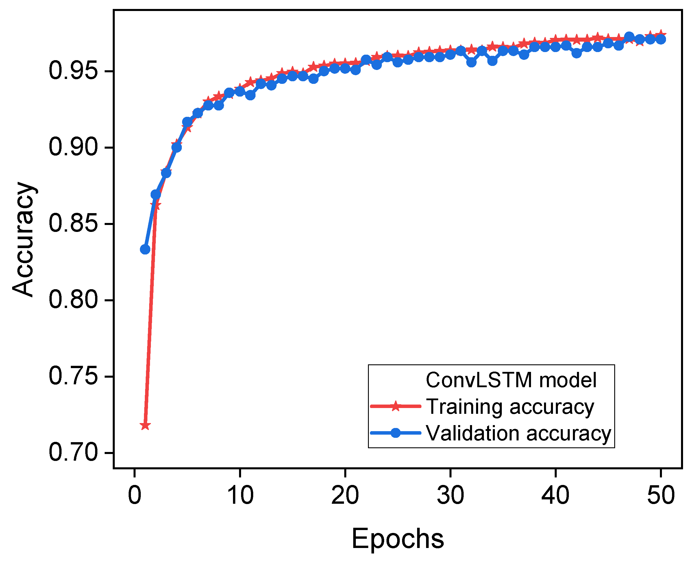
Figure 6 shows how well the ConvLSTM model predicted the system’s voltage stability during both the training and testing phases. This figure illustrates the notable precision of the ConvLSTM classifier, which achieved a commendable level of 0.9765 (97.65%). Initially, it is conceivable that the observer may not readily discern the remarkable patterns and correlations that exist between the input variables and the desired output.
However, with time, these patterns and correlations are likely to manifest themselves in a discernible manner. The ConvLSTM model demonstrates superior performance in strengthening its prediction skills by integrating information from previous time steps.
Furthermore, this feature allows the model to effectively capture and incorporate long-term dependencies, leading to the creation of predictions that are much more accurate and precise. However, a high accuracy value of 0.9765 may indicate the presence of overfitting when the model has potentially memorized the training data rather than effectively generalizing it to new, unseen data. The evaluation of the model in an independent test set is of the utmost importance to validating its generalizability. To address the difficulties related to overfitting, it is worth considering the utilization of regularization techniques such as dropout or weight decline. Figure 7 shows the loss curves of the ConvLSTM model during both the training and validation stages in the voltage stability data set. The proposed ConvLSTM algorithm is used to analyze the voltage stability data set, and its confusion matrix is shown in Figure 8.
However, with time, these patterns and correlations are likely to manifest themselves in a discernible manner. The ConvLSTM model demonstrates superior performance in strengthening its prediction skills by integrating information from previous time steps. The CNN model demonstrated a notable accuracy of 0.863 in its ability to predict voltage stability, as visually depicted in Figure 9.
The study presented here demonstrates the effective application of CNN models in classifying tabular data, despite their widespread use in image identification and processing tasks. In this situation, it is probable that the CNN model uses the inherent spatial correlations present in the input information. This enabled the model to effectively identify and extract significant patterns and features, resulting in a substantial improvement in its accuracy.
The convolutional layers played a pivotal role in the extraction of pertinent information by the application of filters or kernels to localized portions of the input. Nonlinear activation functions, such as Rectified Linear Units (ReLUs), are employed to inject nonlinearity into the models, hence augmenting their capabilities. The research study used a one-dimensional convolutional neural network (1DCNN) to make predictions regarding voltage stability. This was achieved by employing a particular data set that was specifically chosen for this purpose. Figure 10 illustrates the loss curves related to the CNN model. The findings suggest that the model exhibited a strong performance, as evidenced by an aggregate loss of 0.0962 and a training set accuracy of 0.8694.
In the validation set, the model achieved a recall value of 0.8908 and an accuracy score of 0.8694. Furthermore, the use of pooling layers effectively decreases the output dimensions, resulting in a reduction in parameters and serving as a preventive measure against overfitting. Ultimately, the convolutional and pooling outputs were processed by fully connected layers to provide predictions. Figure 11 presents a graphical representation of the confusion matrix. The results of this study emphasize the significant capabilities of the CNN model in correctly predicting voltage stability using a specific data set. The ability of the model to accurately predict outcomes in the validation set demonstrates its reliability and its ability to make accurate predictions for new, unseen data.
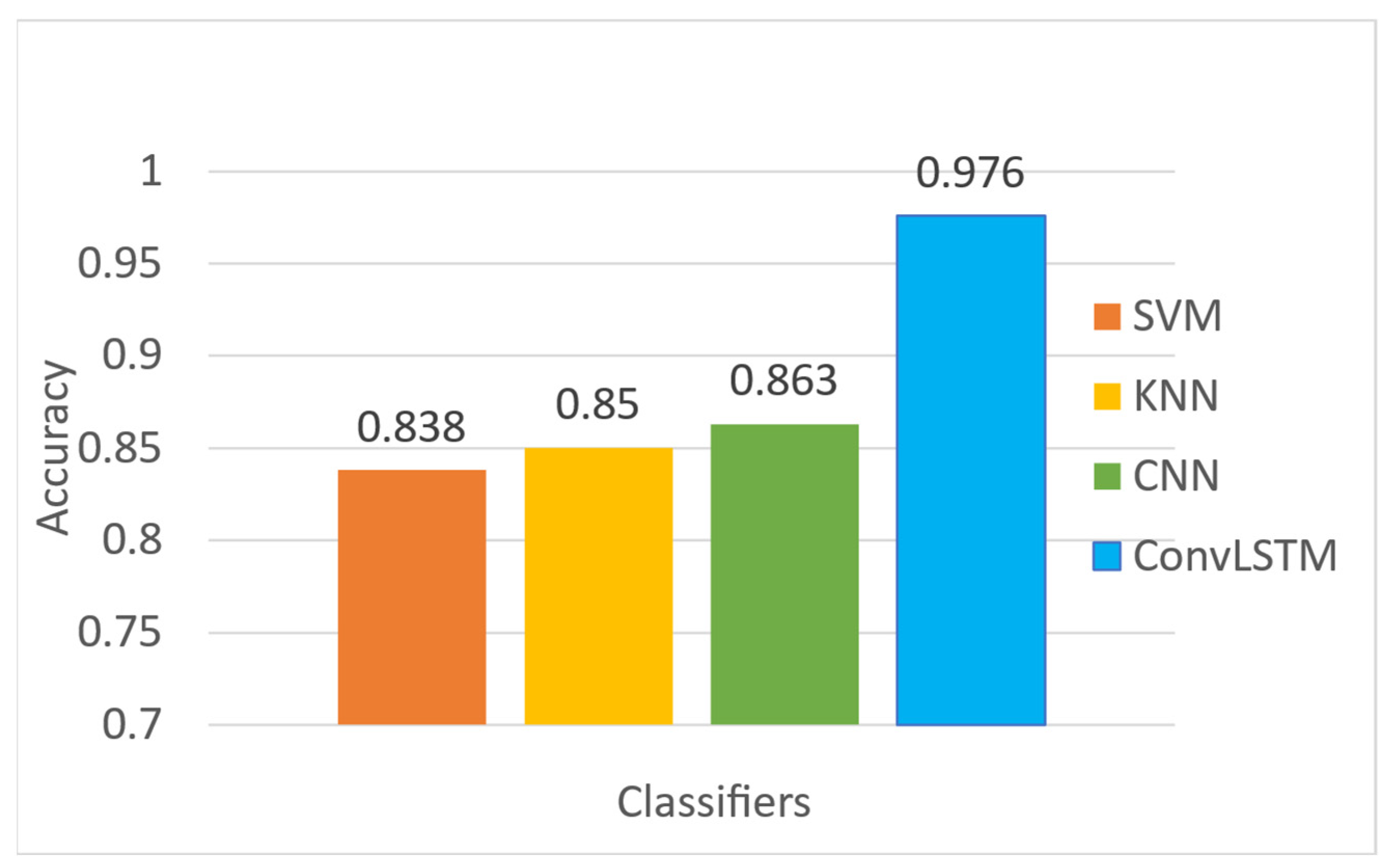
Figure 12 presents a comparison of the accuracy levels between the above ML and DL models used to predict the voltage stability of the IEEE 14-bus system. The data in this figure clearly indicate that the ConvLSTM classifier achieved the highest level of accuracy. In contrast, the SVM model exhibited the lowest performance, indicating its comparatively weaker performance in this study.
4. Conclusions and Future Research
In this study, many ML and DL algorithms have been used to predict the voltage stability of the IEEE 14-bus power system. In particular, the SVM model with a linear kernel showed a high degree of accuracy, especially with a regularization value C of 2. Meanwhile, the KNN method showed moderate but meaningful precision, with an optimal accuracy attained at a k value of 7. It used multiple distance measures in its calculations, which may explain its relatively high performance. The findings collected provide convincing proof that the suggested ConvLSTM model achieved a high accuracy of 97.65%. Furthermore, the ConvLSTM model surpasses the rest of the models, including the SVM, KNN, and CNN models, when examining their forecast accuracy for voltage stability. To improve the forecast ability of the ConvLSTM model for voltage stability in electric power systems, researchers could create an adaptive version of the ConvLSTM model in a short time by adjusting various configuration settings. This improved version has the ability to work well in microgrids within grid-off (isolated) mode and will apply to power grids with a larger number of buses for better voltage stability. This broader use and increased effectiveness have the potential to greatly enhance the stability of the voltage in a variety of contexts.
Author Contributions
Conceptualization, M.J.A.; Methodology, M.J.A. and M.A.; Software, M.J.A. and T.X.N.; Formal analysis, M.J.A. and M.A.; Investigation, T.X.N.; Resources, M.J.A.; Data curation, M.J.A. and M.A.; Writing—original draft, M.J.A.; Writing—review & editing, T.X.N.; Visualization, R.L.; Supervision, R.L.; Project administration, R.L.; Funding acquisition, R.L. All authors have read and agreed to the published version of the manuscript.
Funding
This research received no external funding.
Data Availability Statement
The original contributions presented in the study are included in the article, further inquiries can be directed to the corresponding authors.
Conflicts of Interest
The authors declare no conflict of interest.
References
- Lee, S.W.; Kim, H.Y. Stock market forecasting with super-high-dimensional time series data using ConvLSTM, trend sampling, and specialized data enhancement. Expert Syst. Appl. 2020, 161, 113704. [Google Scholar] [CrossRef]
- Sharma, G.; Singh, A.; Jain, S. A hybrid deep neural network approach to estimate reference evapotranspiration using limited climate data. Neural Comput. Appl. 2022, 34, 4013–4032. [Google Scholar] [CrossRef]
- Andersson, G.; Donalek, P.; Farmer, R.; Hatziargyriou, N.; Kamwa, I.; Kundur, P.; Martins, N.; Paserba, J.; Pourbeik, P.; Sanchez-Gasca, J.; et al. Causes of the 2003 major grid blackouts in North America and Europe and recommended means to improve system dynamic performance. IEEE Trans. Power Syst. 2005, 20, 1922–1928. [Google Scholar] [CrossRef]
- Glavic, M.; Van Cutsem, T. Wide-area detection of voltage instability from synchronized phasor measurements. Part I: Principle. IEEE Trans. Power Syst. 2009, 24, 1408–1416. [Google Scholar] [CrossRef]
- Shekari, T.; Gholami, A.; Aminifar, F.; Sanaye-Pasand, M. An adaptive wide-area load shedding scheme incorporating power system real-time limitations. IEEE Syst. J. 2016, 12, 759–767. [Google Scholar] [CrossRef]
- Wang, Y.; Pordanjani, I.R.; Li, W.; Xu, W.; Chen, T.; Vaahedi, E.; Gurney, J. Voltage stability monitoring based on the concept of coupled single-port circuit. IEEE Trans. Power Syst. 2011, 26, 2154–2163. [Google Scholar] [CrossRef]
- Chen, X.; Xie, X.; Teng, D. Short-term traffic flow prediction based on ConvLSTM model. In Proceedings of the 2020 IEEE 5th Information Technology and Mechatronics Engineering Conference (ITOEC), Chongqing, China, 12–14 June 2020; pp. 846–850. [Google Scholar] [CrossRef]
- Lin, Z.; Li, M.; Zheng, Z.; Cheng, Y.; Yuan, C. Self-attention convlstm for spatiotemporal prediction. In Proceedings of the AAAI Conference on Artificial Intelligence, New York, NY, USA, 7–12 February 2020; pp. 11531–11538. [Google Scholar] [CrossRef]
- Kundur, P. Power System Stability and Control, 1st ed.; McGraw-Hill Education: New York, NY, USA, 1994. [Google Scholar]
- Abbass, M.J.; Lis, R.; Mushtaq, Z. Artificial Neural Network (ANN)-Based Voltage Stability Prediction of Test Microgrid Grid. IEEE Access 2023, 11, 58994–59001. [Google Scholar] [CrossRef]
- Balu, C.; Maratukulam, D. Power System Voltage Stability; McGraw-Hill Education: New York, NY, USA, 1994. [Google Scholar]
- Fekri, M.N.; Grolinger, K.; Mir, S. Distributed load forecasting using smart meter data: Federated learning with Recurrent Neural Networks. Int. J. Electr. Power Energy Syst. 2022, 137, 107669. [Google Scholar] [CrossRef]
- Xiao, X.; Mo, H.; Zhang, Y.; Shan, G. Meta-ANN–A dynamic artificial neural network refined by meta-learning for Short-Term Load Forecasting. Energy 2022, 246, 123418. [Google Scholar] [CrossRef]
- Tang, X.; Chen, H.; Xiang, W.; Yang, J.; Zou, M. Short-term load forecasting using channel and temporal attention based temporal convolutional network. Electr. Power Syst. Res. 2022, 205, 107761. [Google Scholar] [CrossRef]
- Mohammadi, E.; Alizadeh, M.; Asgarimoghaddam, M.; Wang, X.; Simões, M.G. A review on application of artificial intelligence techniques in microgrids. IEEE J. Emerg. Sel. Top. Ind. Electron. 2022, 3, 878–890. [Google Scholar] [CrossRef]
- Shakerighadi, B.; Aminifar, F.; Afsharnia, S. Power systems wide-area voltage stability assessment considering dissimilar load variations and credible contingencies. J. Mod. Power Syst. Clean Energy 2019, 7, 78–87. [Google Scholar] [CrossRef]
- Venkatesan, R.; Li, B. Convolutional Neural Networks in Visual Computing: A Concise Guide; CRC Press: Boca Raton, FL, USA, 2017. [Google Scholar]
- Singh, P. Fundamentals and Methods of Machine and Deep Learning: Algorithms, Tools, and Applications; John Wiley & Sons: Hoboken, NJ, USA, 2022. [Google Scholar]
- Cortes, C.; Vapnik, V. Support-vector networks. Mach. Learn. 1995, 20, 273–297. [Google Scholar] [CrossRef]
- Khater, S.; Hadhoud, M.; Fayek, M.B. A novel human activity recognition architecture: Using residual inception ConvLSTM layer. J. Eng. Appl. Sci. 2022, 69, 45. [Google Scholar] [CrossRef]
- Agga, A.; Abbou, A.; Labbadi, M.; El Houm, Y. Short-term self consumption PV plant power production forecasts based on hybrid CNN-LSTM, ConvLSTM models. Renew. Energy 2021, 177, 101–112. [Google Scholar] [CrossRef]
- Moishin, M.; Deo, R.C.; Prasad, R.; Raj, N.; Abdulla, S. Designing deep-based learning flood forecast model with ConvLSTM hybrid algorithm. IEEE Access 2021, 9, 50982–50993. [Google Scholar] [CrossRef]
- Bendaouia, A.; Qassimi, S.; Boussetta, A.; Benzakour, I.; Amar, O.; Hasidi, O. Artificial intelligence for enhanced flotation monitoring in the mining industry: A ConvLSTM-based approach. Comput. Chem. Eng. 2024, 180, 108476. [Google Scholar] [CrossRef]
- Nazari-Heris, M.; Asadi, S.; Mohammadi-Ivatloo, B.; Abdar, M.; Jebelli, H.; Sadat-Mohammadi, M. Application of Machine Learning and Deep Learning Methods to Power System Problems; Springer: Berlin/Heidelberg, Germany, 2021. [Google Scholar]
Figure 1.
Architecture of modern power grids, including traditional generation and DRESs [10].
Figure 1.
Architecture of modern power grids, including traditional generation and DRESs [10].

Figure 2.
Typical electrical power system.

Figure 3.
Power voltage curve (P-V) [16].
Figure 3.
Power voltage curve (P-V) [16].

Figure 4.
Structure of the deep learning ConvLSTM model.

Figure 5.
Deep learning-based architecture of modern power systems [10].
Figure 5.
Deep learning-based architecture of modern power systems [10].

Figure 6.
Training and validation accuracy of the ConvLSTM model for prediction of the voltage stability of the IEEE 14-bus system.
Figure 6.
Training and validation accuracy of the ConvLSTM model for prediction of the voltage stability of the IEEE 14-bus system.

Figure 7.
Predicting the voltage stability of the proposed IEEE 14-bus system using the ConvLSTM model resulted in a loss during training and validation.
Figure 7.
Predicting the voltage stability of the proposed IEEE 14-bus system using the ConvLSTM model resulted in a loss during training and validation.

Figure 8.
The confusion matrix of the ConvLSTM model predicts the voltage stability of the IEEE 14-bus power grid.
Figure 8.
The confusion matrix of the ConvLSTM model predicts the voltage stability of the IEEE 14-bus power grid.

Figure 9.
The accuracy of the CNN model in predicting voltage stability of the IEEE 14-bus power grid through training and validation.
Figure 9.
The accuracy of the CNN model in predicting voltage stability of the IEEE 14-bus power grid through training and validation.

Figure 10.
Loss of training and validation of the CNN model for predicting the voltage stability of the IEEE 14-bus power grid.
Figure 10.
Loss of training and validation of the CNN model for predicting the voltage stability of the IEEE 14-bus power grid.

Figure 11.
Confusion matrix for 1DCNN applied to the voltage stability data set.

Figure 12.
Comparison of the accuracy of the models in predicting voltage stability.


Table 1.
Summary of the CNN model.
| Layer (Type) | Output Shape | Parameter |
|---|---|---|
| conv1d_8 (Conv1D) | (None, 7, 32) | 256 |
| conv1d_9 (Conv1D) | (None, 3, 48) | 7728 |
| conv1d_10 (Conv1D) | (None, 1, 48) | 6960 |
| flatten_1 (flatten) | (None, 48) | 0 |
| dense_5 (dense) | (None, 64) | 3136 |
| dropout_1 (dropout) | (None, 64) | 0 |
| dense_6 (Dense) | (None, 1) | 65 |
| Total parameters: 18,145 Trainable parameters: 18,145 Non-trainable parameters: 0 | ||
Table 2.
Classifiers of the KNN and SVM models.
| Classifier | Stemmer | |||
|---|---|---|---|---|
| Porter | Lovin | Wordnet | ||
| KNN | Euclidean | 89.9% | 92.8% | 95.7% |
| Cosine | 90.9% | 93.8% | 95.4% | |
| Correlation | 92.9% | 94.8% | 96.0% | |
| SVM | RBF | 77.9% | 92.8% | 79.7% |
| Linear | 80.9% | 93.8% | 80.4% | |
| Sigmoid | 81.6% | 94.8% | 82.0% | |
Disclaimer/Publisher’s Note: The statements, opinions and data contained in all publications are solely those of the individual author(s) and contributor(s) and not of MDPI and/or the editor(s). MDPI and/or the editor(s) disclaim responsibility for any injury to people or property resulting from any ideas, methods, instructions or products referred to in the content. |
© 2024 by the authors. Licensee MDPI, Basel, Switzerland. This article is an open access article distributed under the terms and conditions of the Creative Commons Attribution (CC BY) license (https://creativecommons.org/licenses/by/4.0/).
Share and Cite
MDPI and ACS Style
Abbass, M.J.; Lis, R.; Awais, M.; Nguyen, T.X. Convolutional Long Short-Term Memory (ConvLSTM)-Based Prediction of Voltage Stability in a Microgrid. Energies 2024, 17, 1999. https://doi.org/10.3390/en17091999
AMA Style
Abbass MJ, Lis R, Awais M, Nguyen TX. Convolutional Long Short-Term Memory (ConvLSTM)-Based Prediction of Voltage Stability in a Microgrid. Energies. 2024; 17(9):1999. https://doi.org/10.3390/en17091999
Chicago/Turabian StyleAbbass, Muhammad Jamshed, Robert Lis, Muhammad Awais, and Tham X. Nguyen. 2024. "Convolutional Long Short-Term Memory (ConvLSTM)-Based Prediction of Voltage Stability in a Microgrid" Energies 17, no. 9: 1999. https://doi.org/10.3390/en17091999
Note that from the first issue of 2016, this journal uses article numbers instead of page numbers. See further details here.