A Systematic Investigation into the Optimization of Reactive Power in Distribution Networks Using the Improved Sparrow Search Algorithm–Particle Swarm Optimization Algorithm

Abstract

With the expansion of the scale of electric power, high-quality electrical energy remains a crucial aspect of power system management and operation. The generation of reactive power is the primary cause of the decline in electrical energy quality. Therefore, optimization of reactive power in the power system becomes particularly important. The primary objective of this article is to create a multi-objective reactive power optimization (MORPO) model for distribution networks. The model aims to minimize reactive power loss, reduce the overall compensation required for reactive power devices, and minimize the total sum of node voltage deviations. To tackle the MORPO problems for distribution networks, the improved sparrow search algorithm–particle swarm optimization (ISSA-PSO) algorithm is proposed. Specifically, two improvements are proposed in this paper. The first is to introduce a chaotic mapping mechanism to enhance the diversity of the population during initialization. The second is to introduce a three-stage differential evolution mechanism to improve the global exploration capability of the algorithm. The proposed algorithm is tested on the IEEE 33-node system and the practical 22-node system. The results indicate a reduction of 32.71% in network losses for the IEEE 33-node system after optimization, and the average voltage of the circuit increases from 0.9485 p.u. to 0.9748 p.u. At the same time, optimization results in a reduction of 44.07% in network losses for the practical 22-node system, and the average voltage of the circuit increases from 0.9838 p.u. to 0.9921 p.u. Therefore, the proposed method exhibits better performance for reducing network losses and enhancing voltage levels.

1. Introduction

The field of reactive power optimization in modern power grids is constantly evolving and improving as technologies progressively shift towards intelligence, real-time operation, and coordination to address the complexity and variability of power system operation. This enhances the operational efficiency, economic viability, and reliability of the grid. Reasonable strategies for reactive power control and allocation can reduce energy consumption and operational costs in the power grid, ultimately enhancing the stability and economic efficiency of the power system. Conversely, the insufficiency of reactive power and improper distribution in the power distribution system may result in increased line losses and voltage fluctuations. However, the modern reactive power optimization (RPO) field also faces various issues and challenges, including those presented by demand growth, the limitations of traditional reactive power compensation devices, and the intricate grid topology, among other challenges [1].

The RPO of distribution networks in the power system is a subproblem of the optimal power flow problem. RPO can be achieved by manipulating the reactive power for the power system, thereby enhancing the efficiency of the power system [2]. The primary objective of RPO is to achieve optimal operating conditions while satisfying the given constraints by harmonizing and optimizing control variables such as generator voltage values and transformer voltage ratios, which aim to reduce network losses and improve voltage levels [3,4].

In general, RPO models presented a single-objective function, such as minimizing reactive power losses or optimizing reactive power distribution. In recent years, with the increasing demands for grid stability and reliability, researchers have begun to explore multi-objective optimization problems. In addition to minimizing reactive power losses, reactive power optimization models also considered other objective functions, such as improving voltage stability, power factor, and reactive power balance. Therefore, the optimization problem has evolved from a single-objective RPO problem to a multi-objective reactive power optimization (MORPO) problem [5,6]. The MORPO problem is essentially a nonlinear optimization problem with multiple constraints, variables, and objectives [7,8].

To address this issue, numerous scholars have proposed various solutions, which are mainly divided into two categories: classical optimization techniques and artificial intelligence optimization technologies. The classical optimization techniques consist of gradient methods [9], interior point methods [10], linear programming [11], and nonlinear programming methods [12]. To solve multi-objective problems, the traditional approaches generally transformed the MORPO problem into a single-objective optimization problem by using weighted methods [13], ε-constraint methods [14], and fuzzy decision-making methods [15]. However, there are inherent drawbacks to traditional methods, such as computational complexity, limited flexibility, and the inability to solve constrained problems involving nonlinear and discontinuous functions. Therefore, artificial intelligence optimization algorithms have gradually been employed to tackle multi-objective optimization problems. Recently, the MORPO problem has been successfully addressed through the implementation of metaheuristic optimization methodologies, with examples such as particle swarm optimization (PSO) [16,17], the sine cosine algorithm (SCA) [18], the sparrow search algorithm (SSA) [19], the imperialist competitive algorithm (ICA) [20], the cuckoo search algorithm (CSA) [21,22], the genetic algorithm (GA) [23], the beetle antenna search (BAS) algorithm [24], the NSGA-II algorithm [25], the grey wolf optimization (GWO) algorithm [26,27], the bacterial foraging optimization (BFO) algorithm [28], etc.

The PSO algorithm, known for its low memory requirements and fast convergence, has been widely adopted in the field of MORPO due to its advantages [29]. In reference [30], an improved RPO algorithm was proposed by considering the minimization of power loss as the primary objective function, which was achieved by enhancing the strategy of inertia weight and the acceleration coefficients. In reference [31], the L-index was incorporated to enhance the stability of static voltage in electrical power systems. Confronted with intricate multi-objective dilemmas, such as minimizing power loss and L-index, the implementation of a crossover operator was introduced to augment the diversity of PSO. Additionally, a chaotic sequence based on logical mapping was utilized in PSO instead of a random sequence to enhance its global search capability and exploitation ability. In reference [32], the potential effects of integrating distributed generation (DG) into the power distribution network were discussed. An improved second-order oscillatory PSO algorithm was presented to enhance the efficiency and convergence properties of multi-objectives. It should be noted that multiple iterations are required to converge for the PSO algorithm. Consequently, this can lead to the PSO algorithm easily becoming trapped in a local optimum solution [33].

The SSA is a novel nature-inspired algorithm that draws inspiration from the behavior of sparrows [34]. It has gained widespread discussion among scholars and is currently under active research. In reference [35], a multi-objective optimization model was established including investment cost, environmental sustainability, and power supply quality as the objective functions. Subsequently, the Levy flight strategy was incorporated into the SSA to enhance the ability of the multi-objective sparrow search algorithm to escape local optima. In reference [36], a chaotic sparrow searches algorithm (CLSSA) based on the logarithmic spiral strategy and the adaptive step size strategy was proposed. The experimental findings demonstrate the commendable practicality of the proposed approach in addressing engineering quandaries. In reference [37], this article aims to integrate an improved point selection strategy with the SSA. The issue of convergence degradation in solving high-dimensional multi-objective optimization problems has been resolved and the performance of the algorithm is improving. Based on the above research, it can be observed that despite the excellent performance of the SSA in optimization problems, it has some inherent drawbacks, such as slow convergence speed and the possibility of becoming trapped in local optima.

According to the aforementioned research, this paper proposes a method for MORPO in distribution networks using the improved sparrow search algorithm–particle swarm optimization (ISSA-PSO) algorithm. The specific findings and contributions of the paper can be summarized as follows:

(1) This paper establishes a MORPO model, where the objective function consists of minimizing active power loss, minimizing total compensation of reactive power compensation devices, and minimizing the sum of node voltage deviations.

(2) Inspired by the aforementioned research, this paper presents the ISSA-PSO algorithm to address the low convergence accuracy in PSO while incorporating the strong global search capability and efficiency of SSA. This algorithm incorporates two notable enhancements: The first enhancement introduces the incorporation of a tent chaotic mapping mechanism to initialize the population, aiming to enhance its diversity. The second enhancement introduces a three-stage differential evolution mechanism to enhance the algorithm’s global exploration capability.

(3) The effectiveness of the ISSA-PSO algorithm is proved by simulation using the IEEE 33-node system and the practical 22-node system. Compared with the SSA, PSO algorithm, and SSA-PSO algorithm, the proposed strategy has better performance in terms of tracking speed, accuracy, and dependability.

2. MORPO Model

The essence of MORPO in distribution networks is essentially the resolution of a nonlinear problem that contains both equality and inequality constraints. By incorporating the actual characteristics of the power system into the reactive power problem and considering given parameters such as impedance values and load conditions of the distribution lines, the control variables are optimized to satisfy the constraints set for the objective function. Consequently, the distribution network achieves an optimal operational state through MORPO. The mathematical model is defined as follows:

$$\left\{\begin{array}{c}minf(u,x)\\ s.t.g(u,x)=0\\ h(u,x)\le 0\end{array}\right.,$$

(1)

where $minf(u,x)$ is the objective function; $g(u,x)=0$ is the equality constraint; and $h(u,x)\le 0$ represents the inequality constraint.

2.1. Selecting the Objective Function

(1) From an economic perspective, the minimization of active power losses in the distribution network system is considered as the first objective function. The expression can be formulated as follows:

$$min{P}_{loss}=min{\sum }_{j\in i}^{i\in n}{G}_{ij}·\left[U_i^2+U_j^2-2U_i{U}_j·\cos {(\theta }_i-{\theta }_j)\right],$$

(2)

where $P_{loss}$ indicates the active power loss in the power grid; n is the number of branches; G is line conductivity; and U and $\theta$ are the amplitude and phase angle of voltage.

(2) The second objective function aims to minimize the total amount of compensation for the installed compensating devices in the power system; the expression is as follows:

$$minf=min{\sum }_{i=1}^{N_c}({\alpha }_i·Q_{Ci})+\beta ·P_{loss},$$

(3)

where ${\alpha }_i$ is the power factor correction coefficient for the annual reactive power consumption of node i; $N_c$ is the selected number of compensation nodes; $Q_{Ci}$ is the compensation amount under node i; and $\beta$ is the cost factor of network loss with power generation.

(3) The third objective function is to minimize the total sum of nodal voltage deviations in the power system; the expression is as follows:

$$dU=\left|\sqrt{{[U_{j\left(x\right)}-∆U_{ij\left(x\right)}]}^2+{\left[\delta U_{ij\left(x\right)}\right]}^2}-U_N\right|/U_N,$$

(4)

where N is the total number of nodes; $U_N$ is the rated voltage; $∆U_{ij}$ is the longitudinal component of voltage drop; and $\delta U_{ij}$ is the lateral component of voltage drop.

The penalty functions are incorporated into the establishment of the MORPO model, transforming the multi-objective problem into a single-objective one, ensuring a more accurate optimization of the model. The explanation of a penalty function is as follows. When all inequality constraints are satisfied, the penalty term equals zero. However, as soon as any inequality constraint is not satisfied, the corresponding penalty term is generated, and the larger the deviation, the greater the value of the penalty term. This effectively increases the objective function, serving as a punishment for not meeting the constraints. When the penalty factor is sufficiently large, the optimization process can only minimize the penalty function by gradually approaching zero. This compels the previously violated variables or functions to converge or return within the specified limits of their constraints. Utilizing mathematical models that integrate systemic economic benefits and security, we can formulate a precise expression:

$$F_{min}=P_{loss}+{\delta }_V·{\sum }_m{(\frac{∆V_i}{V_{imax}-V_{imin}})}^2+{\delta }_Q·{\sum }_n{(\frac{∆Q_{Gi}}{Q_{Gimax}-Q_{Gimin}})}^2,$$

(5)

where the second item pertains to the penalty for excessive voltage at the PQ node; the third item pertains to the penalties for exceeding the limits of reactive power compensation; m is the set of nodes for all generators in this system; ${\delta }_V$ is the penalty factor for PQ node voltage violation; $∆V_i$ is the deviation of the voltage at the i node; $Q_{Gi}$ is compensation amount under node i; and ${\delta }_Q$ is the penalty factor for overcompensation of reactive power.

The specified conditions for punitive measures are as follows:

$$∆V_i=\left\{\begin{array}{c}{V}_{imin}-V_i\hspace{1em}(V_i<V_{imin})\\ \hspace{1em}0\hspace{1em}(V_{imin}<V_i<V_{imax})\\ V_i-V_{imax\hspace{1em}}(V_{imax}<V_i)\end{array}\right.,$$

(6)

$$∆Q_{Gi}=\left\{\begin{array}{c}{Q}_{Gimin}-Q_{Gi}\hspace{1em}(Q_{Gi}<Q_{Gimin})\\ 0\hspace{1em}(Q_{Gimin}<Q_{Gi}<Q_{Gimax})\\ Q_{Gi}-Q_{Gimax}\hspace{1em}(Q_{Gimax}<Q_{Gi})\end{array}\right.,$$

(7)

where $V_{imax}$ and $V_{imin}$ are the upper and lower bounds of nodal voltage; and $Q_{Gimax}$ and $Q_{Gimin}$ are the upper and lower reactive power compensation capacity.

2.2. Constraint Condition

(1)

Equality constraint condition

The formulation of equation constraints is intended to ensure the conservation of active and reactive power within the system. To ensure the secure and stable operation of the power system, certain measures must be implemented. The equation of constraint is as follows:

$$\left\{\begin{array}{c}{P}_i=P_{Gi}-P_{Li}=U_i\sum _{j=1}^n{U}_j·(G_{ij}\cos {\delta }_{ij}+B_{ij}\sin {\delta }_{ij})\\ Q_i=Q_{Gi}-Q_{Li}=U_i\sum _{j=1}^n{U}_j·(G_{ij}\sin {\delta }_{\mathit{ij}}+B_{ij}\cos {\delta }_{ij})\end{array}\right.,$$

(8)

where P and Q are active power and reactive power; $\delta$ is the phase angle difference; $P_{Gi} \mathrm{and} Q_{Gi}$ are the active power output and reactive power output of the generator node; and $P_{Li} \mathrm{a}\mathrm{n}\mathrm{d} Q_{Li}$ are the active load, reactive load, and reactive compensation capacity of nodes.

(2)

Inequality constraint condition

In the process of optimization and adjustment, the voltage at the generator’s nodes $V_G$, the compensating capacity of the parallel capacitors $Q_C$, and the tap changer T of the transformer are regarded as control variables, while the reactive power output of the node voltage is judged as the changeable state.

The inequality constraints for controlling variables are as follows:

$$\left\{\begin{array}{c}{V}_{Gmin}\le V_G\le V_{Gmax}\\ T_{min}\le T\le T_{max}\\ Q_{Cmin}\le Q_C\le Q_{Cmax}\end{array}\right..$$

(9)

The inequality constraint conditions of the state variables are as follows:

$$\left\{\begin{array}{c}{Q}_{Gmin}\le Q_G\le Q_{Gmax}\\ V_{dmin}\le V_d\le V_{dmax}\end{array}\right.,$$

(10)

where $V_G$ is the voltage at the terminals of the generator and $V_{Gmin}$, $V_{Gmax}$ are the corresponding upper and lower thresholds; T, $T_{min}, \mathrm{and} T_{max}$ are the relative positioning and upper/lower limit values of the tap changer systems in the transformers; $Q_G$ is the reactive power output of a generator and $Q_{Gmin},Q_{Gmax}$ are the upper and lower limits; and $Q_C$ is the voltage at the node and $Q_{Cmin}$, $Q_{Cmax}$ are the corresponding upper and lower limits.

3. The Improved Particle Swarm Optimization–Sparrow Search Algorithm

3.1. Sparrow Search Algorithm

The SSA is an intelligent algorithm inspired by the hunting behavior of sparrows. It possesses excellent capabilities for local exploration and global optimization. The process of sparrow predation can be divided into two primary roles: the discoverer and the follower. The discoverer, characterized by a higher energy level, provides the direction to the food source for the population. The remaining individuals serve as followers who trail the discoverer in search of food, and they may even become involved in disputes over resources. Moreover, a certain proportion of sparrows possess the ability of vigilant surveillance, allowing them to evade potential predators.

The discoverer undertakes the task of foraging for sustenance and guiding the collective migration of the entire population. Therefore, the discoverer may explore sustenance in a more extensive realm than the one inhabited by the joiner. The formula for updating the position of the discoverer is as follows:

$$X_{i,j}^{t+1}=\left\{\begin{array}{cc}{X}_{i,j}^t·\exp \left(\frac{-i}{\alpha ·{\mathrm{i}\mathrm{t}\mathrm{e}\mathrm{r}}_{\mathrm{m}\mathrm{a}\mathrm{x}}}\right)& if R_2<ST\\ X_{i,j}^t+Q·L& if R_2\ge ST\end{array}\right.,$$

(11)

where $X_{i,j}^t$ is the i-th individual in the j-th dimension value following t iterations; $R_2$ is the early warning value; $\alpha$ represents random numbers, $\alpha \in$ (0,1]; ST is the safety threshold, $ST\in$ (0.5,1]; Q represents random numbers obeying the normal distribution; and L is a matrix consisting of elements that are all 1.

If $R_2<ST$, this means the absence of predators, prompting the observer to engage in an extensive exploration mode. Otherwise, if $R_2\ge ST$, all the sparrows must expeditiously migrate to alternative safe havens upon the discovery of predators in their vicinity.

Once the sparrows perceive that the discoverer has identified a region with splendid nourishment, they will relinquish their current location and migrate to the discoverer’s position to contend for the food resources. In the event of their successful occupation of the designated vantage point, the discoverer shall be rewarded with nourishment. Otherwise, they shall persist in adhering to the established regulations. The formula for the position of the follower update is as follows:

$$X_{i,j}^{t+1}=\left\{\begin{array}{cc}Q·(\frac{X_{worst}^t-X_{i,j}^t}{i^2})& if i>n/2\\ X_P^{t+1}+\left|X_{i,j}^t-X_P^{t+1}\right|·A^{+}·L& if i\le n/2\end{array}\right.,$$

(12)

where $X_P$ is the optimal position occupied by the discoverer, and $X_{worst}$ is the current worst-case global position.

According to the aforementioned formula, the mathematical model can be expressed as follows:

$$X_{i,j}^{t+1}=\left\{\begin{array}{cc}{X}_{best}^t+\beta ·\left|X_{i,j}^t-X_{best}^t\right|& if f_i>f_g\\ X_{i,j}^t+K·(\frac{\left|X_{i,j}^t-X_{worst}^t\right|}{{(f}_i-f_w)+\epsilon })& if f_i=f_g\end{array}\right.,$$

(13)

where $X_{best}$ is the current global optimal position; $\beta$ represents the step size control parameters, conforming to a Gaussian distribution of random numbers with a mean of 1 and a variance of 1; $f_i$ is the present fitness value of the sparrows; $f_g$ is the current global best fitness value; $f_w$ is the present minimum fitness value in the global range; and $\epsilon$ is the minimum constant selected to avoid errors in the division by zero.

3.2. Particle Swarm Optimization

PSO is an algorithm of collective intelligence, conceived in the spirit of bird foraging behavior. This algorithm solves optimization problems by emulating the foraging behavior of avian species traversing multidimensional search spaces. In the PSO algorithm, the solution to a problem is represented as the position of a particle, with each particle representing a candidate solution in the problem space. The Formulas (14) and (15) express the updates for velocity and position in the PSO algorithm, respectively.

$$v_i^{t+1}=\omega ·v_i^t+c_1·\mathrm{r}\mathrm{a}\mathrm{n}\mathrm{d}\mathrm{i}(p_{best}-x_i^t)+c_2·\mathrm{r}\mathrm{a}\mathrm{n}\mathrm{d}\mathrm{i}(g_{best}-x_i^t),$$

(14)

$$x_i^{t+1}=x_i^t+v_i^{t+1},$$

(15)

where $v_i^t$ is the velocities of the i-th particle at the t and t + 1 iterations; $c_1$ and $c_2$ are acceleration factors; $p_{best}$ and $g_{best}$ are the local and global optimal positions of particles; ${\mathrm{rand}}_1$ and ${\mathrm{rand}}_2$ are random numbers ranging from 0 to 1; and $\omega$ is the inertia weight.

The advantages of the PSO algorithm include ease of implementation, obviating the need to calculate gradient information, applicability to both continuous and discrete optimization problems, etc. However, the PSO algorithm has some certain drawbacks, such as its susceptibility to becoming trapped within local optima, its sensitivity to problem initialization, etc.

3.3. Sparrow Search Algorithm–Particle Swarm Optimization

In order to tackle the problem of limited local search capacity and insufficient search accuracy in PSO, the SSA is introduced. To tackle the problems of search stagnation and the challenge of breaking free from a limited search space, a subgroup of the PSO population known as sparrows is incorporated, which are further classified into discoverers, trackers, and sentinels.

The formula is then updated as follows:

$$v_{id}=\omega ·v_{id}+c_1·r_1\left(p_{id}-x_{id}\right)+c_2·r_2\left(p_{gd}-x_{gd}\right),$$

(16)

where $\omega$ is the weight coefficient, with an initial value of 0.5; $c_1$ and $c_2$ are the pursuit of knowledge, with an initial value of 0.1 and 0.5; $p_{id}$ is the individual optimal position; $p_{gd}$ is the global optimal position; and $r_1$ and $r_2$ are random numbers.

The formula for updating the position of each discoverer is defined as follows:

$$X_{i,j}^{t+1}=\left\{\begin{array}{ll}{X}_{i,j}^t·\exp (\frac{-i}{\alpha ·t_{max}})& if A>T_s\\ X_{i,j}^t+Q·L& if A\le T_s\end{array}\right.,$$

(17)

where $X_{i,j}^t$ is the coordinate information of sparrow i in dimension j in the t-th generation, where j = 2; $\alpha$ is a random number; A is an alert value, $A\in$ [0,1]; $T_s$ is the safety threshold, $T_s\in \left[0.5,0.7\right]$; and Q represents random numbers obeying the normal distribution.

When A < $T_s$, it indicates the absence of danger nearly, and the discoverer at this moment may engage in a search within a broader spatial range. When A ≥ $T_s$, the observer perceives danger, and some sparrows follow the discoverer’s actions as a follower. However, upon the discovery of food, these followers will approach and contend with the finder for sustenance. A small portion of the followers, due to insufficiency of sustenance, will fly to other areas to search for food, replenishing the necessary sustenance. The formula for updating is defined as follows:

$$X_{i,j}^t=\left\{\begin{array}{cc}\hspace{1em}\hspace{1em}Q·\exp (\frac{x{\omega }_{i,j}^t-x_{i,j}^t}{i^2})\hfill & if i>n/2\\ x{b}_{i,j}^t+\frac{1}{J}\left(\mathrm{rand}\right)\left\{-1,1\right\}·\left(\left|x{b}_{i,j}^t-b_{i,j}^t\right|\right)& if i\le n/2\end{array}\right.,$$

(18)

where N is the population, N = 100; $x{b}_{i,j}^t$ is the best currently discovered food source; and $x{\omega }_{i,j}^t$ is the worst current global food source.

The formula for updating the position of the observer is as follows:

$$X_{i,j}^{t+1}=\left\{\begin{array}{cc}x·b_{i,j}^t+\beta ·\left(x_{i,j}^t-x{b}_{i,j}^t\right)& f_i\ne f_g\\ x·b_{i,j}^t+K·(\frac{x_{i,j}^t-x{\omega }_{i,j}^t}{\left|f_i-f_g\right|+\epsilon })& f_i=f_g\end{array}\right.,$$

(19)

where $x{b}_{i,j}^t$ is the optimal food source discovered by the population of sparrows; $\beta$ is the step size adjustment factor; $\epsilon$ is a minuscule constant; K is a random number, $K\in \left[-1,1\right]$; $f_i$ is the present fitness value; and $f_g$ is the current global best fitness value.

The weighting factor adopts a sinusoidal variation; the weight factor of the algorithm is represented by the following equation:

$$\omega \left(k\right)=\frac{{\omega }_{max}-{\omega }_{min}}{k}·\sin (\pi \frac{k}{k_{max}})+\frac{{\omega }_{max}+{\omega }_{min}}{k},$$

(20)

where ${\omega }_{max}$ = 1, ${\omega }_{min}$ = 0.5; k represents iterations; $k_{max}$ is the maximum number of iterations; and $\omega$(k) is the inertia weight factor for the k-th iteration.

The flowchart of the SSA-PSO algorithm is shown in Figure 1 as follows.

3.4. The Improved SSA-PSO Algorithm

The SSA-PSO algorithm combines the advantages of both the SSA and the PSO algorithm, significantly improving the algorithm’s optimization accuracy and efficiency. However, The SSA-PSO algorithm still possesses untapped potential for optimization. Therefore, this paper undertakes further optimization based on SSA-PSO: the first improvement is the introduction of a chaotic mapping mechanism to enhance the diversity of the population during initialization, and the second is the introduction of a three-stage differential evolution mechanism to improve the global exploration capability of the algorithm.

• Tent chaotic map

A tent chaotic map is a piecewise linear one-dimensional map. Compared to the logistic function, it exhibits a uniform power spectral density, probability density, and ideal correlation characteristics, along with a faster iteration rate. The mathematical expression is as follows:

$$x_{n+1}=a-1-a·\left|x_n\right|,\hspace{1em}a\in \left(1,2\right)$$

(21)

When a ≤ 1, the tent chaotic map is in a stable state; when 1 < a < 2, the tent chaotic map is in a state of chaotic dynamics; when a = 2, the tent chaotic map is the core of tent mapping. The mathematical expression is as follows:

$$x_{k+1}=\left\{\begin{array}{cc}2x_k,& 0\le x_k\le 0.5\\ 2\left(1-x_k\right),& 0.5\le x_k\le 1\end{array}\right.$$

(22)

The tent chaotic map exhibits remarkable traversability, and the computation processing is suitable for a large magnitude of data sequences. However, the mapping of the tent function suffers from the drawback of having a small unstable period. Therefore, the following enhancements for the tent mapping are proposed.

$$x_{k+1}=\left\{\begin{array}{cc}2·\left(x_k+0.1·\mathrm{rand}(0,1)\right),& 0\le x_k\le 0.5\\ 2·\left(1-\left(x_k+0.1·\mathrm{rand}(0,1)\right)\right),& 0.5\le x_k\le 1\end{array}\right.$$

(23)

• The three-stage differential evolution mechanism (TSDE)

The TSDE is an evolutionary algorithm commonly used for solving optimization problems. It is an enhanced version of the differential evolution (DE) algorithm. The essence of TSDE lies in iteratively optimizing individuals to seek the optimal solution. In each generation, superior individuals are chosen and preserved by comparing the fitness of the parent population with that of the offspring population. Simultaneously, less adaptive individuals are replaced by newly generated individuals. For individuals with lower fitness, improvement can be achieved by adopting superior mutation and crossover strategies. Compared to traditional DE algorithms, TSDE incorporates a design consisting of three stages, which enhances the stability and convergence of the algorithm. Additionally, TSDE can be customized by employing different mutation and crossover operations tailored to the characteristics of specific problems. This adaptability and flexibility enable TSDE to effectively tackle diverse optimization problems. The three stages of TSDE are as follows:

Initialization phase: During this stage, the population needs to be initialized by generating a set of candidate solutions. Common methods for initialization include random generation, uniform distribution, or specific initialization based on the characteristics of the problem. The expression in the initialization phase is as follows:

$$x_i\left(t+1\right)=x_i\left(t\right)+C\cdot \left(x_i\left(t\right)-x_1\left(t\right)\right),\hspace{1em}i\in \left[2,\dots ,n\right],$$

(24)

where C represents consumer factors with Levy flight characteristics.

$$C=\frac{1}{2}·\frac{v_1}{\left|v_2\right|},$$

(25)

$$v_1~N\left(0,1\right),\hspace{1em}{v}_2~N\left(0,1\right),$$

(26)

where N (0, 1) is the probability density function of a normal distribution with mean 0 and standard deviation 1; and $v_1$ and $v_2$ are the standard normal distribution.

Mutation and crossover phase: During this phase, new individuals are generated by selecting parent individuals and performing mutation and crossover operations. Specifically, the mutation operation introduces small perturbations to the parent individuals to obtain new individuals, while the crossover operation combines the new individuals with the original individuals to produce offspring individuals. The expressions for the mutation and crossover phase are as follows:

$$\left\{\begin{array}{c}{x}_i\left(t+1\right)=x_i\left(t\right)+C\cdot \left(x_i\left(t\right)-x_j\left(t\right)\right),\hspace{1em}i\in \left[3,\dots ,n\right]\\ j=\mathrm{randi}(\left[2i-1\right])\end{array}\right.,$$

(27)

where $x_j\left(t\right)$ is the optimal individual from the t-th iteration.

Selection phase: During this phase, individuals with higher fitness from both the parent and offspring populations are chosen as parents for the next generation based on a predetermined strategy. The expression for the selection phase is as follows:

$$x_i\left(t+1\right)=x_i\left(t\right)+C\cdot \left(r_2\cdot \left(x_i\left(t\right)-x_1\left(t\right)\right)\right.+\left(1-r_2\right)\left(x_i\left(t\right)-x_j\left(t\right)\right),\hspace{1em}i=3,\dots ,n,$$

(28)

$$j=\mathrm{randi}(\left[2i-1\right]),$$

(29)

where $r_2$ is a random number, $r_2\in \left[0,1\right]$.

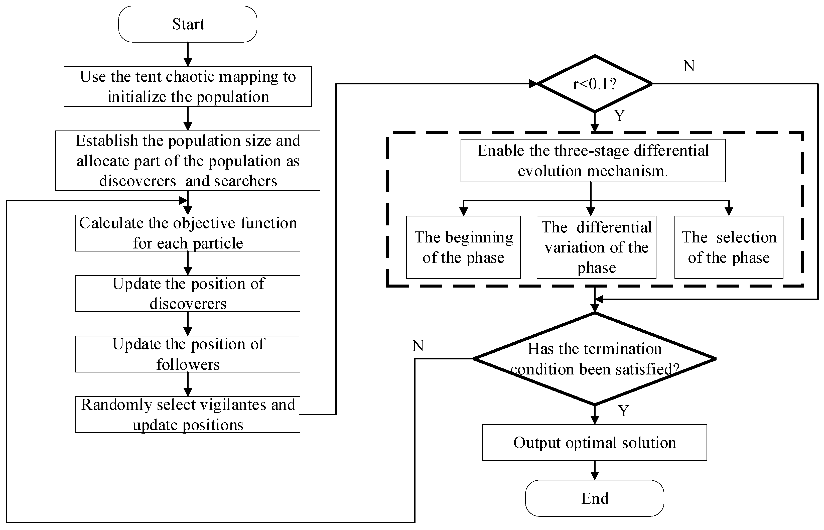
The flowchart depicting the process of the ISSA-PSO algorithm is illustrated in Figure 2.

3.5. Function Test and Result Analysis

(1) Parameter setting

This section uses the Matlab 2019b platform to verify and analyze the computational performance of the ISSA-PSO algorithm to test functions. All the comparison algorithms are set to a population of 30, with 200 iteration times.

(2) Test function

In order to verify the performance of the algorithm, this paper selects four standard test functions for calculation, which are shown in

Table 1. Test function.

Functions	Dimension	Range	Optimum
$f_1\left(x\right)={\displaystyle {\displaystyle \sum }_{i=1}^{30}}i{x}_i^4+ \mathrm{random} [0, 1)\hspace{1em}-1.28\le x_i\le 1.28$	30	[−100, 100]	0
$f_2\left(x\right)={{\displaystyle \sum }}_{i=1}^{30}\left|x_i\right|+{{\displaystyle \prod }}_{i=1}^{30}\left|x_i\right|$	30	[−10, 10]	0
$f_3\left(x\right)=-20exp\left(-0.2\sqrt{\frac{1}{30}{\displaystyle {\displaystyle \sum }_{i=1}^{30}}{x}_i^2}\right)-exp\left(\frac{1}{30}{\displaystyle {\displaystyle \sum }_{i=1}^{30{\sum }_i}}cos 2\pi x_i\right)+20+e$	30	[−32, 32]	8.88 × 10−15
$f_4\left(x\right)=\frac{1}{4000}{\displaystyle {\displaystyle \sum }_{i=1}^{30}}{x}_i^2-{\displaystyle {\displaystyle \prod }_{i=1}^{30\prod \left(\frac{x_i}{\sqrt{i}}\right)}}cos\left(\frac{x_i}{\sqrt{i}}\right)+1$	30	[−50, 50]	0

. To further validate the speed information of the algorithm, the iterative speed of the proposed ISSA-PSO algorithm is compared with that of the SSA, SSA-PSO, GWO, WOA, and SCA on four test functions, as shown in Figure 3, Figure 4, Figure 5 and Figure 6. From the illustration, it can be observed that ISSA-PSO exhibits remarkable performance advantages for unimodal test functions. Therefore, the ISSA-PSO algorithm consistently exhibits the fastest iteration speed when convergence reaches the optimal value.

4. Simulation Results

In order to assess the effectiveness of the improved algorithm in terms of optimization performance, the paper utilizes the IEEE 33-node system and the practical 22-node system for verification. Firstly, the pre-optimized data of each node are obtained by utilizing power flow calculation in the node system. Subsequently, optimization is carried out using the SSA, SSA-PSO, and ISSA-PSO algorithms, respectively. The suitable reactive power compensation devices are selected for the node system applying the above three algorithms. Finally, to further validate the feasibility of the proposed method, the network losses and node voltage are ultimately compared using the SSA, SSA-PSO, and ISSA-PSO algorithms.

4.1. IEEE 33-Node System Simulation Results

The IEEE 33-node system, as depicted in Figure 7, consists of 32 branches and 33 nodes. The five contact switch branches are, respectively, labeled as follows: 8–21, 9–15, 12–22, 18–33, and 25–29. Node 1 is the equilibrium node, while the remaining 32 nodes are load nodes. The three-phase reference power value is 10 MVA, the reference voltage is 12.66 kV, and the total load in the nodal system is 3415 + j2300 kVA.

This paper aims to compensate for reactive power at appropriate nodes in the system, taking into account the loads and voltages on each line as depicted in the diagram. The impedance data for the branches are assumed to be nominal. This paper employs the Newton–Raphson method to perform power flow calculations on a nodal system. Once the power flow calculation is completed, the voltage values corresponding to each node can be obtained prior to optimization, as shown in

Table 2. Voltage of each node in the IEEE 33-node system before optimization.

Node Number	Node Voltage	Node Number	Node Voltage
1	1	18	0.9131
2	0.9970	19	0.9965
3	0.9829	20	0.9929
4	0.9755	21	0.9922
5	0.9681	22	0.9916
6	0.9497	23	0.9794
7	0.9462	24	0.9727
8	0.9413	25	0.9694
9	0.9351	26	0.9477
10	0.9292	27	0.9452
11	0.9284	28	0.9337
12	0.9269	29	0.9255
13	0.9208	30	0.9220
14	0.9185	31	0.9178
15	0.9171	32	0.9169
16	0.9157	33	0.9166
17	0.9137	-	-

.

From Table 2, it is evident that the minimum amplitude manifests at node 18, with a voltage of 0.9131 p.u., while the maximum amplitude manifests at node 2, with a voltage of 0.9970 p.u. The voltage value at the last node in the system is 0.9166 p.u., and the average voltage for the entire system is 0.949 p.u. By analyzing load flow calculations on the standard IEEE 33-node system, there are certain issues pertaining to the overall voltage levels throughout the entire network. The voltage levels fall short of the desired ideals, thereby requiring appropriate compensation measures to enhance the active power within the power system.

The paper adopts the SSA, SSA-PSO algorithm, and ISSA-PSO algorithm to optimize the MORPO model, selecting an initial population size of 30 (the population size of producers accounts for 30 percent of the total population size) and a maximum iteration count of 100; the learning factor is c1 = 2 and c2 = 2, and the inertia weight is $\omega$ = 0.9. The results are shown in Figure 8, Figure 9 and Figure 10.

Figure 8, Figure 9 and Figure 10 illustrate the three-dimensional data optimized by the algorithm proposed in this manuscript for three different objective functions, wherein the x-axis in the graph represents the total active power loss of the optimized nodes, while the y-axis represents the total capacity of the optimized capacitor banks at each node. The z-axis represents the total voltage deviation of the optimized nodes. However, despite the ability of three-dimensional images to fully showcase optimized data, the contrast effect is not particularly prominent. The following sections will individually apply the SSA, the SSA-PSO algorithm, and the ISSA-PSO algorithm to objective functions in detail to validate the effectiveness of the proposed method in this article.

To determine the appropriate compensation nodes and capacities, a parallel capacitor bank is used to switch and compensate for the power at six nodes. The step size for compensation power is 50 kvar. These six nodes are designated as $Q_1$, $Q_2$, $Q_3$, …, $Q_6$.

Table 3. The quantity of compensating capacitors for different optimization algorithms.

Compensation Device Number	SSA		SSA-PSO		ISSA-PSO
	Investment Nodes	Input Quantity	Investment Nodes	Input Quantity	Investment Nodes	Input Quantity
$Q_1$	10	3	3	0	3	0
$Q_2$	16	4	9	3	7	2
$Q_3$	24	0	15	4	14	6
$Q_4$	31	7	30	8	31	8
$Q_5$	32	5	32	3	32	0
$Q_6$	33	0	33	1	33	2

provides the results of the placement and quantity of compensating capacitors based on the SSA, SSA-PSO, and ISSA-PSO algorithms.

Among the selected six nodes, the effect of reactive power compensation on the IEEE 33-node system is found to be the most optimal using ISSA-PSO algorithms. And it can be seen that the ISSA-PAO-calculated compensation capacity is the lowest, which can significantly reduce the system cost in practical applications. In the process of RPO, the magnitude of network loss is a crucial indicator to measure the success of reactive power optimization. To confirm the effectiveness of the method proposed in this paper, the optimization of the objective function using the SSA, SSA-PSO, and ISSA-PSO algorithms is compared. The comparison graph of network loss optimization for the IEEE 33-node system is depicted in Figure 11.

Table 4. Total network loss optimization results.

Optimization Method	Before Optimization	SSA	SSA-PSO	ISSA-PSO
Total network loss (kW)	202.7	159.4	139.0	136.4
Network loss reduction rate (%)	-	21.36	31.43	32.71

presents the optimized results of the total network loss.

From Figure 11, it can be seen that although all three optimization techniques demonstrate favorable effects on network loss reduction, the proposed ISSA-PSO algorithm exhibits the most remarkable reduction. Notably, cables 2, 5, and 27 present significant decreases in network loss, thereby showcasing the excellent optimization efficacy of the ISSA-PSO algorithm. Furthermore, it is evident from Table 4 that the ISSA-PSO method achieves lower network losses compared to the other two methods. Moreover, as indicated by the findings in reference [30], an enhanced PSO algorithm is able to reduce network losses by approximately 11%. In contrast, the implementation of the proposed optimization method in this paper results in a decrease of approximately 33% in network losses, showcasing a significantly superior optimization effect compared with reference [30]. Therefore, the proposed approach demonstrates an excellent reactive power optimization capability.

In the process of RPO, another objective function to gauge the effectiveness of the optimization is the magnitude of node voltages. The comparative diagram of voltage for each node in the optimized system is illustrated in Figure 12.

As depicted in Figure 12, the minimum bus voltage in the absence of RPO stands at 0.9131 p.u. (located at node 18); nevertheless, it elevates to 0.9644 p.u. after employing the methods elucidated in this passage for optimization. Aside from node 18, it is apparent from the graph that other nodes in the system have shown favorable optimization effects. To facilitate a more intuitive and comprehensive comparison between the voltages before and after optimization, the average voltage of all nodes in the overall node line is calculated. The calculated results indicate that the average node voltages after optimization are 0.9658, 0.9655, and 0.9748 utilizing the SSA, SSA-PSO, and ISSA-PSO algorithms, respectively. Moreover, the proposed approach in this paper yields the best optimization effect, with an average node voltage increase of 2.7% after optimization. Hence, the utilization of the ISSA-PSO algorithm for RPO in the standard IEEE 33-node distribution network has yielded better outcomes compared with the other two methods.

4.2. The Practical 22 Node System Simulation Results

In order to further validate the effectiveness of the proposed method in a comprehensive system, the practical 22-node system has been selected for evaluation. The practical 22-node system represented a small portion of an agricultural distribution network within the Eastern Power Distribution system in India, wherein the base voltage stands at 11 kV [38]. The total reactive power load in the system is 657.4 kvar, and active power loss without compensation is 17.69 kW. Among these nodes, node 1 serves as the equilibrium point, while the remaining 21 nodes represent the load nodes. The three-phase reference power value is set at 10 MVA, and the reference voltage at the primary end of the power network is 12.66 kV. Furthermore, the total load within the node system amounts to 662.31 + j657.40 kVA. The practical 22-node system is depicted in Figure 13.

Similar to the IEEE 33-node system, the system is compensated with reactive power compensation devices at the appropriate nodes, taking into account the loads and voltage conditions along each line depicted in the diagram. The average voltage is taken as per unit value. The voltage values corresponding to each individual node are shown in

Table 5. Voltage of each node in the practical 22-node system before optimization.

Node Number	Node Voltage	Node Number	Node Voltage
1	1	12	0.9831
2	0.9969	13	0.9808
3	0.9969	14	0.9756
4	0.9926	15	0.9756
5	0.9925	16	0.9753
6	0.9919	17	0.9743
7	0.9919	18	0.9743
8	0.9918	19	0.9733
9	0.9875	20	0.9731
10	0.9875	21	0.9730
11	0.9831	22	0.9729

before optimization.

Analyzing the results presented in Table 5, it becomes evident that the voltage levels within the practical 22-node system are suboptimal in nature. The overall active power loss within the system amounts to 17.7 kW, with the lowest magnitude occurring at node 22, where the voltage value stands at 0.9729 p.u. The collective mean voltage of the system amounts to 0.9838 p.u.

The paper adopts the SSA, SSA-PSO algorithm, and ISSA-PSO algorithm to optimize the MORPO model. The results are shown in Figure 14, Figure 15 and Figure 16.

In Figure 14, Figure 15 and Figure 16, the system is analogous to the practical 22-node system: the x, y, and z axes represent the total active power loss of the optimized nodes, the total capacity of the optimized capacitor banks at each node, and the total voltage deviation of the optimized nodes. Due to the inability to showcase specific optimization effects in Figure 14, Figure 15 and Figure 16, the following sections will compare the results obtained after optimizing the objective function using the SSA, the SSA-PSO algorithm, and the ISSA-PSO algorithm.

Similar to the IEEE 33-node system, the step size for compensation power is 50 kvar. These six nodes are designated as $Q_1$, $Q_2$, $Q_3$, …, $Q_6$.

Table 6. The quantity of compensating capacitors for different optimization algorithms.

Compensation Device Number	SSA		SSA-PSO		ISSA-PSO
	Investment Nodes	Input Quantity	Investment Nodes	Input Quantity	Investment Nodes	Input Quantity
$Q_1$	2	0	2	0	2	0
$Q_2$	2	0	2	0	3	0
$Q_3$	2	1	2	0	5	1
$Q_4$	6	1	3	0	8	1
$Q_5$	16	1	8	0	17	2
$Q_6$	20	4	19	4	21	2

showcases the placement and quantity of compensating capacitors in various scenarios.

Among the selected six nodes, the effect of reactive power compensation for the practical 22-node system is found to be the most optimal by applying the ISSA-PSO algorithm. Moreover, the results of the compensation capacity using the ISSA-PSO algorithm are still the lowest in the case of the practical 22-node system, resulting in a significant reduction in system cost in practical applications. The comparison graph of network loss optimization for the practical 22-node system is depicted in Figure 17.

Table 7. Total network loss optimization results.

Optimization Method	Before Optimization	SSA	SSA-PSO	ISSA-PSO
Total network loss (kW)	17.7	10.2	10.0	9.9
Network loss reduction rate (%)	-	42.37	43.50	44.07

shows the optimization results of total network loss.

As can be seen from Figure 17, although all three optimization techniques show favorable effects on network loss reduction, the proposed ISSA-PSO algorithm shows the most significant reduction. It is worth noting that cables 3, 5, 10, and 12 show a significant reduction in network loss, thus demonstrating the excellent optimization efficiency of the ISSA-PSO algorithm. Furthermore, Table 7 shows the optimization results of total network loss after applying the SSA, SSA-PSO, and ISSA-PSO algorithms in an actual 22-bus system. From Table 7, it is evident that the network loss is 17.7 kW before optimization. After applying the SSA, SSA-PSO, and ISSA-PSO algorithms, a noticeable decrease in power loss can be observed. Importantly, the ISSA-PSO algorithm demonstrates the most significant reduction, with an impressive decline of 44.07%. The effectiveness of this approach surpasses that of other algorithms, demonstrating better optimization results. The comparative diagram of voltage for each node in the optimized system is illustrated in Figure 18.

As depicted in Figure 18, the minimum bus voltage in the absence of RPO stands at 0.9729 p.u. (located at node 22). Nevertheless, it elevates to 0.9879 p.u., corresponding to the implementation of the proposed resolution. Aside from node 22, it is apparent from the graph that other nodes in the system have shown favorable optimization effects. To facilitate a more intuitive and comprehensive comparison between the voltages before and after optimization, the average voltage of all nodes in the overall node line is calculated. The calculated results indicate that the average node voltages after optimization are 0.9882, 0.9882, and 0.9921 when employing SSA, SSA-PSO, and ISSA-PSO, respectively. Furthermore, the proposed approach in this paper yields the best optimization effect, with an average node voltage increase of 0.84% after optimization. Therefore, the ISSA-PSO algorithm has better optimization outcomes in the practical 22-node system.

It should be noted that the simulation verification in this article is carried out within the scope of conventional power distribution grids, assuming only sinusoidal quantities for voltage and current waveforms. However, in the actual power grid, the voltage and current waveforms are often influenced by various power quality disturbances, leading to nonsinusoidal waveforms in the actual power grid. These power quality disturbances include, but are not confined to, higher-order harmonics, subharmonics, and harmonic distortions, among others, that can influence the standard functioning of the electricity network and the efficiency of machinery [39,40,41]. Therefore, the upcoming research will focus on the implications of harmonic distortion and voltage distortion issues on the power grid.

5. Conclusions

This paper establishes the MORPO model in the distribution network including reactive power loss, reactive power devices, and the total sum of node voltage deviations. Based on the SSA and PSO algorithm, the ISSA-PSO algorithm is proposed for converging to a global optimal solution effectively. Compared with the SSA and SSA-PSO, the proposed model has exhibited promising results in the IEEE 33-node system and the practical 22-node system. The simulation results show that the total network losses of the IEEE 33-node system decreased from 202.7 kW to 136.4 kW, representing a reduction of 32.71%. In terms of node voltage, the average voltage magnitude of the lines increases from 0.9485 p.u. to 0.9748 p.u. Similarly, the total network losses of the practical 22-node system decreased from 17.7 kW to 9.9 kW, resulting in a reduction of 44.07%. Regarding node voltage, the average voltage magnitude of the lines increases from 0.9838 p.u. to 0.9921 p.u. Therefore, the proposed algorithm can effectively improve optimization performance by reducing active power loss and enhancing voltage levels simultaneously. However, the simulation verification in this study is conducted within conventional power systems without taking into account the voltage nonliterary issues that arise from the integration of distributed energy resources into the grid. Our future research will primarily focus on investigating the effects of harmonic distortion and voltage imbalance in distribution networks on reactive power optimization.

References

1. Hu, W.; Guo, Q.; Wang, W.; Wang, W.; Song, S. Loss Reduction Strategy and Evaluation System Based on Reasonable Line Loss Interval of Transformer Area. Appl. Energy 2022, 306, 118123. [Google Scholar] [CrossRef]
2. Capitanescu, F.; Wehenkel, L. Experiments with the Interior-Point Method for Solving Large Scale Optimal Power Flow Problems. Electr. Power Syst. Res. 2013, 95, 276–283. [Google Scholar] [CrossRef]
3. Liu, X.; Zhang, P.; Fang, H.; Zhou, Y. Multi-Objective Reactive Power Optimization Based on Improved Particle Swarm Optimization with ε-Greedy Strategy and Pareto Archive Algorithm. IEEE Access 2021, 9, 65650–65659. [Google Scholar] [CrossRef]
4. Xie, Z.; Chen, Y.; Wu, W.; Gong, W.; Guerrero, J.M. Stability Enhancing Voltage Feed-Forward Inverter Control Method to Reduce the Effects of Phase-Locked Loop and Grid Impedance. IEEE J. Emerg. Sel. Top. Power Electron. 2021, 9, 3000–3009. [Google Scholar] [CrossRef]
5. Chen, G.; Qian, J.; Zhang, Z.; Li, S. Application of Modified Pigeon-Inspired Optimization Algorithm and Constraint-Objective Sorting Rule on Multi-Objective Optimal Power Flow Problem. Appl. Soft Comput. 2020, 92, 106321. [Google Scholar] [CrossRef]
6. Ayan, K.; Kılıç, U. Artificial Bee Colony Algorithm Solution for Optimal Reactive Power Flow. Appl. Soft Comput. 2012, 12, 1477–1482. [Google Scholar] [CrossRef]
7. Wenxue, L.; Luhua, X.; Changhui, M.; Wenbo, L. Multi-Objective Reactive Power Optimization of Hybrid AC/DC Power System Considering Power System Uncertainty. J. Phys. Conf. Ser. 2019, 1187, 022039. [Google Scholar] [CrossRef]
8. Eghbal, M.; Yorino, N.; Zoka, Y.; El-Araby, E.E. Application of Multi-Objective Evolutionary Optimization Algorithms to Reactive Power Planning Problem. IEEJ Trans. Electr. Electron. Eng. 2009, 4, 625–632. [Google Scholar] [CrossRef]
9. Basu, M. Multi-Objective Optimal Reactive Power Dispatch Using Multi-Objective Differential Evolution. Int. J. Electr. Power Energy Syst. 2016, 82, 213–224. [Google Scholar] [CrossRef]
10. Inoue, M.; Sadamoto, T.; Arahata, M.; Chakrabortty, A. Optimal Power Flow Design for Enhancing Dynamic Performance: Potentials of Reactive Power. IEEE Trans. Smart Grid 2021, 12, 599–611. [Google Scholar] [CrossRef]
11. Chuong, T.D. Exact Relaxations for Parametric Robust Linear Optimization Problems. Oper. Res. Lett. 2019, 47, 105–109. [Google Scholar] [CrossRef]
12. Zhang, C.; Liu, Q.; Huang, S.; Zhou, B.; Cheng, L.; Gao, L.; Li, J. Reactive Power Optimization under Interval Uncertainty of Renewable Power Generation Based on a Security Limits Method. Int. J. Electr. Power Energy Syst. 2021, 130, 106894. [Google Scholar] [CrossRef]
13. Mangoli, M.K.; Lee, K.Y.; Moon Park, Y. Optimal Real and Reactive Power Control Using Linear Programming. Electr. Power Syst. Res. 1993, 26, 1–10. [Google Scholar] [CrossRef]
14. Chen, J.; Huang, L.; Lv, Y.; Wen, C.-F. Optimality Conditions of Robust Convex Multiobjective Optimization via ε -Constraint Scalarization and Image Space Analysis. Optimization 2020, 69, 1849–1879. [Google Scholar] [CrossRef]
15. Duman, S.; Güvenç, U.; Sönmez, Y.; Yörükeren, N. Optimal Power Flow Using Gravitational Search Algorithm. Energy Convers. Manag. 2012, 59, 86–95. [Google Scholar] [CrossRef]
16. Zhao, B.; Guo, C.X.; Cao, Y.J. A Multiagent-Based Particle Swarm Optimization Approach for Optimal Reactive Power Dispatch. IEEE Trans. Power Syst. 2005, 20, 1070–1078. [Google Scholar] [CrossRef]
17. Shaheen, M.A.M.; Hasanien, H.M.; Alkuhayli, A. A Novel Hybrid GWO-PSO Optimization Technique for Optimal Reactive Power Dispatch Problem Solution. Ain Shams Eng. J. 2021, 12, 621–630. [Google Scholar] [CrossRef]
18. Attia, A.-F.; El Sehiemy, R.A.; Hasanien, H.M. Optimal Power Flow Solution in Power Systems Using a Novel Sine-Cosine Algorithm. Int. J. Electr. Power Energy Syst. 2018, 99, 331–343. [Google Scholar] [CrossRef]
19. Sun, L.; Si, S.; Ding, W.; Wang, X.; Xu, J. Multiobjective Sparrow Search Feature Selection with Sparrow Ranking and Preference Information and Its Applications for High-Dimensional Data. Appl. Soft Comput. 2023, 147, 110837. [Google Scholar] [CrossRef]
20. Mehdinejad, M.; Mohammadi-Ivatloo, B.; Dadashzadeh-Bonab, R.; Zare, K. Solution of Optimal Reactive Power Dispatch of Power Systems Using Hybrid Particle Swarm Optimization and Imperialist Competitive Algorithms. Int. J. Electr. Power Energy Syst. 2016, 83, 104–116. [Google Scholar] [CrossRef]
21. Zhang, C.-X.; Zhou, K.-Q.; Ye, S.-Q.; Zain, A.M. An Improved Cuckoo Search Algorithm Utilizing Nonlinear Inertia Weight and Differential Evolution for Function Optimization Problem. IEEE Access 2021, 9, 161352–161373. [Google Scholar] [CrossRef]
22. Raha, S.B.; Mandal, K.K.; Chakraborty, N. Hybrid SMES Based Reactive Power Dispatch by Cuckoo Search Algorithm. IEEE Trans. Ind. Appl. 2019, 55, 907–917. [Google Scholar] [CrossRef]
23. Liu, Y.; Ćetenović, D.; Li, H.; Gryazina, E.; Terzija, V. An Optimized Multi-Objective Reactive Power Dispatch Strategy Based on Improved Genetic Algorithm for Wind Power Integrated Systems. Int. J. Electr. Power Energy Syst. 2022, 136, 107764. [Google Scholar] [CrossRef]
24. Qian, J.; Wang, P.; Pu, C.; Chen, G. Joint Application of Multi-Object Beetle Antennae Search Algorithm and BAS-BP Fuel Cost Forecast Network on Optimal Active Power Dispatch Problems. Knowl.-Based Syst. 2021, 226, 107149. [Google Scholar] [CrossRef]
25. Deb, K.; Pratap, A.; Agarwal, S.; Meyarivan, T. A Fast and Elitist Multiobjective Genetic Algorithm: NSGA-II. IEEE Trans. Evol. Computat. 2002, 6, 182–197. [Google Scholar] [CrossRef]
26. Jamal, R.; Men, B.; Khan, N.H. A Novel Nature Inspired Meta-Heuristic Optimization Approach of GWO Optimizer for Optimal Reactive Power Dispatch Problems. IEEE Access 2020, 8, 202596–202610. [Google Scholar] [CrossRef]
27. Zhang, J.; Wang, X.; Ma, L. An Optimal Power Allocation Scheme of Microgrid Using Grey Wolf Optimizer. IEEE Access 2019, 7, 137608–137619. [Google Scholar] [CrossRef]
28. Sathish Kumar, K.; Jayabarathi, T. Power System Reconfiguration and Loss Minimization for an Distribution Systems Using Bacterial Foraging Optimization Algorithm. Int. J. Electr. Power Energy Syst. 2012, 36, 13–17. [Google Scholar] [CrossRef]
29. Kennedy, J.; Eberhart, R. Particle Swarm Optimization. In Proceedings of the ICNN’95—International Conference on Neural Networks, Perth, Australia, 27 November–1 December 1995; Volume 4, pp. 1942–1948. [Google Scholar]
30. Mourtzis, D.; Angelopoulos, J. Reactive Power Optimization Based on the Application of an Improved Particle Swarm Optimization Algorithm. Machines 2023, 11, 724. [Google Scholar] [CrossRef]
31. Chen, G.; Liu, L.; Song, P.; Du, Y. Chaotic Improved PSO-Based Multi-Objective Optimization for Minimization of Power Losses and L Index in Power Systems. Energy Convers. Manag. 2014, 86, 548–560. [Google Scholar] [CrossRef]
32. Cai, Y.; Liu, J.; Gao, N. Research on Reactive Power Optimization Control Method for Distribution Network with DGs Based on Improved Second-Order Oscillating PSO Algorithm. J. Control Sci. Eng. 2023, 2023, 5813277. [Google Scholar] [CrossRef]
33. Wang, Y.; Dai, S.; Liu, P.; Zhao, X. A Hybrid Particle Swarm Optimization with Butterfly Optimization Algorithm Based Maximum Power Point Tracking for Photovoltaic Array under Partial Shading Conditions. Sustainability 2023, 15, 12402. [Google Scholar] [CrossRef]
34. Xue, J.; Shen, B. A Novel Swarm Intelligence Optimization Approach: Sparrow Search Algorithm. Syst. Sci. Control Eng. 2020, 8, 22–34. [Google Scholar] [CrossRef]
35. Dong, J.; Dou, Z.; Si, S.; Wang, Z.; Liu, L. Optimization of Capacity Configuration of Wind–Solar–Diesel–Storage Using Improved Sparrow Search Algorithm. J. Electr. Eng. Technol. 2022, 17, 1–14. [Google Scholar] [CrossRef]
36. Tang, A.; Zhou, H.; Han, T.; Xie, L. A Chaos Sparrow Search Algorithm with Logarithmic Spiral and Adaptive Step for Engineering Problems. Comput. Model. Eng. Sci. 2022, 130, 331–364. [Google Scholar] [CrossRef]
37. Ren, L.; Zhang, W.; Ye, Y.; Li, X. Hybrid Strategy to Improve the High-Dimensional Multi-Target Sparrow Search Algorithm and Its Application. Appl. Sci. 2023, 13, 3589. [Google Scholar] [CrossRef]
38. Ramalinga Raju, M.; Ramachandra Murthy, K.V.S.; Ravindra, K. Direct Search Algorithm for Capacitive Compensation in Radial Distribution Systems. Int. J. Electr. Power Energy Syst. 2012, 42, 24–30. [Google Scholar] [CrossRef]
39. Kuwalek, P.; Wiczynski, G. Dependence of Voltage Fluctuation Severity on Clipped Sinewave Distortion of Voltage. IEEE Trans. Instrum. Meas. 2021, 70, 2006008. [Google Scholar] [CrossRef]
40. Kuwałek, P.; Wiczyński, G. Problem of Total Harmonic Distortion Measurement Performed by Smart Energy Meters. Meas. Sci. Rev. 2022, 22, 1–10. [Google Scholar] [CrossRef]
41. Dyer, S.; Dyer, J. Distortion: Total Harmonic Distortion in an Asymmetrically Clipped Sinewave. IEEE Instrum. Meas. Mag. 2011, 14, 48–51. [Google Scholar] [CrossRef]
Figure 1. SSA-PSO algorithm flowchart.
Energies 17 02001 g001
Figure 2. ISSA-PSO algorithm flowchart.
Energies 17 02001 g002
Figure 3. Test function f 1 x .
Energies 17 02001 g003
Figure 4. Test function f 2 x .
Energies 17 02001 g004
Figure 5. Test function f 3 x .
Energies 17 02001 g005
Figure 6. Test function f 4 x .
Energies 17 02001 g006
Figure 7. IEEE 33-node system chart.
Energies 17 02001 g007
Figure 8. Optimized results based on SSA.
Energies 17 02001 g008
Figure 9. Optimized results based on SSA-PSO algorithm.
Energies 17 02001 g009
Figure 10. Optimized results based on ISSA-PSO algorithm.
Energies 17 02001 g010
Figure 11. Comparison chart of network loss optimization in IEEE 33-node system.
Energies 17 02001 g011
Figure 12. Comparison chart of node voltages in IEEE 33-node system.
Energies 17 02001 g012
Figure 13. The diagram of the practical 22-node system.
Energies 17 02001 g013
Figure 14. Optimized results based on SSA.
Energies 17 02001 g014
Figure 15. Optimized results based on SSA-PSO algorithm.
Energies 17 02001 g015
Figure 16. Optimized results based on ISSA-PSO algorithm.
Energies 17 02001 g016
Figure 17. Comparison chart of system loss optimization in the practical 22-node system.
Energies 17 02001 g017
Figure 18. Comparison chart of node voltages in the practical 22-node system.
Energies 17 02001 g018