Study on Traveling Wave Fault Localization of Transmission Line Based on NGO-VMD Algorithm

Abstract

To address the challenge of inaccurate fault location of variational mode decomposition (VMD) in practical engineering, due to poor choice of mode decomposition number K and quadratic penalty factor α, a traveling wave fault location method using Northern Goshawk optimization algorithm (NGO) to optimize VMD was proposed. First, the NGO algorithm is used to optimize VMD, and the optimal K and α are obtained. Secondly, the optimal parameters are inputted into VMD for fault signal decomposition, and the eigenmode components are obtained. Due to the difficulty of identification of the traveling wave head in the process of traveling wave propagation, Hilbert transform is used to determine the time of initial arrival of the traveling wave head at both ends of the line, and the fault location is precisely calculated by using the two-ended traveling wave fault detection formula. Finally, simulation experiments are carried out to verify the accuracy of the proposed location method, which shows that the proposed location method can locate the fault more accurately and has good engineering application value.

1. Introduction

As key building blocks of the power transmission system, transmission lines carry out the critical task of power transmission. They are also susceptible to geomorphologic and weather conditions; once the failure occurs, this poses a significant threat to the security and stability of the power grid. It is imperative to pinpoint faults swiftly and precisely, in order to take timely measures to repair and restore the power supply [1,2]. Therefore, investigating fault localization using traveling waves in transmission lines is crucial for enhancing the dependability and robustness of the power system.

A significant number of researchers have dedicated their efforts to advancing transmission line fault localization technologies. Concomitant with the swift progress in microelectronics, this area of study has garnered increasing interest from the scientific community. Nowadays, there are three main categories of commonly used fault localization methods: the impedance method, traveling wave method, and artificial intelligence method.

The principle of the impedance method is that when a fault occurs in a power system, the circuit impedance change near the fault point can be calculated by measuring the voltage and current, and the fault point impedance is directly proportional to the distance, so the fault location can be deduced based on the impedance value [3]. The principle of the impedance method is relatively simple and, compared with some advanced fault location techniques, impedance ranging does not require expensive specialized equipment and complex software, so the cost is low. However, impedance ranging is usually unable to detect and locate transient faults, and the accuracy of impedance ranging is affected by power system parameters (e.g., line length, load conditions, transformer errors, etc.) [4,5].

The traveling wave method is widely used in transmission line fault location, by sending electromagnetic pulse signals into the measured conductor or cable and using the reflection characteristics of the signal to determine the length of the conductor or cable and the potential fault location [6,7]. Depending on the number of measurement points employed, traveling wave fault location techniques can be categorized into single-ended and double-ended traveling wave methods. When only the electrical quantity data at one end of the fault point is utilized for measurement, it is called a single-end measurement method; relatively, if the electrical quantity data at both ends are used, it is called a double-end measurement method. Literature [8] proposed an innovative spatio-temporal full-dimensional single-ended traveling wave ranging technique, which effectively reduces the error of the traditional single-ended traveling wave localization technique. One study [9] improved the double-ended traveling wave ranging method by deploying high-frequency sensors for accurate wave head sampling and introducing the concept of correction wave. Another study [10] deployed multiple traveling wave detection devices at key locations of overhead lines and ground cable lines to solve the ranging errors caused by transient traveling wave signal attenuation.

The artificial intelligence method of fault location builds a feature volume database by collecting actual fault data, studies the correlation between fault transient fluctuation and distance, and trains the data using artificial intelligence techniques to build a fault location model. Once a fault occurs, the fault location can be calculated by simply inputting the detected fault information into this model. One study [11] proposed an improved algorithm for AFSA-PSO by combining particle swarm optimization (PSO) techniques with the Artificial Fish Swarm algorithm (AFSA) and applied the algorithm to the fault location model of distribution network. Another study [12] proposed a whale optimization algorithm enhanced by multiple strategies, and another [13] merged the simulated annealing algorithm with a refined Newtonian optimization approach.

In contrast to the impedance method, the traveling wave ranging technique offers higher accuracy and is less affected by the characteristics of the transmission line. At the same time, the artificial intelligence method can optimize the traditional algorithms and has strong computational ability, so this study employs a combination of artificial intelligence techniques and the double-ended traveling wave ranging method to analyze fault-induced traveling wave signals, thereby enhancing the precision of fault localization.

In the realm of fault localization utilizing the double-ended traveling wave method, two principal challenges emerge:

(1)

Detection of faulty traveling wave signals

The precise identification of the mutation point within the fault traveling wave signal is crucial for enhancing the accuracy of fault localization in transmission lines. When a fault occurs in a transmission line, the traveling wave undergoes refraction and reflection at the fault point during propagation. Moreover, the collected fault current signals may be corrupted by noise, making the detection of the fault traveling wave signals challenging [14].

(2)

Inconsistent traveling wave velocity

The velocity of the traveling wave plays a pivotal role in the fault location for transmission lines, the choice of wave velocity is directly related to the accuracy of location. In actual power systems, the structure and parameters of transmission lines are not uniform, leading to variations in wave velocity within the lines. Additionally, environmental factors can also cause changes in wave velocity.

In response to the difficult problem of faulty traveling wave signal detection, this paper introduces an innovative method for detecting fault signals. This method begins by employing the Northern Goshawk optimization algorithm (NGO) to refine the optimization of the two critical parameters in the variational mode decomposition (VMD) method, namely, the number of modal decomposition layers, K, and the penalty factor, α, then the optimized VMD decomposes the line mode component of the fault current traveling wave after phase mode transformation into a number of intrinsic modal function (IMF) components; finally, performing the Hilbert transform on the IMF1 component generates its instantaneous spectrogram. The initial frequency variation point on this spectrogram coincides with the moment of the traveling wave’s initial arrival. To address the difficult problem of inconsistent travelling wave speed, this paper introduces an enhanced double-ended traveling wave ranging method that leverages relative time differences to obviate the challenges associated with wave speed variability and clock synchronization. The method requires only the knowledge of the transmission line’s horizontal distance, the initial fault occurrence time, and the arrival time data of the traveling wave at both ends of the line, for ranging purposes. Section 2 of this paper introduces the fundamental principles of the fault location algorithm. Section 3 introduces the fault location scheme based on the NGO-VMD-HHT algorithm. Section 4 simulates the proposed ranging scheme and analyzes its performance under various fault conditions.

2. Basic Theory

2.1. Fundamentals of the Hilbert–Huang Transformation

The Hilbert–Huang Transform (HHT) is an adaptive time-frequency analysis method designed specifically for non-linear and non-smooth signals. It consists of two main components: empirical mode decomposition (EMD) and Hilbert transform (HT). Empirical mode decomposition is responsible for decomposing the signal into a set of intrinsic mode functions (IMFs) [15,16]. After IMF generation, the HHT analyzes each IMF using the Hilbert transform.

For any continuous time signal $x\left(t\right)$, its Hilbert transform $Y\left(t\right)$ can be obtained:

$$Y(t)=\frac{1}{\pi }{\displaystyle \underset{-\infty }{\overset{+\infty }{\int }}\frac{X(t)}{t-\tau }}d\tau$$

(1)

The inverse transformation of Equation (1) is:

$$X(t)=\frac{1}{\pi }{\displaystyle \underset{-\infty }{\overset{+\infty }{\int }}\frac{Y(t)}{t-\tau }}d\tau$$

(2)

The analytical signal is obtained from Equation (2) as:

$$Z(t)=X(t)+jY(t)=A(t)e^{j\theta (t)}$$

(3)

In Equation (3), $A(t)$ represents the instantaneous frequency of the signal and $\theta \left(t\right)$ represents the frequency phase of the signal.

This one:

$$A(t)=\sqrt{X^2(t)+Y^2(t)}$$

(4)

$$\theta (t)=\arctan (\frac{Y(t)}{X(t)})$$

(5)

Another instantaneous parameter $\theta \left(t\right)$ can be derived through:

$$f(t)=\frac{1}{2\pi }\frac{d\theta (t)}{dt}$$

(6)

From Equation (5), it can be obtained that the three instantaneous time parameters, instantaneous amplitude, instantaneous phase and instantaneous frequency of the time signal can be solved by Hilbert–Huang transform.

In general, since high frequency signals contain multiple frequencies, it is difficult to decompose all the frequencies of the signal using only the HHT, so it is necessary to divide the data into IMF first, and to define the instantaneous frequency, the signal function needs to satisfy the following three conditions:

(1)

The function is symmetric throughout the interval of definition of the signaling function;

(2)

The signal function exhibits an identical count of zero-crossings and extremum points;

(3)

The signal function has a local mean of zero.

The IMF needs to have the following conditions:

(1)

In the original signal, the number of zeros is equal to or differs from the number of extreme points by one, i.e., the requirement of Equation (7) is satisfied:

$$\left(Q_z-1\right)\le Q_e\le \left(Q_z+1\right)$$

(7)

(2)

At any given point in time, the signal’s upper and lower envelopes, as determined by its local maximum and minimum points, exhibit a mean value of zero, i.e., Equation (8) is satisfied:

$$\frac{\left[f_{\max }\left(t_i\right)+f_{\min }\left(t_i\right)\right]}{2}=0$$

(8)

In Equation (8), $t_i$ represents any time of the signal, and which is in the domain of definition of the signal time, $f_{\max }\left(t_i\right)$ represents the value of the upper envelope, $f_{\min }\left(t_i\right)$ represents the value of the lower envelope.

2.2. Variational Modal Decomposition

Variational modal decomposition (VMD) is a decomposition method based on signal filtering that decomposes a non-linear, non-smooth signal into a set of vibrational modes of intrinsic frequency and amplitude [17,18]. The VMD algorithm determines the finite bandwidth and optimal center frequency of the intrinsic modal component (IMF) by iterative search, assuming that the signal is divided into K intrinsic modal components, and the bandwidths of the components need to be estimated to satisfy the summation of the minimum, which is constrained by the variational modeling equation:

$$\left\{\begin{array}{l}\underset{{\mu }_k,{\omega }_k}{{\displaystyle \min }}\left\{{\displaystyle \sum _k\left|\right|\mathsf{\partial }(t)\left[\left(\phi (t)+\frac{j}{\pi t}\right)\ast {\mu }_k(t)\right]e^{-j{\omega }_{k}t}}\left|\right|\genfrac{}{}{0ex}{}{2}{2}\right\}\\ s.t.{\displaystyle \sum _k{\mu }_k}=f\end{array}\right.$$

(9)

In Equation (9): $\left\{{\mu }_k\right\}$ is the set of intrinsic modal components; ${\omega }_k$ is the center frequency of each modal component, $f$ is the input signal, $\delta \left(t\right)$ is the impulse function.

Invoking the Lagrange multiplier operator λ can transform the constrained variational problem into an unconstrained variational problem, while the introduction of a quadratic penalty factor α can reduce the interference of Gaussian noise, and the optimal number of intrinsic modal components and the corresponding center frequency can be obtained by searching for the saddle points of the augmented Lagrangian function. The augmented Lagrangian expression is:

$$\begin{array}{l}L\left(\left\{{\mu }_k\right\},\left\{{\omega }_k\right\},\lambda \right)=\alpha {{\displaystyle \sum _k‖{\mathsf{\partial }}_t\left[\left(\delta \left(\mathrm{t}\right)+\frac{\mathrm{j}}{\pi \mathrm{t}}\right){\mu }_{\mathrm{k}}\left(t\right)\right]e^{-j{\omega }_{k}t}‖}}_2^2\\ +{‖f\left(t\right)-{\displaystyle \sum _k{\mu }_k\left(t\right)}‖}_2^2+〈\lambda \left(t\right),f\left(t\right)-{\displaystyle \sum _k{\mu }_k\left(t\right)}〉\end{array}$$

(10)

The expressions for the modal components and center frequency after alternating iterative optimization are:

$${\widehat{\mu }}_k^{n+1}\left(\omega \right)=\left(\widehat{f}\left(\omega \right)-{\displaystyle \sum _{i\ne k}{\widehat{\mu }}_i\left(\omega \right)+\frac{\widehat{\lambda }\left(\omega \right)}{2}}\right)\frac{1}{1+2\alpha {\left(\omega -{\omega }_k\right)}^2}$$

(11)

$${\widehat{\omega }}_k^{n+1}\left(\omega \right)=\frac{{\displaystyle {\int }_0^{\infty }\omega {\left|{\widehat{\mu }}_k\left(\omega \right)\right|}^{2}d\omega }}{{\displaystyle {\int }_0^{\infty }{\left|{\widehat{\mu }}_k\left(\omega \right)\right|}^{2}d\omega }}$$

(12)

$${\widehat{\lambda }}^{n+1}\left(\omega \right)\leftarrow {\widehat{\lambda }}^n\left(\omega \right)+\gamma \left[\widehat{f}\left(\omega \right)-{\displaystyle \sum _k{\widehat{\mu }}_k^{n+1}\left(\omega \right)}\right]$$

(13)

where $\gamma$ is the noise tolerance, ${\widehat{\mu }}_k^{n+1}\left(\omega \right)$, ${\widehat{\omega }}_k^{n+1}\left(\omega \right)$, ${\widehat{\lambda }}^{n+1}\left(\omega \right)$ is the frequency domain expression.

The steps of the VMD algorithm are as follows:

(1)

Initialize the signals to be decomposed $\left\{{\widehat{\mu }}_k^1\right\}$, $\left\{{\widehat{\omega }}_k^1\right\}$, $\left\{{\widehat{\lambda }}^1\right\}$, such that n = 0;

(2)

n = n + 1, execute the loop;

(3)

Updated ${\mu }_k$, ${\omega }_k$ using Equation (11) with Equation (12);

(4)

$k=k+1$, whether the preset value of K is reached. If k is equal to K, the loop is terminated; otherwise, return to step (3) to continue execution;

(5)

According to Equation (13), λ is updated;

(6)

Check if the conditions are met: ${\displaystyle \sum _k{‖{\widehat{\mu }}_k^{n+1}-{\widehat{\mu }}_k^n‖}_2^2/}{‖{\widehat{\mu }}_k^n‖}_2^2<\epsilon$. If it is satisfied, the iteration is terminated and the values of ${\mu }_k$ and ${\omega }_k$ are output; if it is not satisfied, the execution of steps (2) to (5) continues.

2.3. Northern Goshawk Optimization Algorithm

The Northern Goshawk optimization algorithm (NGO) is a natural heuristic algorithm inspired by the hunting behavior of the northern goshawk. The algorithm simulates the way the northern goshawk searches for the best prey during the hunting process, and is able to perform better in various optimization problems [19]. The NGO algorithm is mainly divided into two phases of behavior:

(1)

Prey identification and attack phase

In this phase, the individual randomly selects a target in the search space, uses its position as the target of the attack, and moves the current position towards the target. This stage involves global search to determine the optimal region. Equations (14)–(16) are the mathematical modeling formulas for this phase:

$$P_i=X_k,i=1,2,\cdots ,\mathrm{N},k=1,2,\cdots ,i-1,i+1,\cdots ,\mathrm{N}$$

(14)

$$x_{i,j}^{new,P1}=\left\{\begin{array}{l}{x}_{i,j}+r\left(p_{i,j}-I{x}_{i,j}\right),F_{P_i}\ge F_i\\ x_{i,j}+r\left(x_{i,j}-p_{i,j}\right),F_{P_i}<F_i\end{array}\right.$$

(15)

$$X_i=\left\{\begin{array}{ll}{X}_i^{new,P1},& F_i^{new,P1}<F_i\\ X_i,& F_i^{new,P1}<F_i\end{array}\right.$$

(16)

where $P_i$ denotes the location of the ith northern pallid prey; k is a random integer in the range $\left[1,n\right]$, $X_i^{new,P1}$ is the new state of the ith northern goshawk, $x_{i,j}^{new,{\rm P}1}$ is then its new state in the jth dimension, $F_i^{new,P1}$ is the objective function for that stage. $r$ is a random number of $\left[1,2\right]$, the value of ${\rm I}$ is either 1 or 2, both of which are random numbers in the middle of the search and iteration.

(2)

Prey chase and escape phase

Once the northern goshawk launches an assault on its quarry, the prey will make an effort to escape, prompting the hawk to give chase, the stage is a localized search, to pinpoint the most optimal solution, assuming that the hunting range of the northern goshawk is R, the mathematical model equations of this stage can be expressed by Equations (17)–(19):

$$x_{i,j}^{new,P_2}=x_{i,j}+R\left(2r-1\right)x_{i,j}$$

(17)

$$R=0.02\left(1-\frac{t}{T}\right)$$

(18)

$${{\rm X}}_i=\left\{\begin{array}{l}{{\rm X}}_i^{new,P_2},F_i^{new,P_2}\le F_i\\ X_i,F_i^{new,P_2}\ge F_i\end{array}\right.$$

(19)

where ${{\rm X}}_i^{new,P_2}$ is the new position of the ith northern goshawk in that phase; $x_{i,j}^{new,P_2}$ is the new position of the ith northern goshawk in the jth dimension in that phase, $t$ is the current number of iterations, T is the maximum number of iterations, and $F_i^{new,P_2}$ is the objective function for the stage.

The steps of the NGO algorithm are as follows: initialize the population, complete the iterative process of the algorithm, determine the parameters of the population, the objective function and the optimal solution, repeat the process from (14) to (19) until the completion of the last iteration, and find the optimal solution of the whole process, i.e., the solution of the given optimization.

3. Ranging Scheme Based on NGO-VMD Algorithm

3.1. Phase-Mode Conversion

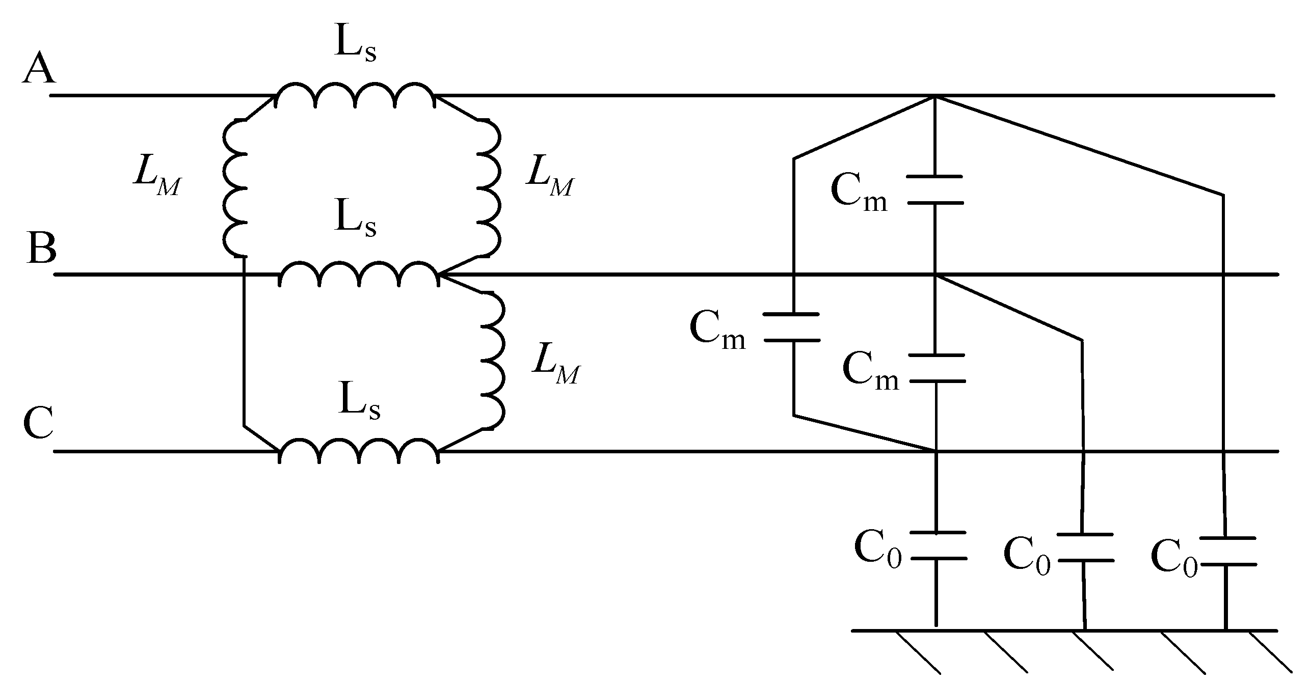
The actual power system transmission lines are three-phase transmission lines between the phase and phase, and phase and ground electromagnetic coupling phenomenon, which will affect the extraction and analysis of the relevant signals [20]. In order to eliminate the phenomenon of electromagnetic coupling, the use of travelling wave ranging method is commonly used, before the use of the phase-mode transform method of decoupling, and then analyzes the independent modulus after decoupling. The equivalent network of electromagnetic coupling for a three-phase system is shown in Figure 1 below.

Currently, the commonly used phase mode transformation matrices are Clarke and Karenbauer transforms, but since these two transformation matrices cannot reflect the characteristics of various fault types through a single modulus, this paper introduces an improved phase-to-mode conversion matrix, designed to address the limitations of conventional phase-mode transformation.

Let the improved phase-mode transformation matrix and its inverse matrix be, respectively.

$$S=\left[\begin{array}{ccc}{a}_{11}& a_{12}& a_{13}\\ a_{21}& a_{22}& a_{23}\\ a_{31}& a_{32}& a_{33}\end{array}\right]$$

(20)

$$S^{-1}=\frac{1}{\left|S\right|}\left[\begin{array}{ccc}{a}_{22}{a}_{33}-a_{23}{a}_{32}& a_{13}{a}_{32}-a_{12}{a}_{33}& a_{12}{a}_{23}-a_{13}{a}_{22}\\ a_{23}{a}_{31}-a_{21}{a}_{33}& a_{11}{a}_{33}-a_{13}{a}_{31}& a_{13}{a}_{21}-a_{11}{a}_{23}\\ a_{21}{a}_{32}-a_{22}{a}_{31}& a_{12}{a}_{31}-a_{11}{a}_{32}& a_{11}{a}_{22}-a_{12}{a}_{21}\end{array}\right]$$

(21)

From Equations (20) and (21), in order to ensure that both the α and β moduli of the voltage and current traveling waveforms reflect the characteristics of the various fault types, it is necessary to make both the second- and third-line elements in $S^{-1}$ non-zero, i.e.:

$$\left\{\begin{array}{c}{a}_{23}{a}_{31}-a_{21}{a}_{33}\ne 0,a_{11}{a}_{33}-a_{13}{a}_{31}\ne 0,a_{13}{a}_{21}-a_{11}{a}_{23}\ne 0\\ a_{21}{a}_{32}-a_{22}{a}_{31}\ne 0,a_{12}{a}_{31}-a_{11}{a}_{32}\ne 0,a_{11}{a}_{22}-a_{12}{a}_{21}\ne 0\end{array}\right.$$

(22)

The voltage and current fluctuation equations in the mode space are:

$$\left\{\begin{array}{c}\frac{{\mathsf{\partial }}^2{u}_m}{\mathsf{\partial }{x}^2}=S^{-1}LCS\frac{{\mathsf{\partial }}^2{u}_m}{\mathsf{\partial }{t}^2}\\ \frac{{\mathsf{\partial }}^2{i}_m}{\mathsf{\partial }{x}^2}=S^{-1}LCS\frac{{\mathsf{\partial }}^2{i}_m}{\mathsf{\partial }{t}^2}\end{array}\right.$$

(23)

For uniformly transposed transmission lines, the coefficient matrix has a diagonal array $\mathrm{\Lambda }$ when:

$$S^{-1}LCS=S^{-1}CLS=\mathrm{\Lambda }$$

(24)

The eigenvalues of matrix $LC$ are:

$$\left\{\begin{array}{l}{\lambda }_1=L_s{C}_s+2L_s{C}_s\\ {\lambda }_2={\lambda }_3=L_s{C}_s+3L_s{C}_m-3L_m{C}_m-L_m{C}_s\end{array}\right.$$

(25)

where ${\lambda }_1$, ${\lambda }_2$, ${\lambda }_3$ are the eigenvalues corresponding to the mode transformation matrix S.

According to the relationship between eigenvectors and eigenvalues, and joint Equations (24) and (25) to obtain the relationship between the elements in the phase mode transformation matrix:

$$\left\{\begin{array}{l}{a}_{11}=a_{21}=a_{31}\\ a_{12}+a_{22}+a_{32}=0\\ a_{13}+a_{23}+a_{33}=0\end{array}\right.$$

(26)

Through the analysis, it can be seen that the phase mode transformation matrices that satisfy the constraints of Equations (22) and (26) can all characterize various types of faults, i.e., more than one improved phase mode transformation matrix can be constructed, and the improved phase mode transformation matrices and their inverse matrices used in this paper are:

$$S=\frac{1}{9}\left[\begin{array}{ccc}3& 3& 3\\ 3& -1& -2\\ 3& -2& -1\end{array}\right], S^{-1}=\left[\begin{array}{ccc}1& 1& 1\\ 1& 4& -5\\ 1& -5& 4\end{array}\right]$$

(27)

According to the inverse matrix of Equation (27) and Equation $i_{\alpha \beta 0}=S^{-1}{i}_{abc}$, the values of the α and β mode components and the zero-mode component of the current traveling wave for various fault types can be obtained as shown in

Table 1. Electropop decoupling results of improved phase-mode transform.

Fault Type	Boundary Conditions	α-Mode Component	β-Mode Component	Zero-Mode Component
AG	$i_b=i_c=0$	$i_a$	$i_a$	$i_a$
BG	$i_a=i_c=0$	$4i_b$	$-5i_b$	$i_b$
CG	$i_a=i_b=0$	$-5i_c$	$4i_c$	$i_c$
ABG	$i_c=0$	$i_a+4i_b$	$i_a-5i_b$	$i_a+i_b$
BCG	$i_a=0$	$4i_b-5i_c$	$-5i_b+4i_c$	$i_b+i_c$
ACG	$i_b=0$	$i_a-5i_c$	$i_a+4i_c$	$i_a+i_c$
AB	$i_c=0,i_a=-i_b$	$-3i_a$	$6i_a$	$0$
BC	$i_a=0,i_b=-i_c$	$9i_b$	$9i_b$	$0$
AC	$i_b=0,i_a=-i_c$	$6i_a$	$-3i_a$	$0$
ABC	$i_a+i_b+i_c=0$	$i_a+4i_b-5i_c$	$i_a-5i_b+4i_c$	$0$

.

As can be seen from Table 1, the fault type can be identified by separate α and β moduli, and it can be seen that only when a ground fault occurs, the zero-mode component is not zero. Therefore, this paper selects the line mode component of the current traveling wave to carry out fault location research, and at the same time in the various faults in the power system, the probability of occurrence of single-phase grounding faults is the highest, so this paper focuses on single-phase grounding faults to analyze and study.

3.2. Comparison of VMD and EMD Decomposition Effects

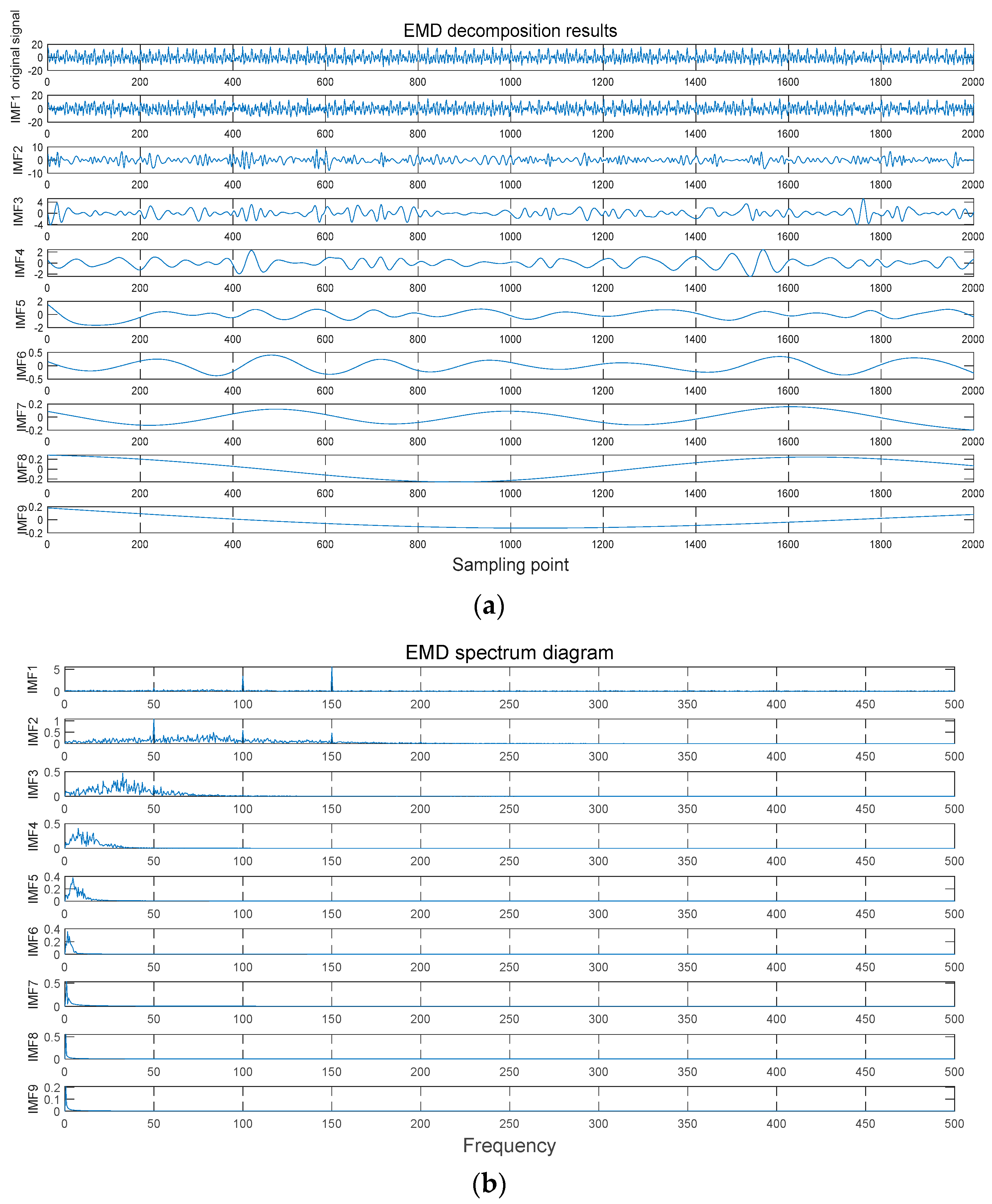
In order to compare the decomposition effect of VMD and EMD, as well as to illustrate the noise robustness of VMD, a noise-containing fault signal is decomposed using VMD and EMD, by giving a noise-containing fault signal in which the number of modes in the parameters of VMD is K = 4, α = 2000, and the sampling frequency is 1000 Hz. The decomposition diagrams of the EMD in the time and frequency domains are shown in Figure 2, and those of VMD in the time and frequency domains are shown in Figure 3.

From Figure 2 and Figure 3:

(1)

The low-frequency component of the VMD decomposition can better express the overall trend of the original signal waveform than the EMD decomposition;

(2)

The number of nine IMF components of EMD decomposition in Figure 2 cannot be set artificially, while VMD decomposition can be set according to one’s needs;

(3)

In the figure, the spectrum of EMD’s spectrogram spectrum is more blended, there is the phenomenon of mode aliasing, and the decomposition effect is poor, while the spectrum of VMD’s spectrogram spectrum is more clear, and there is the endpoint effect in the EMD’s IMF waveform diagram;

(4)

The VMD decomposition has good noise robustness and better representation of spectral features in spectrograms.

From the above analysis, it can be seen that the decomposition effect of VMD algorithm is better than EMD algorithm. So, in this paper, we choose the combination of VMD and HHT algorithms to process the fault traveling wave signals of transmission lines.

3.3. NGO Optimization VMD

VMD has the advantages of high accuracy, wide applicability, and strong anti-interference in fault location, but the decomposition effect of VMD is mainly related to the number of modal decomposition layers K and the penalty factor α. Therefore, this paper proposes to use the NGO algorithm to seek the optimization of the two key parameters of VMD, in order to improve the decomposition effect of VMD, and the minimum envelope entropy is used as the objective function of the optimization. Envelope entropy can reflect the sparsity degree of the VMD decomposition signal, if the current signal is decomposed by the VMD to get more IMF component noise, the smaller the sparsity degree of the reaction signal, the larger the envelope entropy, and vice versa [21,22].

Therefore, the whole optimization process is to find the global minimum envelope entropy and the corresponding K and α values. The envelope entropy is calculated as:

$$\left\{\begin{array}{l}{E}_p=-{\displaystyle \sum _{j=1}^N{e}_j\lg e_j}\\ e_j=\frac{a\left(j\right)}{{\displaystyle \sum _{j=1}^{N}a\left(j\right)}}\end{array}\right.$$

(28)

where $a\left(j\right)$ is the result obtained after Hilbert demodulation of the IMF component of the VMD decomposition, $e_j$ is the result obtained by normalizing $a\left(j\right)$.

With the iterative update of the parameter combination, different local optimal components will be generated, and each optimal component has a corresponding envelope entropy value, at this time, the IMF component with the smallest envelope entropy value is the optimal value of the parameter.

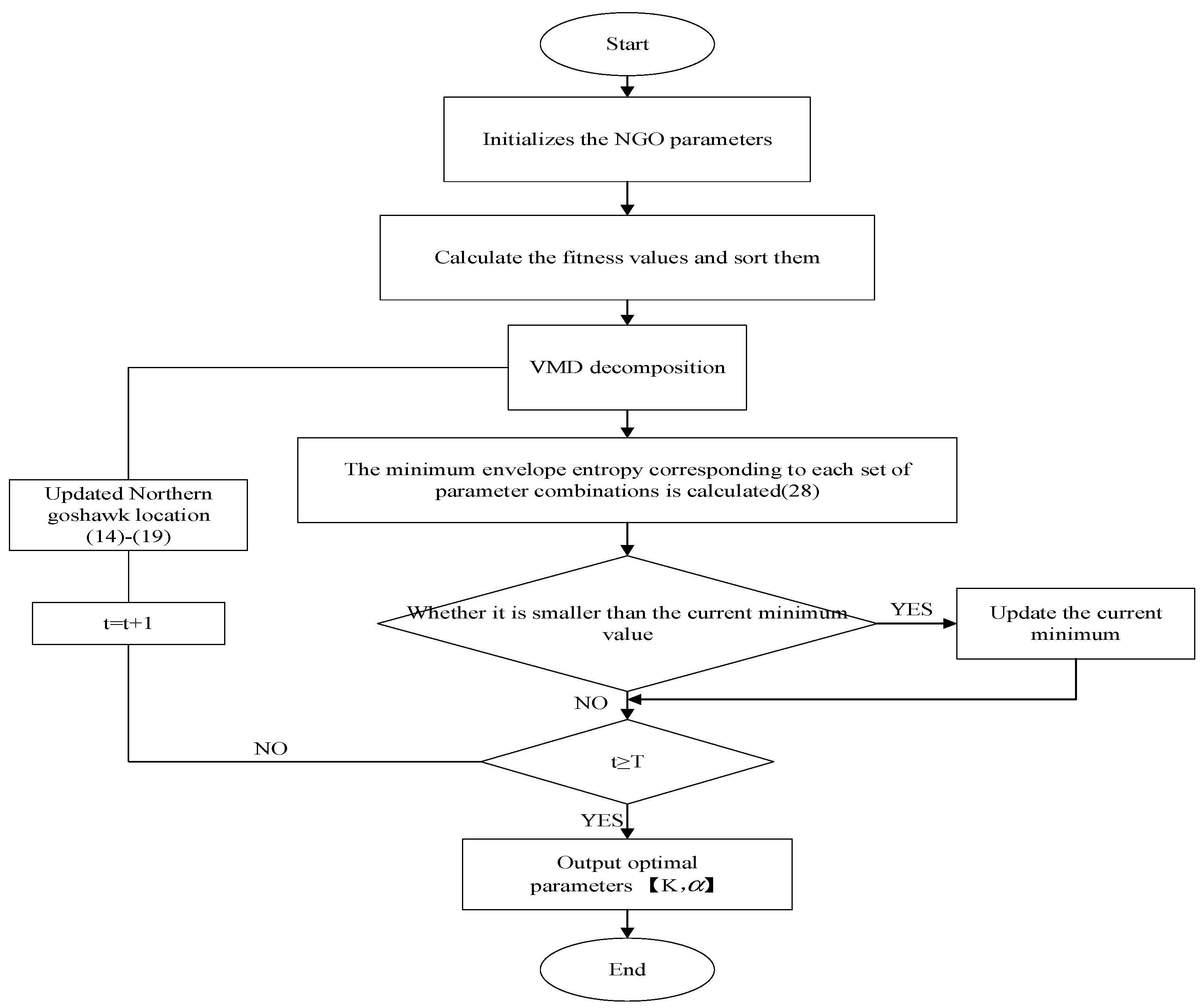
The implementation steps of the Northern Eagle optimization algorithm to optimize the variational modal decomposition are specified:

(1)

Initialize the parameters of the NGO algorithm, set the number of Northern Goshawk populations in the search process to 20, the maximum number of iterations to 15, and the range of values for the number of decomposition modal layers K values to $\left[1, 8\right]$, and the range of values for the penalty factor α to $\left[300, 2000\right]$;

(2)

Calculate and rank the size of individual adaptation value degrees;

(3)

The VMD decomposition is performed, and the objective function is chosen to be the minimum envelope entropy value $\min E_p$. This is computed by substituting pairs of K and α under different combinations each time, and updating the current best objective function value $\min E_p$;

(4)

Update the Northern Goshawk position according to Equations (14)–(19);

(5)

Determines whether to end the iteration. If $t\ge T$ then the iteration ends and the optimal parameter combination $\left[K, \alpha \right]$ is output, otherwise $t=t+1$ and the update continues.

Figure 4 illustrates the step-by-step flow of the NGO-VMD algorithm.

The optimal combination $\left[K, \alpha \right]$ after the optimization algorithm of the Northern Eagle optimization is $\left[6, 1200\right]$. To validate the decomposition capability of the NGO-VMD algorithm for signals, the NGO-VMD decomposition was performed on the given noisy fault signal mentioned in the previous section, and the decomposition waveforms are shown in Figure 5.

From Figure 5, the optimized VMD of NGO can divide the noise-containing signal into six layers by the frequency, i.e., the number of modal decomposition layers is six. Meanwhile, from the figure, the IMF1 component signal has a high degree of similarity to the waveform trend of the original signal of the fault and almost does not contain harmonic signals, so that the NOV-VMD algorithm has a very good decomposition ability of the faulty signals, and it still has a strong robustness to the noise. At the same time, the NGO-VMD algorithm can adaptively find the optimal value of the VMD parameters, avoiding the problem of determining the parameters due to subjective judgment.

3.4. Wave-Speed Independent Double-Ended Traveling Wave Localization Algorithm

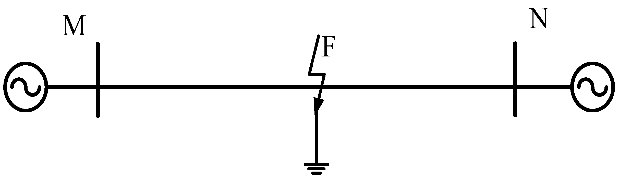
According to the difference in ranging principles, traveling wave fault ranging techniques can be categorized into single-ended traveling wave ranging techniques and double-ended traveling wave ranging techniques. The single-ended traveling wave ranging technique only requires the deployment of corresponding transformers at one end of the line, while the double-ended traveling wave ranging technique requires the installation of transformers at both ends of the line [23,24]. In this paper, the double-ended traveling wave fault location technique is used to calculate the fault distance by using the difference between the wave speed and time of the initial traveling wave of the fault arriving at each end, and its principle is shown in Figure 6.

The fault ranging formula for the double-ended traveling wave method is:

$$\left\{\begin{array}{l}{d}_M=\frac{L_{MN}+v\left(t_M-t_N\right)}{2}\\ d_N=\frac{L_{MN}+v\left(t_N-t_M\right)}{2}\end{array}\right.$$

(29)

where $L_{MN}$ is the distance of the line MN, $t_M$ and $t_N$ are the time when the initial wave head of the faulty traveling wave arrives at the M and N ends, respectively, and $v$ is the wave speed of the faulty traveling wave.

Equation (29) shows that fault localization is closely related to the actual length of the line, the traveling wave speed and the time when the traveling wave head reaches each end. Assuming that the line is faulted at the moment $t_0$, and $d_M^{\ast }$ and $d_N^{\ast }$ are the actual fault distance from the fault point F to the M and N ends, there are:

$$\left\{\begin{array}{l}{d}_M^{\ast }=\left(t_M-t_0\right)v\\ d_N^{\ast }=\left(t_N-t_0\right)v\end{array}\right.$$

(30)

Therefore, it can be obtained that the actual calculated distance of the line MN is:

$$L_{MN}^{\ast }=\left(t_M+t_N-2t_0\right)v$$

(31)

Assuming that the conductors to the same line are uniformly stretchable under the same external environment, the ratio of the actual length $L_{MN}^{\ast }$ of the line to the actual length $d_M^{\ast }$ of the faulted point F, to the end of M when the faulted point is close to the end of M, is approximately equal to the ratio of the length $L_{MN}$ of the end of MN to the ratio of the $d_M$ of the distance from the faulted point F to the end of M. Thus, there is:

$$\frac{L_{MN}}{d_M}=\frac{L_{MN}^{\ast }}{d_M^{\ast }}$$

(32)

Therefore, it can be obtained that the horizontal distance $d_M$ from the fault point F to the end of M is:

$$d_M=\frac{d_M^{\ast }}{L_{MN}^{\ast }}{L}_{MN}=\frac{\left(t_M-t_0\right)L_{MN}}{t_M+t_N-2t_0}$$

(33)

As can be seen from Equation (33), this method of ranging only needs to know the horizontal distance of the transmission line, the initial time of the fault occurrence, and the time data of the traveling wave arriving at the two ends of the line, and is no longer affected by the change of wave speed. In addition, the occurrence of time data in the formula of the method are all time differences, thus reducing the effect of errors caused by time desynchronization.

3.5. Fault Localization Steps

Establish the transmission line double-ended traveling wave ranging process with the following steps:

Step 1: Build the simulation model through MATLAB, set the fault location and fault circuit parameters, simulate the experiment, and extract the fault current traveling wave signal from the simulation system recording device.

Step 2: Perform phase mode transformation using the improved phase mode transformation matrix to decouple and obtain the current traveling wave line mode components.

Step 3: The current traveling wave line mode component is decomposed by VMD after NGO optimization to obtain the IMF component, and the Hilbert transform is performed on the IMF1 component to obtain its instantaneous frequency, and then extract the initial wavehead of the fault current traveling wave.

Step 4: The location of the fault point is calculated based on the time detected to the ends of M and N, and its substitution to the improved double-ended traveling wave ranging method formula, i.e., Equation (33).

4. Simulation Analysis

To verify the reliability of the method proposed in this paper, a simulation model of transmission line faults was constructed using MATLAB software (version R2022a), as shown in Figure 7.

The total length of the transmission line simulation model line MN is 100 km, the simulation model is a double-fed power supply system, in which the voltage level is 220 kV, the frequency is 50 Hz, and the sampling frequency is 1 MHz. The positive sequence and zero sequence parameters of the transmission line are shown in

Table 2. Transmission line positive sequence and zero sequence parameter table.

Phase Sequence	$\mathit{R}$ $\mathbf{\Omega }/\mathbf{km}$	$\mathit{L}$ $\mathbf{mH}/\mathbf{km}$	$\mathit{C}$ $\mathbf{\mu }\mathbf{F}/\mathbf{km}$
Positive sequence	0.0208	0.8984	0.0129
Zero sequence	0.1148	2.2886	0.0084

.

To ascertain the effectiveness of the fault traveling wave feature extraction algorithm and fault location method proposed herein across diverse fault scenarios, comprehensive simulation analyses were performed within a transmission line simulation framework. These analyses built on the fault location procedures outlined in the preceding section, incorporating a range of fault conditions to evaluate the methods’ effectiveness.

4.1. Simulation Analysis at Different Fault Locations

To validate the applicability of the fault location method proposed in this paper in different fault locations, different fault locations are set up for simulation analysis.

Firstly, the fault is set at a distance of 20 km from the M-terminal, the transition resistance is 50 Ω, the initial phase angle of the fault is 0°, and the A-phase grounded short-circuit fault occurs; the fault occurs at 0.016 s, and the whole simulation process lasts for 0.05 s. After the fault occurs, the waveforms of the three-phase traveling currents of the two measurement points of the M point and the N point are shown in Figure 8.

To obtain the transient quantities of the current traveling wave signals, an improved phase-to-mode transformation matrix is utilized for phase-mode transformation, and the extracted current traveling wave line mode component is used as the analysis object for the fault traveling wave signals. The waveforms of the current traveling wave line mode components at measurement points M and N are shown in Figure 9.

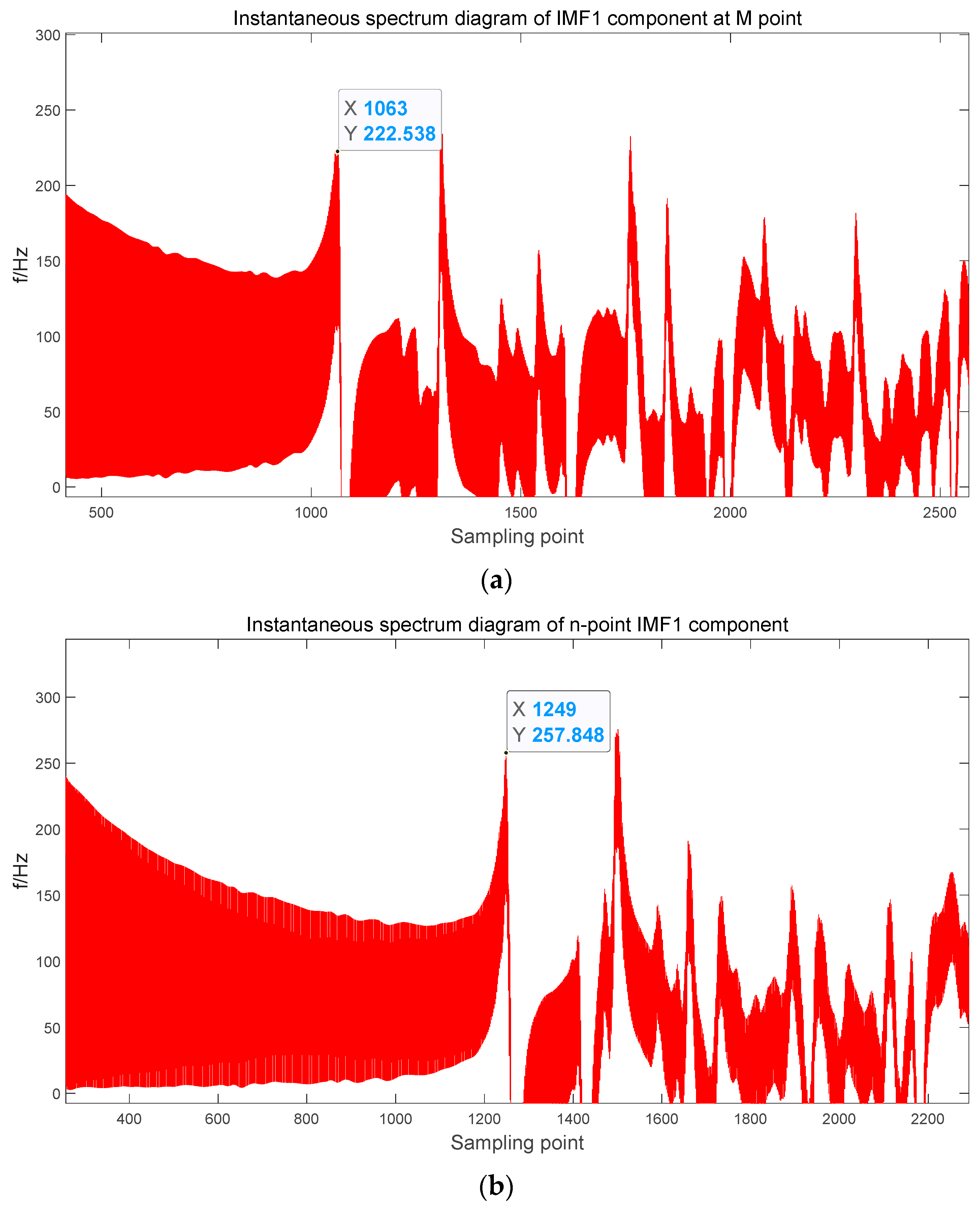
Using the NGO-VMD-HHT algorithm to decompose the line mode component of the fault current traveling wave and extract the time of the initial traveling wave head of the fault arriving at the detection points at the M and N ends, then using the improved formula of the double-ended traveling wave ranging method, the distance of the fault is accurately calculated to achieve the purpose of fault location. Since the fault occurrence time is 0.016 s in the simulation model, the 15,000th sampling point to the 25,000th sampling point, 10,000 sampling points, are taken for the experiment, i.e., the experimental data from the 0.015 s to the 0.025 s are taken. Among them, the NGO-VMD-HHT decomposition signals of point M and point N are shown in Figure 10.

From Figure 10, it can be obtained that the waveform trends of the amplitude of IMF1 and line mode components are most similar, and by applying the Hilbert transform, the instantaneous spectrogram of the IMF1 component can be obtained. When analyzing the instantaneous spectrogram of the MF1 component, it can be found that the first frequency mutation point corresponds to the instant when the traveling wave arrives for the first time, so by extracting the data of the first mutation point, we can obtain the time when the initial traveling wave arrives at the two different measurement points of M and N. The data detection diagram of the first mutation point of the instantaneous spectrogram of the IMF1 component at the M point and the N point is shown in Figure 11.

Since the time period taken is from the 15,000th sample point to the 25,000th sample point, i.e., 0.015 s to 0.016 s, t = 0.015 + sample point/${10}^6$ in s. Hence, $t_M=0.01606 1\mathrm{s}$, $t_N=0.016243 \mathrm{s}$.

Substituting $L_{MN}=100 \mathrm{km}$, $t_M=0.01606 1\mathrm{s}$, $t_N=0.016243 \mathrm{s}$, and $t_0=0.016 \mathrm{s}$ into Equation (33), yields $d_M$ = 20.066 km and the relative error is calculated, which is given by Equation:

$${\epsilon }_r\%=\frac{\left|\mathrm{Fault} \mathrm{distance}-\mathrm{Ranging} \mathrm{results}\right|}{\mathrm{Total} \mathrm{line} \mathrm{length}}\times 100\%$$

(34)

According to Equation (34), the relative error is 0.066%.

Similarly, the A-phase short-circuit fault is simulated at different distances of 40, 55, and 70 km from the M-terminal, and the results are shown in

Table 3. Fault localization results at different fault locations.

Fault Location/km	Fault Localization/km	$\mathbf{Error} \mathbf{(}\mathit{\epsilon }\mathbf{/}\mathbf{km}\mathbf{)}$	$\mathbf{Relative} \mathbf{Error} \mathbf{(}{\mathit{\epsilon }}_{\mathit{r}}\mathbf{\%}\mathbf{)}$
20	20.066	0.066	0.066
40	39.937	0.063	0.063
55	55.031	0.031	0.031
70	69.937	0.063	0.063

.

As shown in Table 3, the fault location method based on the NGO-VMD-HHT algorithm has a relative error of less than 1% at different fault positions, meeting the requirements for precise fault location and being suitable for practical engineering applications.

4.2. Simulation Analysis with Different Transition Resistances

To validate the robust applicability of the fault location method proposed in this paper under various transition resistance conditions, this section conducts simulation experiments on the transmission line model at the same fault location. All other conditions remain constant, with only the fault transition resistance being altered.

Different transition resistances are set in MATLAB: 50 Ω, 100 Ω, and 200 Ω. With different transition resistances, the waveforms of the line mode components at points M and N are shown in Figure 12, for example, if the fault occurs at a distance of 20 km from end M. The waveforms of the line mode components at point M and N are shown in Figure 12.

As illustrated in Figure 12, with the increase of transition resistance, the amplitude of the line mode component decreases. However, the mutation point of the line mode component and the trend of waveform change are not affected by the variation in transition resistance. Using the fault location method based on NGO-VMD-HHT, fault location results under different transition resistances can be obtained, as shown in

Table 4. Fault localization results for four fault locations with different transition resistances.

Fault Location/km	Transition Resistance/Ω	Fault Localization/km	$\mathbf{Error} \mathbf{(}\mathit{\epsilon }\mathbf{/}\mathbf{km}\mathbf{)}$	$\mathbf{Relative} \mathbf{Error} \mathbf{(}{\mathit{\epsilon }}_{\mathit{r}}\mathbf{\%}\mathbf{)}$
20	50	20.066	0.066	0.066
	100	20.066	0.066	0.066
	200	20.066	0.066	0.066
40	50	39.937	0.063	0.063
	100	39.937	0.063	0.063
	200	39.937	0.063	0.063
55	50	55.031	0.031	0.031
	100	55.031	0.031	0.031
	200	55.031	0.031	0.031
70	50	69.937	0.063	0.063
	100	69.937	0.063	0.063
	200	69.937	0.063	0.063

.

Table 4 indicates that the double-ended traveling wave fault location method proposed in this paper, based on the NGO-VMD-HHT algorithm, is not affected by different transition resistances. It can still achieve precise location under various transition resistances, with the relative error of fault ranging within 1%, meeting the requirements for accurate ranging.

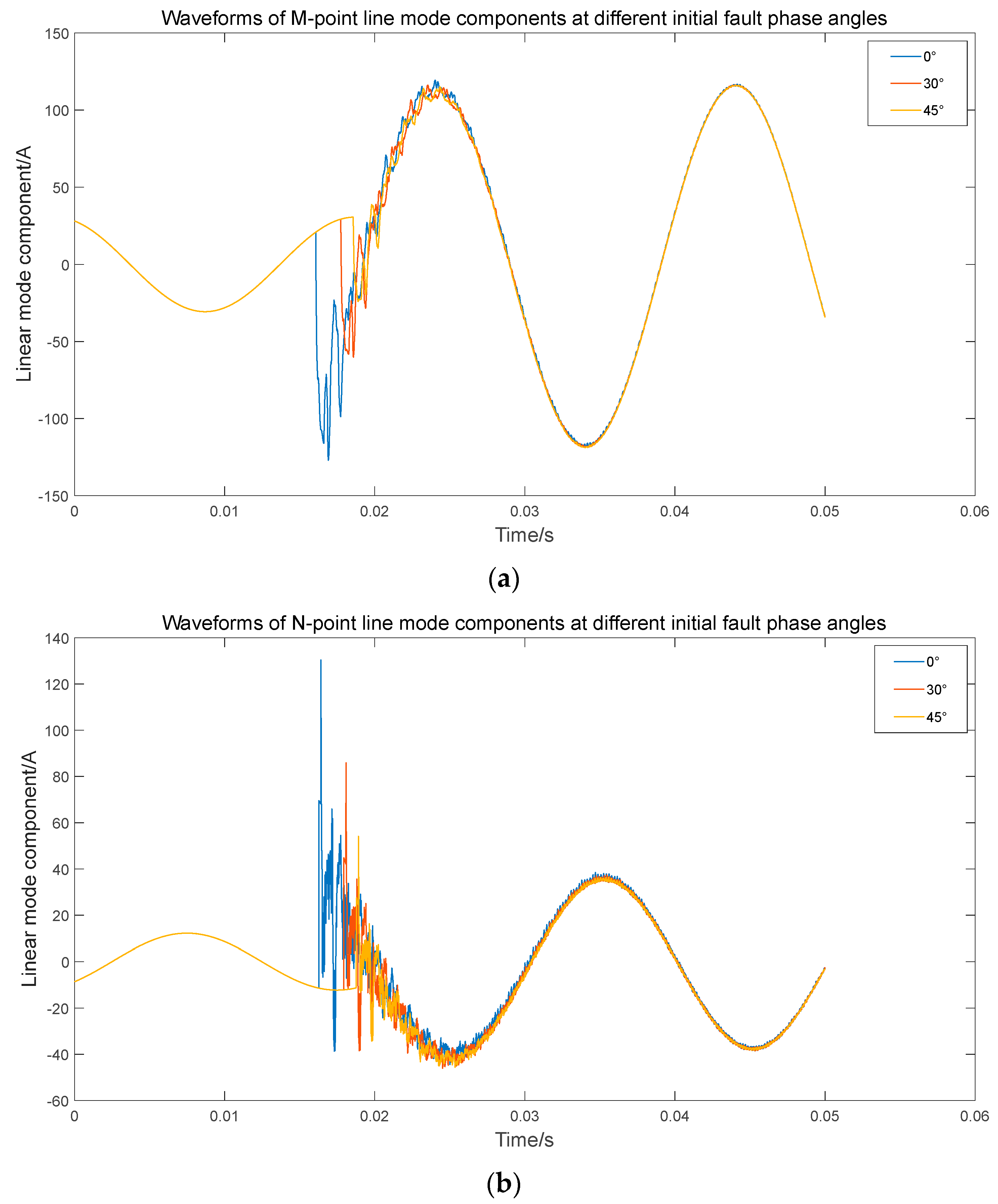
4.3. Simulation Analysis under Different Fault Initial Phase Angles

To validate the applicability of the fault location method proposed in this paper under different initial fault phase angles, this section conducted simulation experiments on the transmission line model with the same fault location but varying initial fault phase angles. All other parameters were kept constant, with the transition resistance maintained at 50 Ω.

The fault initial phase angles were set to 0°, 30°, and 45°, taking the fault occurrence at a distance of 20 km from terminal M as an example. The waveforms of the line mode components at points M and N are shown in Figure 13.

From Figure 13, with the change of the fault initial phase angle, there is a slight difference in the amplitude of the line mode component waveforms at the same point between point M and point N. However, the change trend of the waveforms of the line mode components is not affected by the fault initial phase angle. Using the fault localization method based on NGO-VMD-HHT, the fault localization results under different fault initial phase angles can be obtained. The fault localization results of four fault locations under different fault initial phase angles are shown in

Table 5. Fault localization results of four fault locations under different fault initial phase angles.

Fault Location/km	Fault Initial Phase Angle/°	Fault Localization/km	$\mathbf{Error} \mathbf{(}\mathit{\epsilon }\mathbf{/}\mathbf{km}\mathbf{)}$	$\mathbf{Relative} \mathbf{Error} \mathbf{(}{\mathit{\epsilon }}_{\mathit{r}}\mathbf{\%}\mathbf{)}$
20	0	20.066	0.066	0.066
	30	20.071	0.071	0.071
	45	20.073	0.073	0.073
40	0	39.937	0.063	0.063
	30	40.066	0.066	0.066
	45	39.933	0.067	0.067
55	0	55.031	0.031	0.031
	30	54.952	0.048	0.048
	45	54.984	0.016	0.016
70	0	69.937	0.063	0.063
	30	70.096	0.096	0.096
	45	70.033	0.033	0.033

.

Table 5 shows that the double-ended traveling wave fault localization method, based on the NGO-VMD-HHT algorithm proposed in this paper, can still locate the faults accurately under different initial phase angles, and the relative errors of fault ranging are all within 1%, which meets the demand of accurate ranging.

4.4. Simulation Analysis with Different Analysis Methods

To further validate the accuracy of the NGO-VMD-HHT fault signal extraction algorithm proposed in this paper, a comparative analysis was conducted with the fault results obtained using the VMD-HHT algorithm without NGO optimization and the wavelet transform algorithm. For the VMD, the parameters were set to K = 4 and α = 2000; for the wavelet transform, the db5 wavelet basis function was used with a decomposition scale parameter of three. At the same time, the transition resistance is kept at 50 Ω, the initial phase angle of the fault is kept at 0°, and all other experimental parameters are kept unchanged. Taking the distance as an example, the fault occurs at 20 km from the M end, the simulation results of the wavelet transform algorithm are shown in Figure 14, and the simulation results of the VMD-HHT algorithm are shown in Figure 15.

From Figure 14 and the relationship between time and sampling point t = 0.015 + sampling point/${10}^6$ in s, it can be obtained that at this point $t_M$ = 0.016072 s and $t_N$ = 0.016275 s.

Substituting $L_{MN}=100 \mathrm{km}$, $t_M=0.016072 \mathrm{s}$, $t_N=0.016275 \mathrm{s}$, into Equation (33), yields $d_M$ = 20.749 km and substituting into Equation (34) % = 0.749% relative error.

From Figure 15 and the relationship between time and sampling point t = 0.015 + sampling point/${10}^6$ in s, it can be obtained that at this point $t_M$ = 0.016063 s and $t_N$ = 0.016249 s.

Substituting $L_{MN}=100 \mathrm{km}$, $t_M=0.016063 \mathrm{s}$, $t_N=0.016249 \mathrm{s}$, $t_0=0.016 \mathrm{s}$ into Equation (33), yields = 20.192 km and substituting into Equation (34) ${\epsilon }_r$% = 0.192% relative error.

Similarly, fault localization is carried out at different fault distances using the three analysis methods of NGO-VMD-HHT, VMD-HHT, and wavelet transform, and the simulation results of fault localization at four fault locations under different analysis methods are shown in

Table 6. Fault localization results of four fault locations under different analysis methods.

Fault Location/km	Algorithm Name	Fault Localization/km	Error $\mathbf{(}\mathit{\epsilon }\mathbf{/}\mathrm{km}\mathbf{)}$	Relative Error $\mathbf{(}{\mathit{\epsilon }}_{\mathit{r}}\mathbf{\%}\mathbf{)}$
20	Wavelet transform	20.749	0.749	0.749
	VMD-HHT	20.192	0.192	0.192
	NGO-VMD-HHT	20.066	0.066	0.066
40	Wavelet transform	39.706	0.294	0.294
	VMD-HHT	39.815	0.185	0.185
	NGO-VMD-HHT	39.937	0.063	0.063
55	Wavelet transform	54.519	0.481	0.481
	VMD-HHT	55.183	0.183	0.183
	NGO-VMD-HHT	55.031	0.031	0.031
70	Wavelet transform	70.317	0.317	0.317
	VMD-HHT	70.245	0.245	0.245
	NGO-VMD-HHT	69.937	0.063	0.063

below.

From Table 6, it can be seen that the relative error in fault localization using the improved double-ended traveling wave method, based on the traditional algorithm of wavelet transform and the VMD-HHT algorithm, is higher than that of the NGO-VMD-HHT algorithm proposed in this paper across different fault locations.

5. Conclusions

(1)

Considering that the VMD decomposition outcome is heavily influenced by the number of modal components K and the penalty factor α, this paper suggests employing the NGO algorithm to optimize these parameters, thereby ensuring a more rational selection of K and α;

(2)

In this paper, an improved double-ended traveling wave method without counting the wave speed is derived, and the algorithm does not have to consider the influence of the reflected wave of the traveling wave, which improves the accuracy of fault localization;

(3)

In this paper, the dual power supply network model of the transmission line is built in the simulation software, and four fault locations are selected to set up single-phase grounded short-circuit faults. The simulation shows that the ranging results of the NGO-VMD-HHT algorithm have higher accuracy than those of the traditional wavelet transform and the VMD-HHT algorithm in fault localization, and the method can accurately locate faults with different transition resistances and different initial phase angles of faults, and the relative errors are within 1%, which meets the requirements of the actual engineering ranging accuracy;

(4)

The fault localization method proposed in this paper combines the improved double-ended traveling wave method and the newly introduced NGO-VMD-HHT algorithm, which effectively solves the difficulties related to identifying faulty wave signals and the differences in wave propagation speeds. This innovative method is promising for practical engineering applications.

References

- Sun, Q.Z. Operation status and lightning protection of transmission lines in China. Electr. Technol. Econ. 2022, 28, 146–149. [Google Scholar]
- Chen, J.H.; Zhang, Q.; Feng, W.X.; Fang, Y.H. Lightning localization system and lightning monitoring network for power grid in China. High Volt. Technol. 2008, 3, 425–431. [Google Scholar]
- Cai, D.Y. Research on Fault Localization of Transmission Network Based on Improved Impedance Method. Ph.D. Thesis, Chongqing University of Posts and Telecommunications, Chongqing, China, 2021. [Google Scholar]
- Wang, B.; Dong, X.Z.; Bo, Z.Q.; Andrew, K. Ranging of single-phase ground faults by single-end impedance method for extra-high voltage long lines. Power Syst. Autom. 2008, 32, 25–29. [Google Scholar]
- Deng, H.; Geng, L. Analysis of the impedance measurement of transmission lines with two-phase short circuit. In Proceedings of the 2011 International Conference on Consumer Electronics, Communications and Networks (CECNet), Xianning, China, 16–18 April 2011; IEEE: New York, NY, USA, 2011; pp. 1063–1066. [Google Scholar]
- Sardar, A.; Husnine, S.M.; Rizvi, S.T.R.; Younis, M.; Ali, K. Multiple travelling wave solutions for electrical transmission line model. Nonlinear Dyn. 2015, 82, 1317–1324. [Google Scholar] [CrossRef]
- Wen, Z.; Luo, S.X.; Liu, F.; Guo, J.K.; Zheng, L.H. Traveling wave localization of 220 kV transmission line faults in hydropower stations. Hydropower Energy Sci. 2023, 41, 198–201+166. [Google Scholar]
- Tao, Y.; Fan, K.; Wang, K.B.; Sun, Z.W. Single-end traveling wave ranging fault localization of transmission lines based on spatio-temporal full data. Manuf. Autom. 2023, 45, 39–43. [Google Scholar]
- Liu, J. Research on fault localization method of ultra-high voltage transmission line based on improved double-ended traveling wave method. Northeast. Electr. Power Technol. 2023, 44, 11–15. [Google Scholar]
- Yang, S.; Xu, P.K. Traveling wave fault localization of ground cable overhead hybrid lines based on time linear fitting. J. Chongqing Gongshang Univ. (Nat. Sci. Ed.) 2024, 1–10. [Google Scholar]
- Wu, J.; Xue, Y.S.; Shan, C.F.; Tan, Q.S. Research on fault location in distribution network based on improved artificial fish swarm optimization algorithm. J. Electr. Power Sci. Technol. 2023, 38, 40–47. [Google Scholar]
- Zhang, L.; Zhang, S.D.; Jia, H.; Zhao, M.Q.; Zhao, N.; Li, D. Fault zone localization in distribution network based on improved whale algorithm. Zhejiang Electr. Power 2022, 41, 63–70. [Google Scholar]
- Li, B.W.; Ma, B.J.; Kong, D.J.; Zhao, H.L. Application of simulated annealing-Newton method in fault localization of high-voltage transmission lines. Electr. Autom. 2019, 41, 64–66. [Google Scholar]
- Lin, J.Y. Research on Fault Localization Based on Synchronous Phase Measurement Device in Distribution Network. Master’s Thesis, Huazhong University of Science and Technology, Wuhan, China, 2022. [Google Scholar]
- Ding, X.P.; Lin, Y.; Yu, H. Research on cable fault localization based on improved HHT. Electromechanical Inf. 2022, 20, 82–85. [Google Scholar]
- Puliafito, V.; Vergur, S.; Carpentieri, M. Fourier, Wavelet, and Hilbert-Huang Transforms for Studying Electrical Users in the Time and Frequency Domain. Energies 2017, 10, 188. [Google Scholar] [CrossRef]
- Lu, Z.Y.; Lu, Y.M.; Xia, Z.W.; Huang, X.Y. Speech signal denoising method based on variational modal decomposition and wavelet analysis. Mod. Electron. Technol. 2018, 41, 47–51. [Google Scholar]
- Jiang, Y.; Chen, L.; Zeng, W.; Xin, Y. Adaptive Weighted VMD-WPEE Method of Power-Electronic-Circuit Multiple-Parameter-Faults Diagnosis. IEEE J. Emerg. Sel. Top. Power Electron. 2019, 8, 3878–3890. [Google Scholar] [CrossRef]
- Dehghani, M.; Hubálovský, Š.; Trojovský, P. Northern goshawk optimization: A new swarm-based algorithm for solving optimization problems. IEEE Access 2021, 9, 162059–162080. [Google Scholar] [CrossRef]
- He, J.H.; Zhang, B.; Fan, Y.; Ou, Z.J. Application of decoupling transformation in power system transient protection. J. Beijing Jiaotong Univ. 2006, 5, 101–104. [Google Scholar]
- Zang, Y.; Lv, G.Y.; Chu, C.J.; Xu, X.D.; Cao, B.; Zhang, X.Y. Voltage-drop source localization method based on entropy weight of current-voltage wavelet envelope. J. Nanjing Eng. Coll. (Nat. Sci. Ed.) 2020, 18, 8–13. [Google Scholar]
- Qin, Q.D.; Huang, Z.R.; Zhou, Z.H.; Fan, B.; Yu, L.A. Research on two-layer decomposition influenza prediction model based on envelope entropy. Syst. Eng. Theory Pract. 2023, 43, 3505–3519. [Google Scholar]
- Chai, P.; Zhou, H.; Zhang, Y.; Zhao, W.J.; Yang, X.; Zhou, M.; Li, M.Z. Improvement of short-circuit fault localization in cable lines based on double-ended traveling wave method. China Electr. Power 2020, 53, 168–174. [Google Scholar]
- Zhang, K.; Zhu, Y.L.; Ma, C.X.; Cao, Y.Q.; Liu, S. A new method of traveling wave ranging for transmission lines based on optimizing traveling wave speed. J. North China Electr. Power Univ. (Nat. Sci. Ed.) 2018, 45, 34–40. [Google Scholar]
Figure 1.
Equivalent network for electromagnetic coupling of three-phase systems.
Figure 2.
EMD time-domain and frequency-domain decomposition diagram. (a) EMD time-domain decomposition diagram. (b) EMD frequency-domain decomposition diagram.
Figure 3.
VMD time-domain and frequency-domain decomposition diagram. (a) VMD time-domain decomposition diagram. (b) VMD frequency-domain decomposition diagram.
Figure 4.
NGO-VMD algorithm flowchart.
Figure 5.
NGO-VMD exploded view.
Figure 6.
Fault traveling wave transmission diagram.
Figure 7.
Transmission line simulation model.
Figure 8.
Three-phase current waveform diagram of M and N measuring points. (a) M point three-phase current wave shape. (b) N point three-phase current wave shape.
Figure 9.
Waveform diagram of the line mode component of the current wave at the M and N ends of the measuring point. (a) Waveform diagram of the line mode component of the M-point current wave. (b) Waveform diagram of the line mode component of the N-point current wave.
Figure 10.
Signal decomposition diagram of M and N terminals of measurement points. (a) IMF components at the M end of the measurement point. (b) IMF components at the N end of the measurement point.
Figure 11.
Instantaneous spectrum diagram of IMF1 component of M, N point. The first mutation point data detection diagram. (a) Instantaneous spectrum diagram of IMF1 component of M point. The first mutation point data detection diagram. (b) Instantaneous spectrum diagram of IMF1 component of N point. The first mutation point data detection diagram.
Figure 12.
Waveforms of linear mode components of different transition resistors at M and N points. (a) Waveforms of linear mode components of different transition resistances at point M. (b) Waveforms of linear mode components of different transition resistances at point N.
Figure 13.
Waveforms of initial phase angular line mode components for different faults at M and N points. (a) Waveforms of initial phase Angle line mode components for different faults at point M. (b) Waveforms of initial phase angular line mode components for N-point different faults.
Figure 14.
Simulation results of wavelet transform algorithm. (a) M-point electrical wave mode component wavelet transform. (b) N-point electrical wave mode component wavelet transform.
Figure 15.
Simulation results of VMD-HHT algorithm. (a) Instantaneous spectrum diagram of M-point IMF1 component first mutation point data detection diagram. (b) Instantaneous spectrum diagram of N-point IMF1 component first mutation point data detection diagram.