Investigating the Effect of Large Wind Farms on Energy in the Atmosphere

Abstract

This study presents a parameterization of the interaction between wind turbines and the atmosphere and estimates the global and regional atmospheric energy losses due to such interactions. The parameterization is based on the Blade Element Momentum theory, which calculates forces on turbine blades. Should wind supply the world’s energy needs, this parameterization estimates energy loss in the lowest 1 km of the atmosphere to be ~0.007%. This is an order of magnitude smaller than atmospheric energy loss from aerosol pollution and urbanization, and orders of magnitude less than the energy added to the atmosphere from doubling CO₂. Also, the net heat added to the environment due to wind dissipation is much less than that added by thermal plants that the turbines displace.

1. Introduction

Wind Energy is currently one of the fastest growing new electric power sources. With this speed of development, it is important to evaluate the impact of wind farms on the environment. Aside from the issues of aesthetics [1,2,3], which is subjective, and effects on wildlife [4,5,6,7], which may be smaller than effects of conventional energy sources that wind displaces [7], another concern raised with respect to wind energy is the feedback of large wind farms to weather and climate. Knowing the effects of wind farms on the wind flow will help in site selection and in determining the best layout required to optimize power capture by wind farms.

A number of modeling studies have examined the feedback of wind turbines or farms to weather or climate at coarse spatial resolution. A common approach in such models has been to modify surface drag to simulate the effect of wind farms [8,9]. Results have varied from suggesting that a large deployment of wind farms would cause local temperatures to rise by a few degrees [9], with negligible changes in global mean temperatures, to possibly changing weather and climate features [10]. Another parameterization simulated wind turbine effects by adding an elevated sink of resolved kinetic energy (RKE), and a source of turbulent kinetic energy (TKE) [11]. That study found that the increased near surface turbulence due to a wind farm affected local near-surface heat and vapor fluxes. The turbulence behind the rotors increased mixing and sensible heat fluxes from the atmosphere to the ground while increasing the vapor flux from the ground to the atmosphere. A more recent study used a mesoscale model to examine wind farm effects [12]. They parameterized the wind farms by formulating a drag coefficient based on the thrust coefficients of a wind turbine, as the thrust coefficient is a measure of the force the turbine exerts on the wind flow. The study assumed that part of the energy lost from the wind due to drag is extracted as electric power, and the remaining energy is added to the turbulent kinetic energy of the flow. Their results showed increased mixing in the boundary layer, leading to increased surface temperatures.

2. Blade Element Momentum Model

Typically used for blade design, the BEM theory was formulated by Glauert [13,14] and gives both the force in the axial direction, or the direction parallel to the rotor’s axis of rotation, and the tangential direction, or the direction tangent to the rotor radius. The axial force is called the thrust and the tangential force is the force related to the torque.

The BEM theory assumes that the turbine rotor can be divided into non-interacting annular rings (Figure 1). The forces on these rings are analyzed using a combination of momentum theory and blade element theory. Momentum theory gives the thrust force, T, from the pressure difference across that annular ring—the pressure difference is driven by the loss of axial momentum of the incoming flow as energy is extracted at the rotor. The torque, Q, is computed as the change in angular momentum imparted by the rotating blades. More information about T and Q are gleaned from blade element theory, where these annular rings divide the blades into elements whose cross-sections resemble an airfoil. Lift and drag forces on the blade elements are estimated using 2D airfoil theory. The forces at each blade element, dT and dQ, are then derived as a combination of the lift and drag experienced by that blade element. Integrating dT and dQ over the whole blade gives the total thrust and torque experienced by the rotor. The resulting T acts as a pressure drag, slowing the wind down, while the spinning blades apply Q onto the air flowing through the rotor, generating rotation in the wake.

This analysis is based on the assumptions that the incoming wind speed is steady and perfectly perpendicular to the rotor plane, and that there is no interaction between annular rings—i.e., 3D effects are neglected. Although in reality, a steady, perpendicular incoming wind rarely occurs in the field [15], the error introduced by this assumption is not so large as it could be since modern turbines are built to yaw in order to face the wind. The errors from neglecting 3D effects however, are more problematic since there is reduced lift near the tip of the blade [16] that is not simulated by this 2D analysis. Another limitation is that momentum theory breaks down at low wind speed. At low wind speed, the wake becomes turbulent and, instead of energy being extracted at the rotor, energy goes into recirculating the wake. In order to correct these limitations and errors, empirical parameterizations need to be added to the basic theory, but even with these modifications, extracted power is still currently underestimated at low wind speed [17]. Despite this, BEM results are generally acceptable, especially when the wind is relatively steady and uniform. Since it is also the simplest and most straightforward to implement, this model is the model used most by the wind industry today. A number of turbine studies that use BEM include References 18 and 19.

Figure 1. Annular rings on a turbine rotor.

Figure 1. Annular rings on a turbine rotor.

Although there are other, more detailed methods of describing the flow around turbine blades—such as the vortex wake method [20,21] and computational fluid dynamics (CFD) methods [22,23]—the BEM method was chosen because it is relatively straightforward to implement and computationally inexpensive. Since the BEM model is applied here to estimating the effect of wind turbines on the wind flow for the purpose of building a parameterization, the level of detail provided by these other methods is not required. The version of the BEM model that we implemented is described in Reference 24.

To illustrate the application of the BEM method to this study, the BEM model results are compared with data for three turbines. Since thrust and torque data on wind turbines are not readily available, the torque calculate by the model is converted into power and compared with the power curves associated with the turbine test cases. The power is calculated as the product of the torque and the rotor’s angular velocity, Ω:

$$P=\mathrm{\Omega }{\displaystyle \int dQ}$$

(1)

As the power is a function of the aerodynamic forces applied to the turbine rotor, a comparison gives a good indication of how well the model is simulating the aerodynamic system.

3. Power Curve Comparisons

The characteristics of three different turbines were input into the BEM model and power curves were generated as a function of incoming wind speed, V₀, for all three turbines. The model-generated power curves were compared with the expected power output of these turbines.

The first test case was the turbine used in Phase VI of the NASA/NREL Unsteady Aerodynamics Experiment (UAE). The National Renewable Energy Laboratory (NREL), together with NASA-Ames, conducted wind tunnel studies on a wind turbine to develop a database of aerodynamic and flow parameters. These parameters were used in a blind comparison between different wind turbine modelers. This experiment, called the Unsteady Aerodynamics Experiment (UAE), aimed to test the validity and range of applicability of the different turbine models involved, as well as to determine areas of improvement [18]. The second turbine used for validation had a blade designed by LM Glasfiber (LMG). The blade and power curve data were provided by Peter Hansen from LM Glasfiber (pers. comm.). The third turbine was a 2 MW experimental wind turbine in Tjaereborg, Denmark. For this turbine, only the power generated from the cut-in wind speed (5 m/s) to 14 m/s (when rated power is reached) is used for comparison. This is because this particular turbine uses variable blade pitching for power control, and the BEM model cannot currently simulate this feature. The characteristics of the different turbines are summarized in Table 1.

Table 1. Summary of turbine properties for model validation.

Turbine type	No. of blades	Blade radius (m)	Rotation speed (rpm)	Rated Power (kW)	Cut-in wind speed (m/s)
NREL UAE	2	5	71.63	19.8	6
LMG	3	29	19	1,500	5
Tjaereborg	3	30	22	2,000	5

Table 1. Summary of turbine properties for model validation.

Turbine type	No. of blades	Blade radius (m)	Rotation speed (rpm)	Rated Power (kW)	Cut-in wind speed (m/s)
NREL UAE	2	5	71.63	19.8	6
LMG	3	29	19	1,500	5
Tjaereborg	3	30	22	2,000	5

Figure 2 shows how the two power curves compare for the NREL turbine. The data for the NREL turbine was taken from Reference 25. The agreement is best at low to medium wind speeds, but at higher wind speeds, the model over-predicts the power. This may be because the model does not include a way to handle stall. Stall occurs when the flow separates from the blade, which increases the drag and lift. This is typically how fixed-pitch turbines regulate their power generation and keep it at the rated value. The rated power is generally reached at about 12–15 m/s, depending on the turbine, so stall acts to decrease power generation after that wind speed is reached. This phenomenon needs to be modeled differently once the rated power is reached but this is not dealt with here.

Figure 2. NREL power comparison as a function of incoming wind speed, V₀. The gray lines indicate the range of wind speeds that are relevant for wind energy production.

Figure 2. NREL power comparison as a function of incoming wind speed, V₀. The gray lines indicate the range of wind speeds that are relevant for wind energy production.

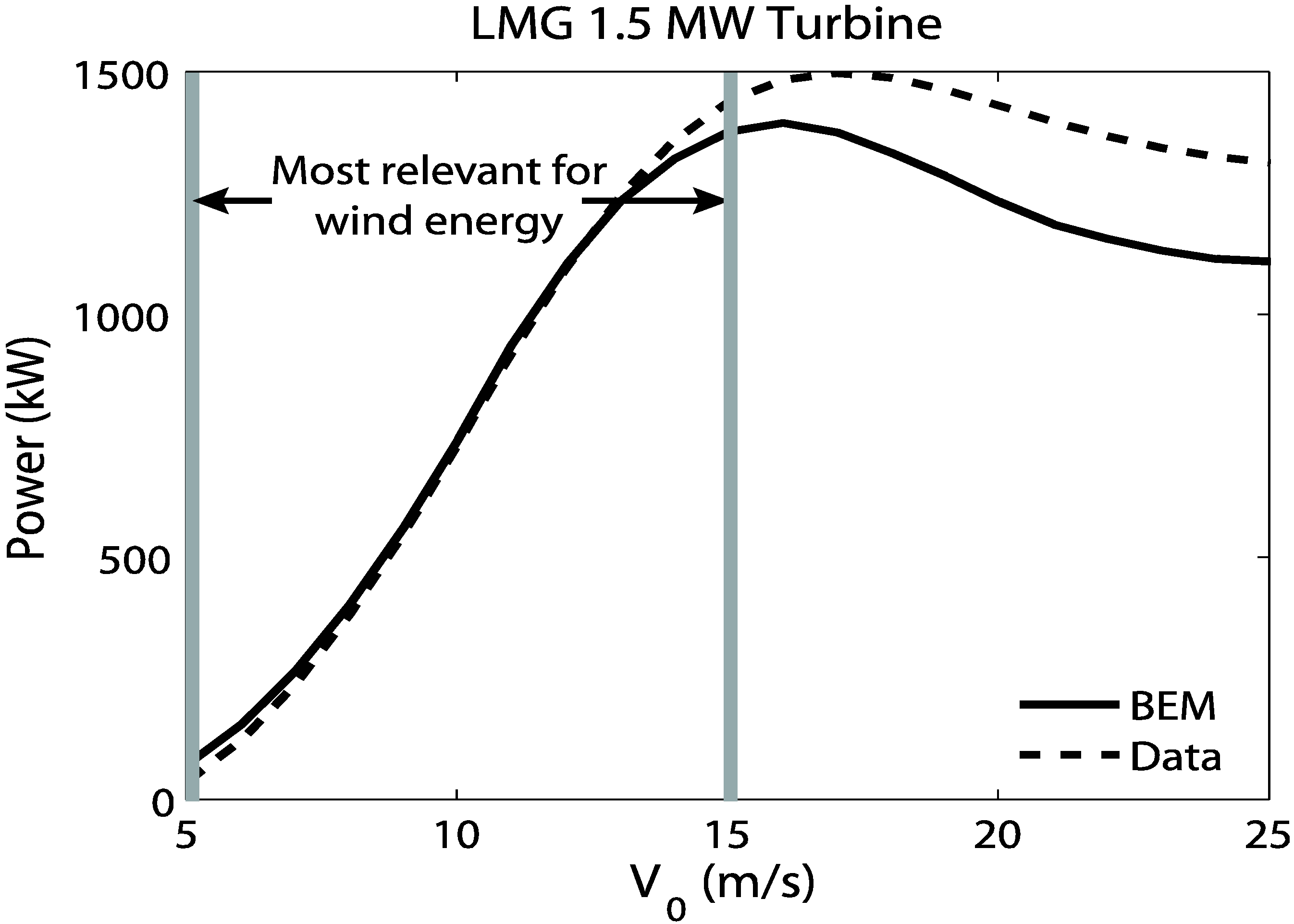
Figure 3 compares the power curves from LM Glasfiber and the BEM model. The agreement between these two power curves is much better, although in this case, the model underpredicts the power at high wind speeds. It is not clear why this occurs. The power curve was generated by the blade manufacturer so it is more difficult to determine where the discrepancy takes place.

Figure 3. LMG power comparison as a function of wind speed.

Figure 3. LMG power comparison as a function of wind speed.

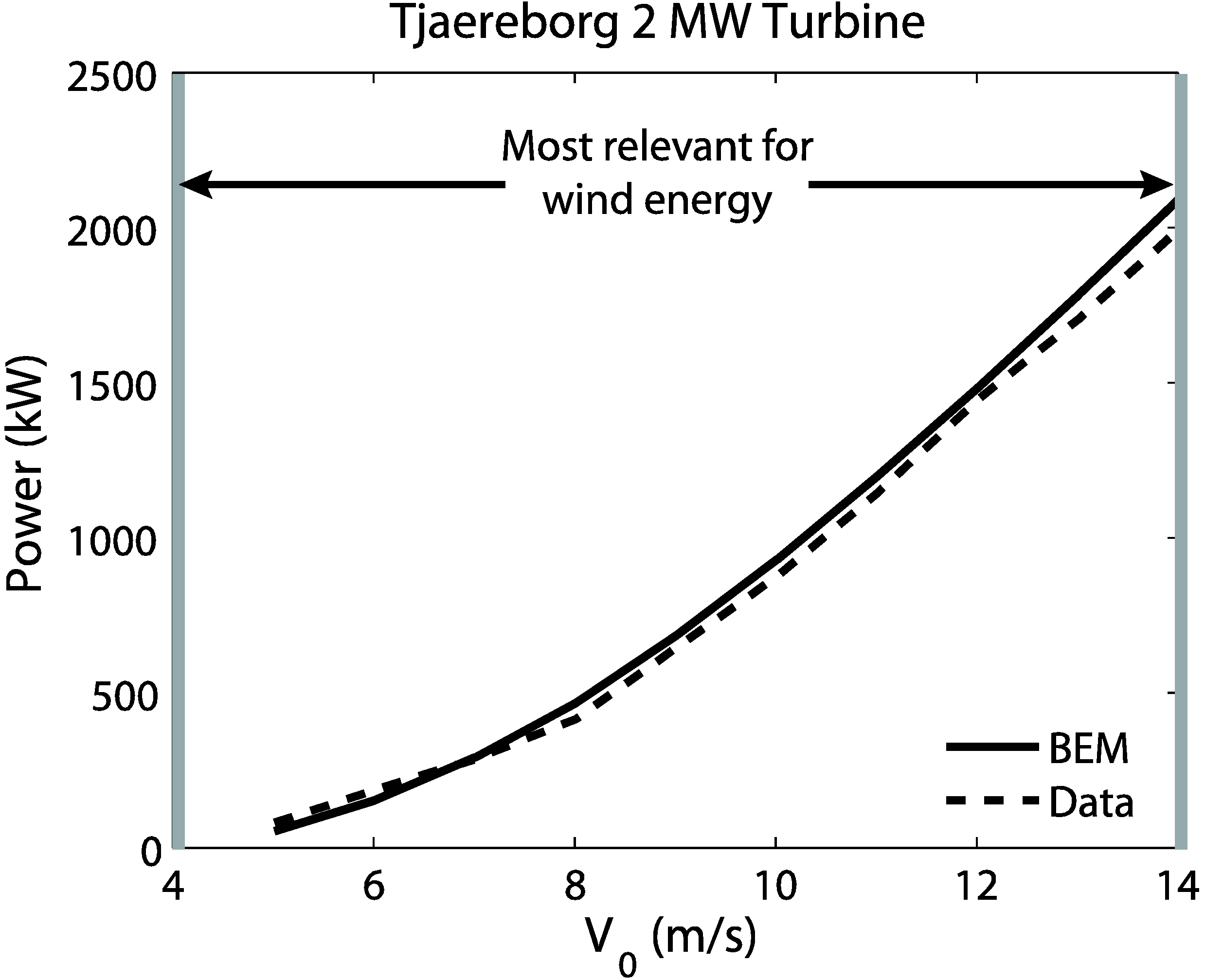
Figure 4 compares the Tjaereborg turbine and the BEM model. Here, the model performs well at low to medium wind speeds. This comparison can be done only up to the rated wind speed 14 m/s since this turbine is pitch-controlled and the pitch angle changes at higher wind speeds in order to keep power output constant. This process has not been included in the model calculations, so no comparison can be made at this time for wind speeds higher than 14 m/s.

Figure 4. Tjaereborg power comparison as a function of wind speed.

Figure 4. Tjaereborg power comparison as a function of wind speed.

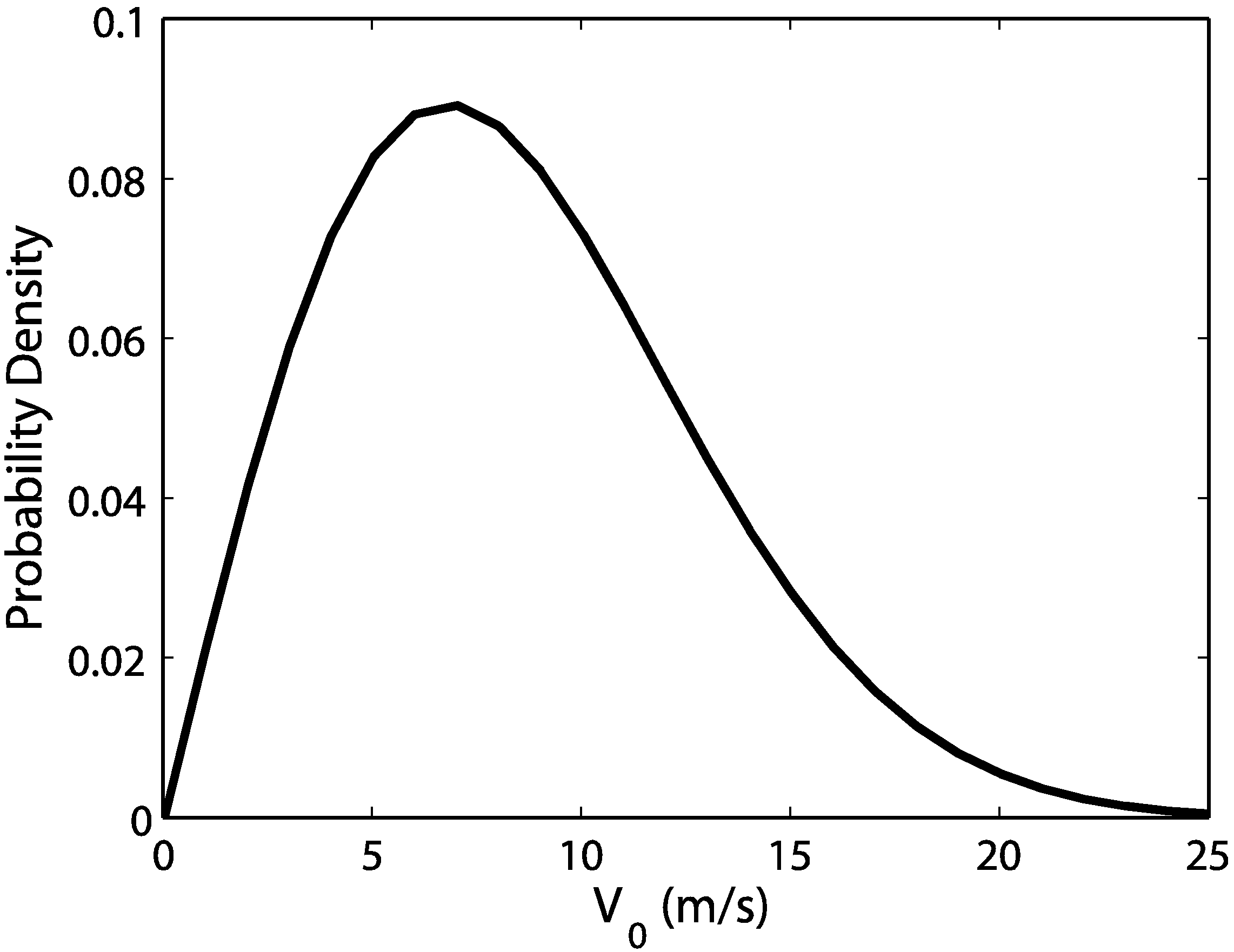
Another way of analyzing these comparisons is from the context of wind frequency distributions. From the cases shown above, the model appears to be simulating accurately the dynamics of the flow around the turbine blades up to about 15 m/s wind speed. The fact that the model does not perform well at higher wind speeds may not be important if the typical wind distribution at a wind farm site is taken into account. Although varying from site to site, the wind distribution typically follows a Rayleigh probability density function [26]:

(2)

where $b=\frac{2}{\sqrt{\pi }}\overline{V}$. The mean wind speed, $\overline{V}$, is specific to the site.

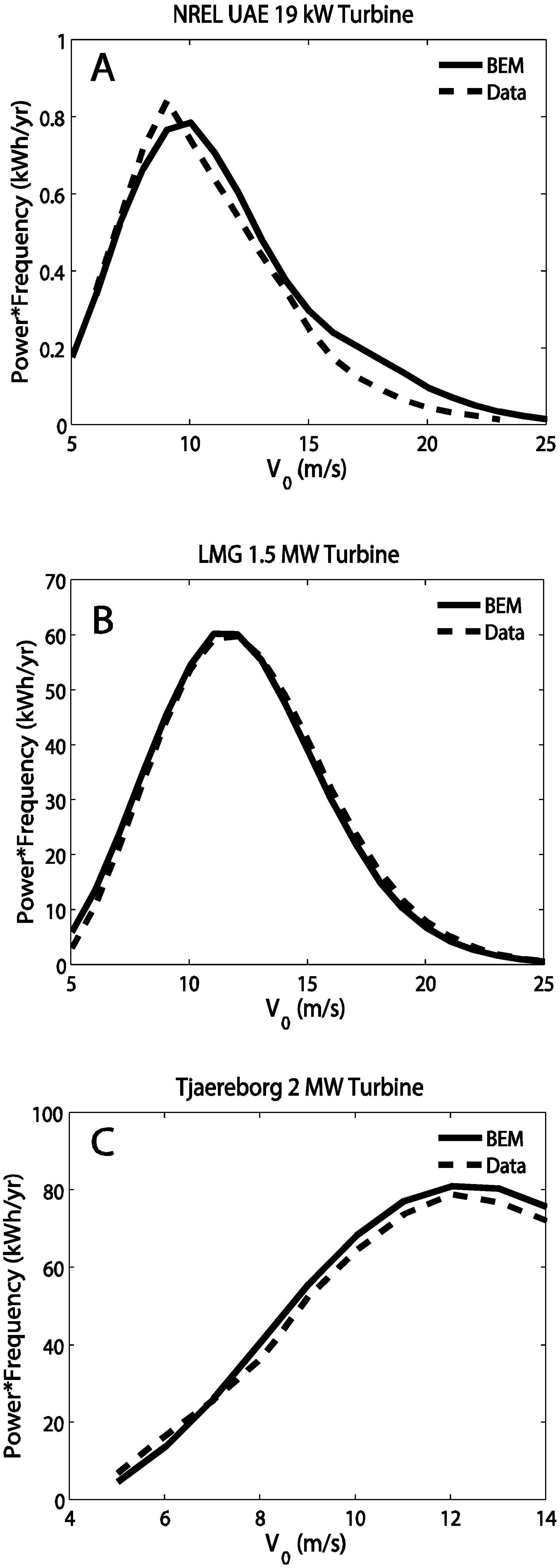
Figure 5 shows how the winds would be distributed around a specified mean wind (in this case, $\overline{V}=8.5$ m/s) with the highest probability occurring at the mean. This figure shows that there is a greater probability that winds fall within 5–15 m/s and a lower probability that they exceed 15 m/s. If the power curves are weighted by this probability distribution, the agreement greatly improves (Figure 6).

Figure 5. Rayleigh distribution function.

Figure 5. Rayleigh distribution function.

The improvement added by this wind distribution weighting is seen in the error analysis between the modeled curves and the data. To quantify the difference between the modeled power and the expected turbine power, the normalized gross error (NGE) is used. For the power curves in Figure 2, Figure 3 and Figure 4, the error is calculated as:

(3)

The resulting errors from this analysis are 38.3%, 13.1%, and 9.2%, for the NREL, LMG, and Tjaereborg cases, respectively. If the weighting by the wind frequency distribution is included, the equation for NGE becomes:

(4)

The errors then become 0.6%, 0.6%, and 0.7%, for the NREL, LMG, and Tjaereborg turbines, respectively. These results show that however imperfect, this model is sufficient for the purpose of providing more information about turbine blade-atmosphere interactions so that a better parameterization for wind farm-atmosphere interactions can be developed.

Figure 6. Previous power comparisons weighted with the Rayleigh probability distribution: (A) NREL vs. model, (B) LMG vs model, and (C) Tjaereborg vs model.

Figure 6. Previous power comparisons weighted with the Rayleigh probability distribution: (A) NREL vs. model, (B) LMG vs model, and (C) Tjaereborg vs model.

4. Energy Reduction Estimate

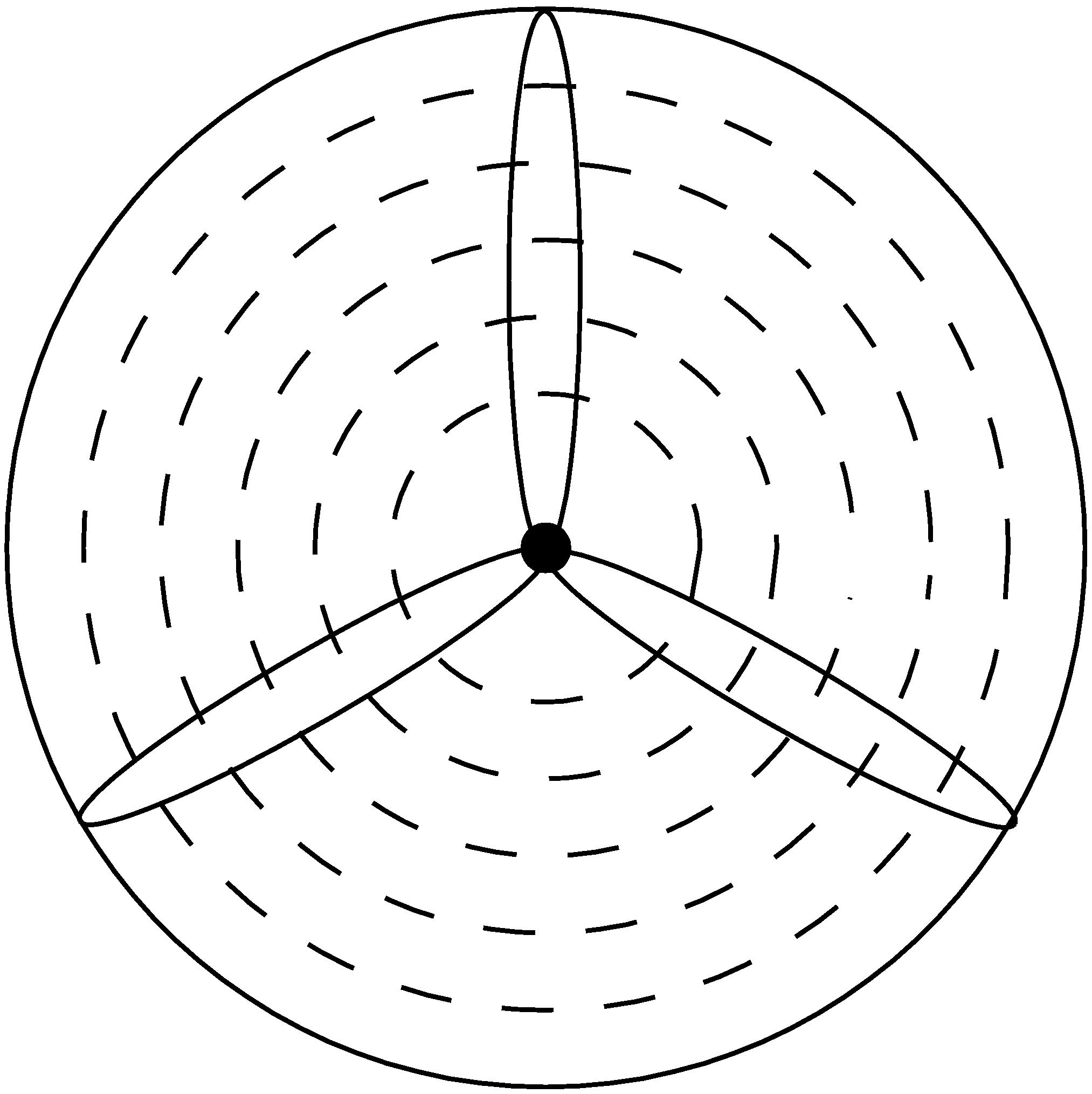
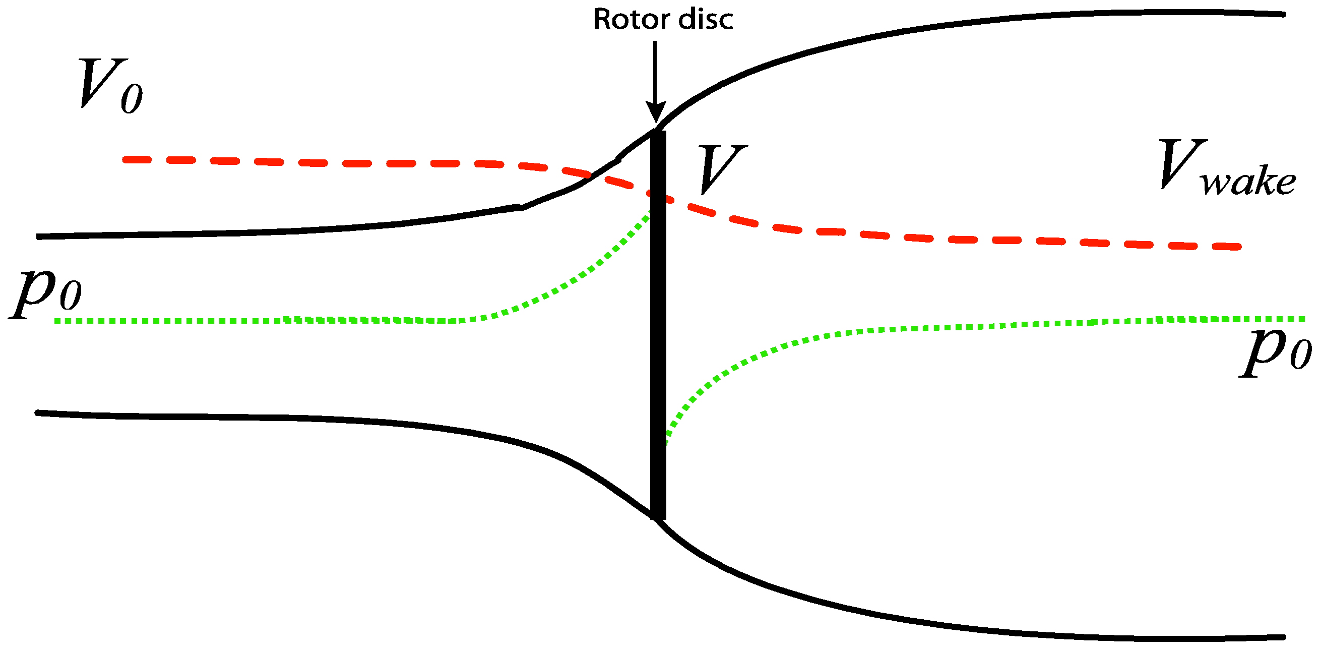
With the momentum theory from the BEM method, an analytical model can be used to estimate how much the wind is slowed down behind a rotor. From the momentum theory [13], the rotor can be approximated as an energy extracting disc, with wind speed decreasing as it approaches the rotor, and slowing even further as the energy is extracted at the rotor disc (Figure 7). The wind velocity at the disc, V, is found to be the average of the incoming velocity, V₀, and the velocity at the wake, V_wake:

(5)

Note that V_wake is not the velocity throughout the whole wake, but an estimate of the velocity in the region of the wake where the static pressure is equal to the static pressure outside the stream tube. This distance is typically 2D to 3D, where D is the diameter of the rotor [27]. The thrust, T, due to the pressure difference across the rotor can be computed as the momentum change across the disc:

(6)

The analytical model assumes that the power extracted comes from the product of the thrust force and the velocity at the disc. Using Equation (5) for V, the power becomes:

(7)

The efficiency, C_P, which is the ratio of the generated to available power in the wind, is then calculated as:

(8)

Equation (8) can be manipulated into a cubic equation for V_wake:

(9)

The efficiency is calculated by the BEM model (but can also be derived from turbine specifications), and V₀ is an input, so V_wake is easily solved for. V_wake is a measure of the axial velocity downstream of the disc and rotation in the wake is not taken into consideration. The rotation in the wake adds to the pressure drop across the disc and further reduces the kinetic energy of the flow, so V_wake calculated here is an overestimate. Including wake rotation should lead to lower axial velocities downstream (e.g., ~50% lower), but typically only near the wake edge.

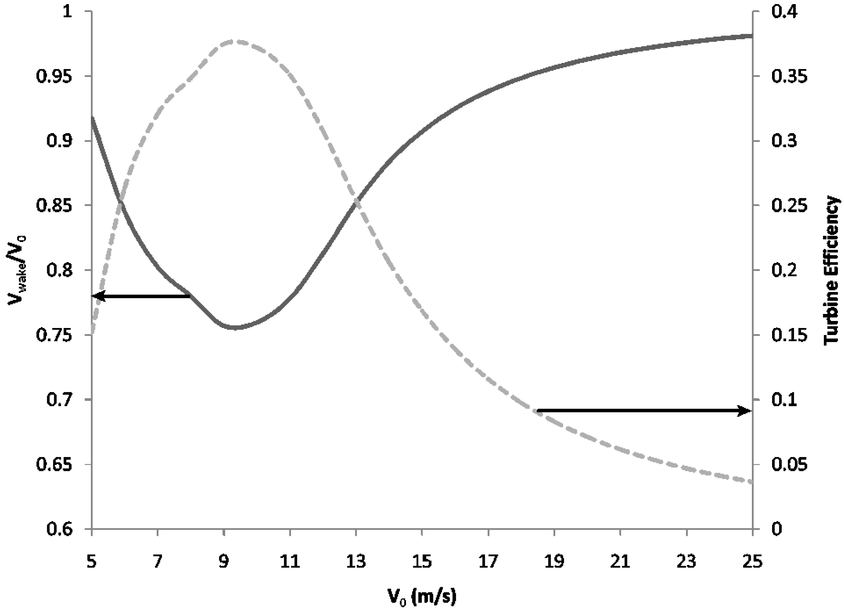
Figure 8 shows how V_wake changes with V₀ for a GE 1.5 MW turbine with a 77 m rotor diameter [28]. This turbine was chosen because it is typical of the type of turbines being erected in many wind farms today. It can be seen from the figure that the ratio of the two velocities increases with V₀ implying that less energy is taken out of the flow as the incoming wind speed increases. This makes sense as the efficiency of this specific turbine is maximum at lower wind speeds. The efficiency, C_p, is plotted together (dashed line) with the velocity to show that V_wake is small when the efficiency is high.

Figure 7. Schematic of wind speed and pressure as air flows through a wind turbine rotor.

Figure 7. Schematic of wind speed and pressure as air flows through a wind turbine rotor.

Figure 8. Change in wake velocity as a function of incoming velocity overlapped with turbine efficiency.

Figure 8. Change in wake velocity as a function of incoming velocity overlapped with turbine efficiency.

Reference 29 shows measurements of the wake velocity ratio (V_wake/V₀) to be about 50% at 2.5D downstream. Although the wind speed at which the ratio was measured was not specified, it is still possible to compare this with the minimum ratio shown in Figure 8 since this minimum is found in the 8–9 m/s wind speed range, which is the most common wind speed at many wind farms. Another measure for comparison is the relative velocity deficit, computed as:

(10)

The maximum relative velocity deficit is about 24%, occurring at 9 m/s. The average deficit is about 11%. The maximum deficit is relatively similar to maximum velocity deficits of around 32% that are observed in wind turbine wakes in the distance range of 2-3D [30]. Although different turbines were used in this observational study and measurements were taken at 32 m (lower than hub height), these maximum velocity deficit values are of the same order. Moreover, these velocity deficits are on the same order as a 20%–30% wind velocity decrease measured downwind of a large grove of pine and juniper trees, also at 32 m height [30].

In order to determine how the reduced velocity may affect energy in the atmosphere, the turbine wake velocity is used to calculate the energy loss from one turbine. Assuming the same mass of air upwind and downwind of a turbine thus cancelling the mass terms in the energy equation, the fraction of energy reduced by the turbine can be estimated as:

(11)

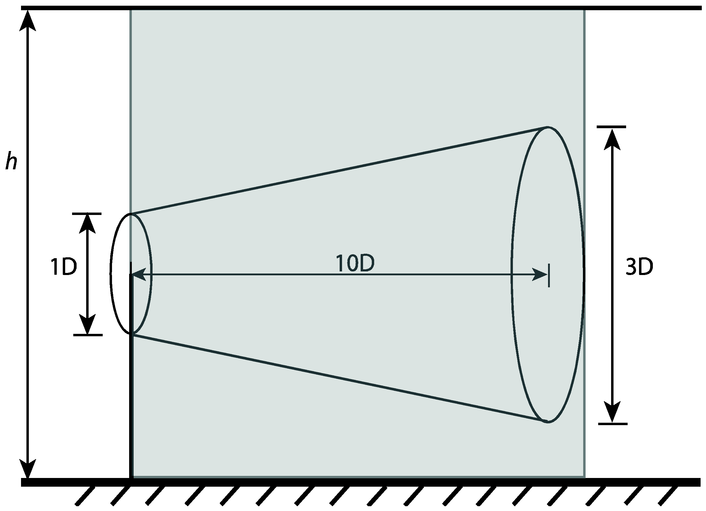
This energy is reduced only in the wake region behind the turbine however, and the rest of the air around the wake is relatively undisturbed. If it is assumed that the wake roughly follows the shape of a cone with a flat top (a frustum), then the volume of the affected air can be calculated. The volume of a frustum can be computed as:

(12)

where h_f is the height of the frustum (or, in this case, depth, since the frustum is on its side), and r₁ and r₂ are the radii of the top and base circles. Previous studies have found that the wind speed in the wake of a turbine has been recovered by more than 90% of the free stream wind speed at a distance of 10D, where D is the rotor diameter [30] and that at that distance (10D), the average wake width was about 3D. Translating these lengths into the dimensions of a frustum results in h_f = 10D, r₁ = 1D/2, and r₂ = 3D/2 (see Figure 9). The volume of the wake, S_wake, is then:

(13)

Next, a control volume can be defined that includes both the wake volume and the volume of the surrounding atmosphere. The control volume is shown in Figure 9 as the shaded region. Assuming the dimensions of this control volume are a function of the turbine spacing in a wind farm and that the turbines are spaced 3D × 10D apart (3D in the cross-wind direction, and 10D in the along wind direction) the control volume is:

(14)

where h is assumed to be 1 km (the average boundary layer height). The height of 1 km is relevant because this usually encompasses the atmospheric boundary layer, which is the layer of the atmosphere most affected by the ground and objects on it. For a single turbine, the fraction of air that is affected by the energy reduction is:

(15)

The percent of energy reduction for each turbine is then:

(16)

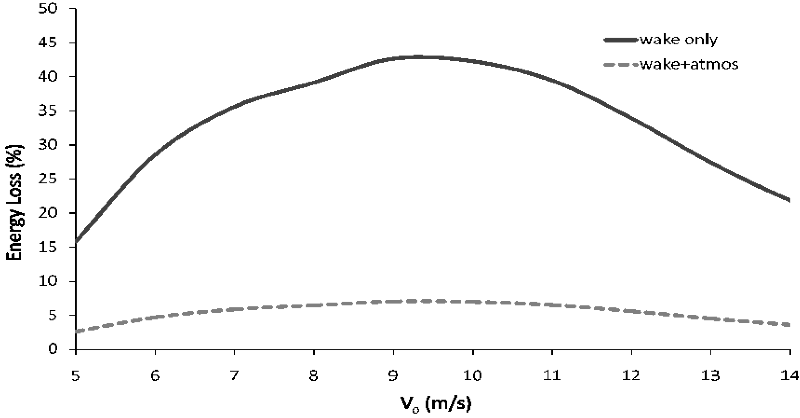
The percent of energy reduced as a function of wind speed is shown in Figure 10. The solid line shows the energy loss behind one turbine normalized by the energy of the upstream wind, as calculated by Equation (11). The dashed line shows the energy loss with the volume factored in, given that only a fraction of the air downstream of the turbine is actually affected by it (calculated using Equation (16)). The figure indicates that there can be about 40% energy loss behind a turbine. When seen in the context of the fraction of atmosphere that this loss actually applies to however, the energy reduction is not so significant.

Figure 9. Cone-like volume of air encompassed by turbine wake.

Figure 9. Cone-like volume of air encompassed by turbine wake.

Figure 10. Energy loss (%) calculated using Equation (11) (solid line) and this same loss after factoring in the fraction of atmosphere actually affected by the wake (dashed line). In the case of a wind farm with 3D × 10D spacing, this fraction is 13πD/36h (see Equation (15)).

Figure 10. Energy loss (%) calculated using Equation (11) (solid line) and this same loss after factoring in the fraction of atmosphere actually affected by the wake (dashed line). In the case of a wind farm with 3D × 10D spacing, this fraction is 13πD/36h (see Equation (15)).

It is possible to expand this analysis to determine the energy loss from many wind turbines, considering different atmospheric volumes. Two scenarios needing large installations of wind farms are examined—scenario A, which assumes that wind energy displaces the CO₂ from all fossil fuel energy sources (both electric and non-electric), and scenario B, which assumes that all onroad vehicles are replaced by wind-powered battery electric vehicles. For scenario A, two cases were analyzed. The first case assumes that wind displaces all fossil fuel energy worldwide that produces carbon. The second case assumes that wind displaces all fossil fuel carbon in the United States. Scenario B also examines two cases: replacing onroad vehicles throughout the whole U.S. and replacing onroad vehicles in California. California is of interest because it is the U.S. state with the largest vehicle density. Table 2 summarizes the cases. The energy losses from all these cases are examined both as the loss from the lower 1 km of the atmosphere (heretofore referred to as L1)—over global land and oceans—and the loss from only sections of the L1 layer that are above the land area of interest, e.g., over U.S. land.

Table 2. Different cases and scenarios used in the analysis of the energy loss from large wind farms.

Scenario	Description
A1	Replace all fossil fuel energy globally with wind
A2	Replace all fossil fuel energy in the US with wind
B1	Replace all onroad vehicles in the US with wind-powered battery electric vehicles (BEVs)
B2	Replace all onroad vehicles in California with wind-powered BEVs

Table 2. Different cases and scenarios used in the analysis of the energy loss from large wind farms.

Scenario	Description
A1	Replace all fossil fuel energy globally with wind
A2	Replace all fossil fuel energy in the US with wind
B1	Replace all onroad vehicles in the US with wind-powered battery electric vehicles (BEVs)
B2	Replace all onroad vehicles in California with wind-powered BEVs

To calculate the total energy reduction in each scenario, it is important to consider the wind speed frequency distribution. Although the Rayleigh distribution is not universal, it is general enough to make a good first approximation. Since wind farms are typically sited in regions where mean wind speeds at hub height are greater than 6 or 7 m/s, the energy loss should be applied only to locations with mean wind speeds greater than 6 m/s. The loss is then normalized by the total energy available in the wind worldwide, over the U.S., or over California. There are two values for average wind speed worldwide, $\overline{V}$, used here-over the ocean, $\overline{V}$ = 8.6 m/s, and over land, $\overline{V}$ = 4.8 m/s [31]. If the energy loss in L1 above a certain country/state is being calculated, only the average wind speed over land is used for the total available energy. Moreover, if the loss in L1 over the entire globe is calculated, both the ocean and land average wind speeds are used.

The equation used to calculate the relative energy loss for a wind farm at a site with a mean wind speed of 8 m/s, is then:

(17)

Where f₈ , f_8.6 and f_4.8 are the Rayleigh distributions centered around 8 m/s, 8.6 m/s and 4.8 m/s, respectively. The variable A_land represents the fraction of land included in the analysis. In analyzing the energy loss only over land, A_land = 1. For the analysis involving the entire ABL, A_land = 0.29, as the globe is 29% land and 71% ocean. From Equation (11), $\Delta E=V_0^2-V_3^2$ and $E_0=V_0^2$. The remaining variables are the number of turbines, N, the volume of the wake, S_wake, and the volume of the atmosphere being analyzed, S_atm. This latter volume is analogous to the control volume described earlier in the single turbine case. Here, the chosen control volume will be depend on the energy loss scenario being analyzed. It is computed as S_atm = A_sft × h where h = 1 km, and A_sfc is the surface area for each case. For example, in analyzing case A1 for L1 over the whole globe, A_sfc is the surface area of global land and oceans, but if only the loss in L1 above global land is desired, A_sfc is only the global land surface area.

The number of turbines, N, is found by dividing the energy required for each scenario, E_s, by the energy produced by a single turbine, E_t:

(18)

Since each scenario demands a different amount of energy, the number of turbines will vary from scenario to scenario. The values of the required energy per scenario are taken from Reference 32, which calculates energy consumption for the year 2007. The other energy term, E_t (kWh/yr), is calculated as:

(19)

where P_r is the turbine’s rated power (kW), CF is the turbine’s capacity factor, and γ is an efficiency factor that takes into account the energy loss due to heat, mechanical, and transmission issues. In this analysis, we assume γ = 0.85, or a loss of 15%. The capacity factor, CF, is a measure of how much energy the turbine produces over its maximum rated energy. An empirical equation for CF is:

(20)

where $\overline{V}$ is the mean wind speed at the wind farm site, P_r is the turbine’s rated power (kW), and D is its rotor diameter (m) [26]. Note that since this equation is empirical, its units do not equate.

To examine the sensitivity of the calculated energy loss, wind distributions based on different mean wind speeds, namely 7, 8, 9 and 10 m/s, were also applied to wind farm sites. Changing the mean wind speed at the wind farm sites changes the amount of energy available to be converted to electricity, thus also changing the number of turbines needed to supply the needed energy. Table 3 presents the number of turbines required for the different scenarios given the different mean wind speeds.

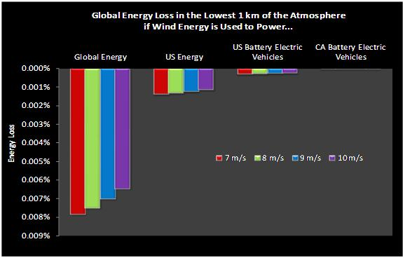
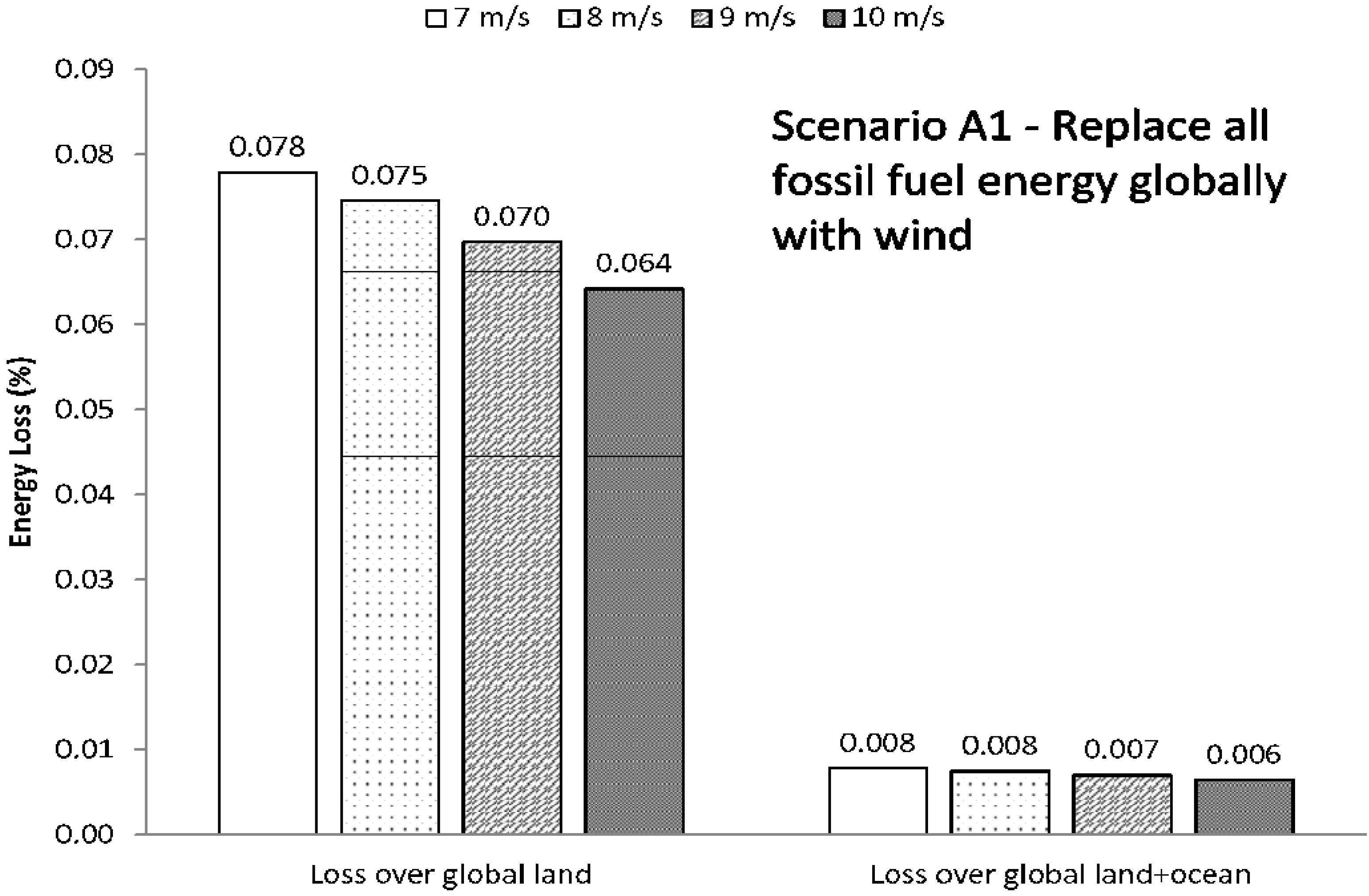
Figure 11 shows the results of this energy analysis for Scenario A1. The different bars indicate the losses given different mean wind speeds. Larger relative energy losses are found at lower mean wind speeds, where more turbines are required to generate the same energy. Relative energy losses in L1 above global land range from 0.06%–0.08%, and those above global land plus ocean range from 0.006%–0.008%. 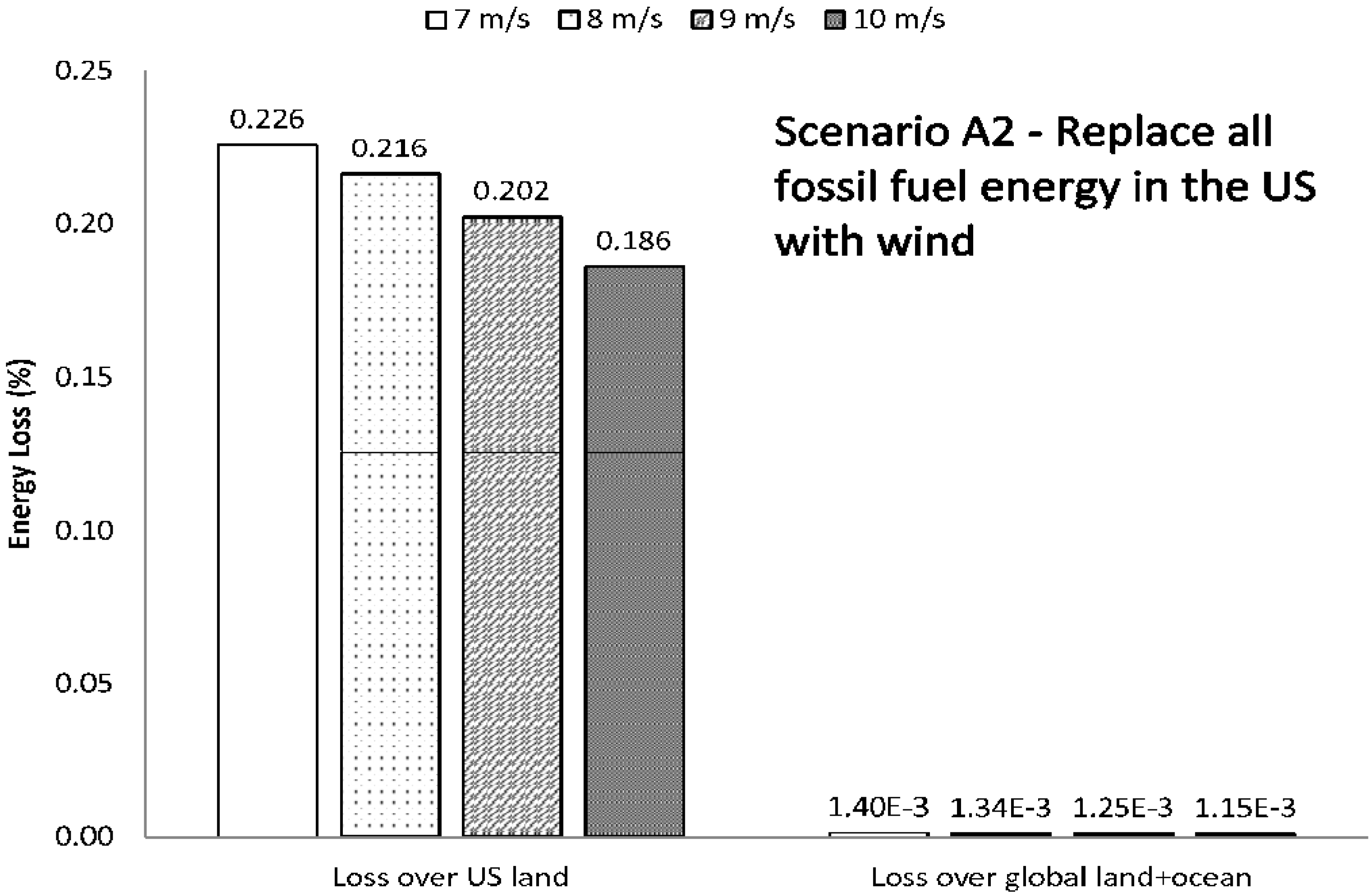The relative energy losses for Scenario A2 are shown in Figure 12. In this scenario, L1 above the U.S. loses 0.19%–0.23% of its energy, but when seen in the context of the global (land plus ocean) L1 layer, only 0.0012%–0.0014% is lost. 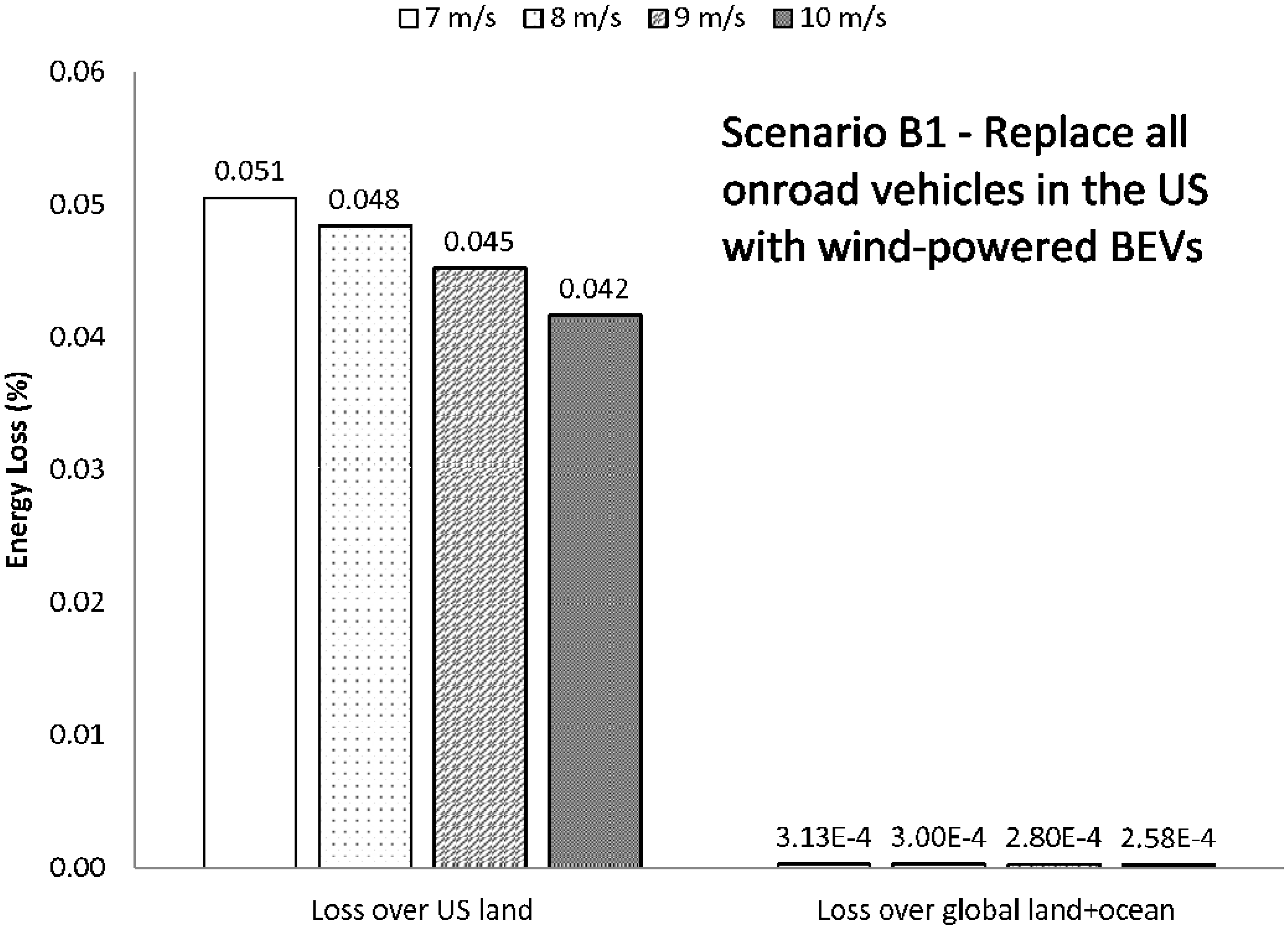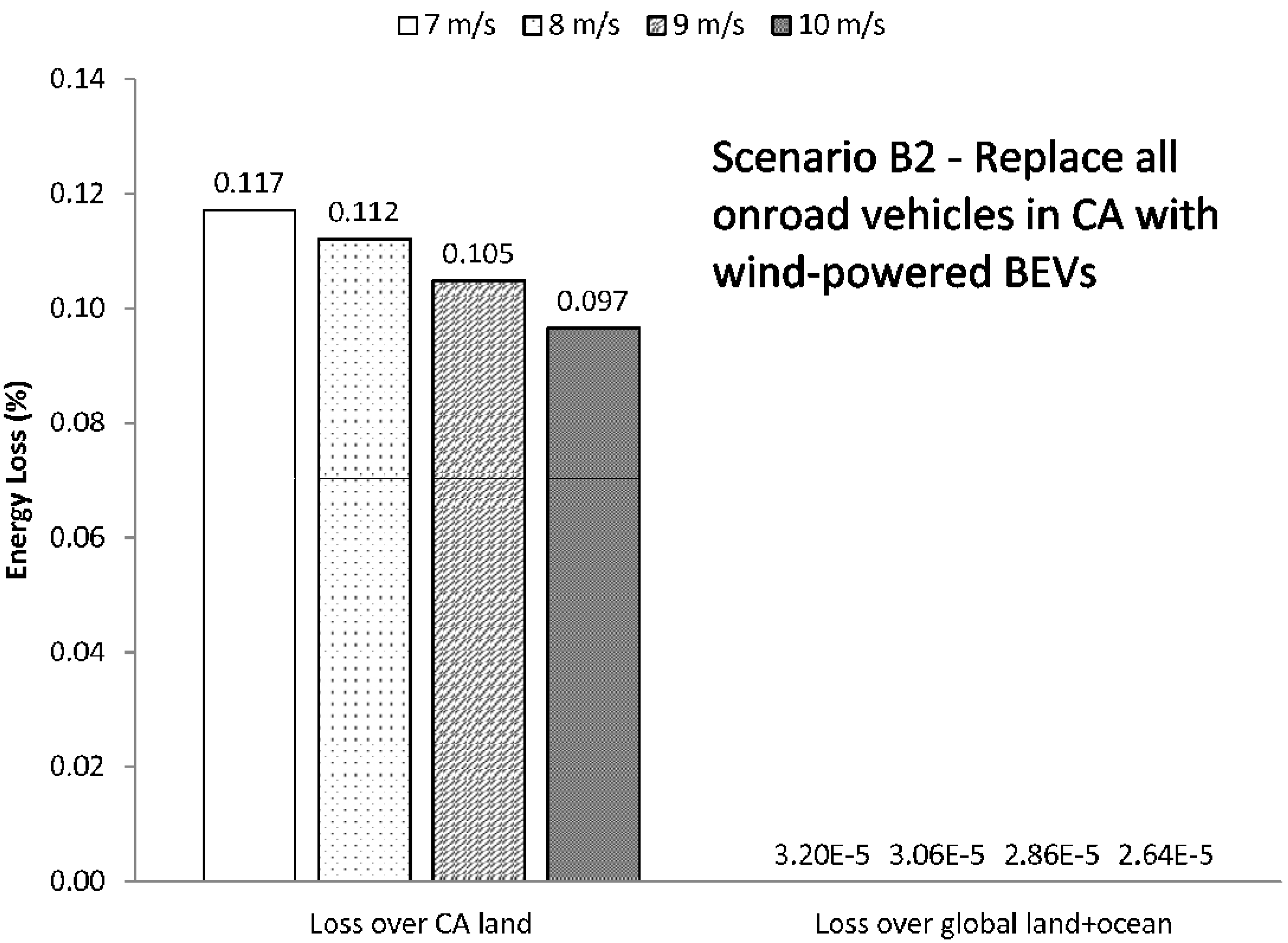Figure 13 and Figure 14 present the relative energy losses from Scenario B1 and B2, respectively. In these two cases, there is even less of an effect, even in the local L1. If all U.S. onroad vehicles were powered by wind farms, the loss in L1 over U.S. land ranges from 0.04%–0.05%. If only California vehicles, the energy loss from L1 layer over California would be 0.10%–0.12%. In L1 over global land plus ocean, a relative energy loss of 0.00026%–0.00031% results from Scenario B1, and 0.000026%–0.000032% from Scenario B2.

Table 3. Number of 1.5 MW turbines required for each scenario (see Table 2 for scenario description).

MEAN WIND SPEED (M/S)	NUMBER OF TURBINES
	Scenario A1	Scenario A2	Scenario B1	Scenario B2
7	10 million	1.8 million	400,000	40,000
8	8 million	1.4 million	320,000	33,000
9	6.7 million	1.2 million	270,000	27,000
10	5.7 million	1 million	230,000	23,000

Table 3. Number of 1.5 MW turbines required for each scenario (see Table 2 for scenario description).

MEAN WIND SPEED (M/S)	NUMBER OF TURBINES
	Scenario A1	Scenario A2	Scenario B1	Scenario B2
7	10 million	1.8 million	400,000	40,000
8	8 million	1.4 million	320,000	33,000
9	6.7 million	1.2 million	270,000	27,000
10	5.7 million	1 million	230,000	23,000

Figure 11. Energy loss (%) for Scenario A1, where wind is used to power global energy. The first set of bars indicates the relative energy loss in the entire boundary layer, while the second set indicates the losses in the boundary layer over just the global land area. The different bars represent the different mean wind speeds, 7, 8, 9, and 10 m/s, with the number of turbines needed for each mean wind speed given in Table 3.

Figure 11. Energy loss (%) for Scenario A1, where wind is used to power global energy. The first set of bars indicates the relative energy loss in the entire boundary layer, while the second set indicates the losses in the boundary layer over just the global land area. The different bars represent the different mean wind speeds, 7, 8, 9, and 10 m/s, with the number of turbines needed for each mean wind speed given in Table 3.

Figure 12. Energy loss (%) for Scenario A2, where wind farms supply U.S. energy. Similar to the previous figure, the first set of bars represents the relative loss in the entire boundary layer, and the second set represents the relative loss in the boundary layer just above the U.S. The number of turbines for each wind speed is given in Table 3.

Figure 12. Energy loss (%) for Scenario A2, where wind farms supply U.S. energy. Similar to the previous figure, the first set of bars represents the relative loss in the entire boundary layer, and the second set represents the relative loss in the boundary layer just above the U.S. The number of turbines for each wind speed is given in Table 3.

Figure 13. Energy loss (%) for Scenario B1, where all U.S. onroad vehicles are replaced with WBEV. The number of turbines for each mean wind speed case is given in Table 3.

Figure 13. Energy loss (%) for Scenario B1, where all U.S. onroad vehicles are replaced with WBEV. The number of turbines for each mean wind speed case is given in Table 3.

Figure 14. Energy loss (%) for Scenario B2, where all California onroad vehicles are replaced with WBEV. Here, the second set of bars represents the relative loss in the boundary layer just above California. The number of turbines for the different mean wind speeds are just roughly an order of magnitude less than that needed for the Scenario B1 and shown in Table 3.

Figure 14. Energy loss (%) for Scenario B2, where all California onroad vehicles are replaced with WBEV. Here, the second set of bars represents the relative loss in the boundary layer just above California. The number of turbines for the different mean wind speeds are just roughly an order of magnitude less than that needed for the Scenario B1 and shown in Table 3.

Even with higher energy consumption, the atmospheric energy loss will be minimal. Reference 33 describes a situation where all global direct electricity needs are met with wind. Moreover, other uses of fossil fuels are divided into those that can be replaced by electricity directly (such as gas heating converted into electric heating), and those that are replaced by hydrogen. The first category uses electricity powered by wind, and the second category uses hydrogen produced via electrolysis powered by wind turbines. The additional use of hydrogen increases the energy consumption, and thus the number of turbines also increases. For example, it will take three times the number of wind turbines to power a hydrogen fuel cell vehicle as it does to power an equivalent BEV. Although this study analyzes the energy consumption in the year 2030, the number of 5 MW turbines used to supply this demand can be scaled back down to 2007 values by assuming the energy demand in 2030 is 1.3 times that in 2007 [33]. This new number of 5 MW turbines for 2007 can then be scaled to the corresponding number of 1.5 MW turbines needed to supply the added hydrogen. It was found that it will take 6–21 million 1.5 MW turbines (depending on the mean wind speed) to power the world’s energy demand when hydrogen is part of the equation. This increased turbine number results in an energy loss in L1 over global land and ocean of ~0.010%–0.013%.

As indicated by these results, the energy losses from the L1 layer are very small. To put it into context, the energy reduction can be converted into a power density loss (W/m²) and compared with radiative forcing due to increased carbon dioxide (CO₂) in the atmosphere. The maximum energy loss in Scenario A1 is largest at a mean wind speed of 7 m/s. The equation used to calculate the power density loss, R (W/m²), is:

(21)

Where A_sfc = 5.1 × 10⁸ km², the surface area of the Earth. The energy loss, ∆E (J), is calculated as

(22)

where m_a is the mass (kg) of the lower 1 km of the atmosphere. In contrast to the power density loss from Equation (21), the radiative forcing due to CO₂ in the atmosphere is 1.6 W/m² [34]. A doubling of CO₂ in the absence of replacing current energy generation with wind, therefore, will have a several-order-of-magnitude larger effect on the overall climate than the atmospheric momentum loss from supplying the world’s energy demands with wind.

Furthermore, if the analysis were to be extended to include most of the atmosphere—and not just the lower 1 km—the scale height value of h = 8.7 km can be used. The scale height represents the layer of the atmosphere within which most of its mass is found. The results will be the values reported above multiplied by a factor of 0.11, which is just the ratio of the two heights, 1 km to 8.7 km. Reference 31 has found that the mean wind speed in areas that are potential wind farm sites is 8.4 m/s. The energy reduction using 8 m/s as the mean wind speed, therefore, gives the closest to realistic energy reduction scenario. Also, these energy reductions are assuming 100% penetration of wind energy, which is unlikely to happen, so even less of an effect can be expected.

5. Limitations and Context

It should be noted, however, that this analysis does not include other potential-mostly local-effects, like changes in soil moisture content, sensible and latent heat fluxes due to the increased mixing. Turbine rotors have been observed to add turbulence, or TKE, in their wakes [30,35] and Reference 11 reported changes in the vertical distribution of heat and humidity and in surface heat and moisture fluxes. Taking into consideration the increased turbulence and the changing fluxes, the modeling study in Reference 11 reports a local maximum wind speed reduction of 50% and a mean wind speed reduction of about 20% at hub height. These values can be compared to those shown in Figure 8, where the maximum velocity deficit is about 25%. Even if a 50% deficit were to be used in this analysis, because the wake volume is such a small portion of the total atmosphere, the conclusions will not be significantly changed.

The presence of turbulence can also affect power production. Relative variations in power production has been found to increase with TKE [36], especially if the TKE/RKE ratio is large. Production from upwind turbines can be influenced by turbulence generated by the environment-from uneven terrain or an unstable atmosphere, for example-while downwind turbines, if not spaced properly, can be affected by the added TKE in the wake of the upstream rotors [37]. The effect of variable power production is also not included in this analysis, but it is not believed to have a significant effect on the conclusions here. Even if the results reported here were off by a factor of 10, the conclusions would still hold.

Similarly, wind shear also affects power production. Studies done at wind energy facilities in the Midwest showed lower than expected power production during the day due to low wind shear, while there was higher than expected production during the night when the wind shear was much stronger [38]. High wind shear also adds extra load to the turbine blades, which can increase the maintenance needs and downtime of turbines. It is not clear if the addition of both turbulence and wind shear effects will have a significant difference on the range of values reported here, since it is difficult to quantify just how power production is affected by either phenomenon. In order to investigate these effects, the BEM model will have to be coupled to an atmospheric dynamics model to be able to simulate the changes in wind flow caused by both shear and high TKE.

Also not included are the effects of land use change caused by the construction and the presence of the wind farm. These can alter soil moisture content and albedo, among others, although it is most likely that these effects will be small. The turbines themselves occupy a very small footprint, and the roads are usually dirt roads with vegetation sometimes growing over them, minimizing the impact of the land use change [32]. Even with the 10 million turbines required for Scenario A1, only ~1% of global area is needed.

Even if the energy loss values reported in the previous section increased due to correcting all the limitations expressed above, the energy reduction effect due to wind farms should be taken in the context of other causes for wind speed reduction. Reference 39 simulated wind speed reductions ranging from 1%–5%, resulting in a 1.7%–8.6% wind energy loss, that correlated with increased atmospheric aerosol content over California. Losses of this magnitude can be expected over any highly urbanized area. Even if similar losses applied only to 3% of the Earth’s land area (approximately the amount of land already urbanized [40]), the energy reduction in the L1 layer due to aerosol pollution would be 0.051%–0.258%, which compares with a 0.006%–0.008% reduction due to supplying global energy with wind power. Even locally, where the energy loss from wind turbines is expected to be a maximum, other factors can also reduce wind speeds. For example, a 24% decrease in wind speed has been reported in Southeast China due to new construction and vegetation growth over a span of 20 years [41]. Any global and local atmospheric effects due to wind turbines, therefore, should be seen in the light of these other factors.

Furthermore, the energy loss from wind farms should be measured against the environmental disadvantages of maintaining fossil fuels as energy sources. Aside from mitigating global warming due to fossil-fuel combustion, using wind power can also avoid thermal pollution. Thermal power plants (TPP) have typical thermal efficiencies on the order of 30% [26]. This means that two-thirds of the energy input into the system is rejected as waste heat. A fraction of this heat is released into the atmosphere, while a majority of it is often absorbed by water, which is discharged into a nearby lake or river. The resulting increase in temperature of the water can be dangerous to the aquatic ecosystem. Assuming an average efficiency of 34%, and a typical heat production rate of 10,000 Btu/kWh [26], which translates into 10,550 kJ/kWh, the waste heat is on the order of 6,600 Btu/kWh or 6,963 kJ/kWh. Even if combined cycle gas turbines, at about 60% efficiency, or combined heat and power (CHP) systems are used, which can be up to 80% efficient, the waste heat will still be on the order of 2,000 kJ/kWh. In comparison, based on the above analysis, the maximum energy loss per year from the horizontal wind is ~2,500 kJ/kWh. Some of the loss goes into electric power production, some goes into spiraling the wake, and the rest to turbulence, which converts mechanical energy to heat. Although heat may be added to the atmosphere through this turbulent dissipation, or through the eddies transferring heat into or out of the ground, the effect and magnitude will be akin to the normal process of winds that are dissipated by surface friction. It will not be as damaging as the heat discharged by TPPs, which would otherwise not be generated if they were not in use. Thus, any heat and turbulence added to the atmosphere by turbines is significantly outweighed by the more environmentally damaging heat from the thermal power plants that these wind farms will displace.

6. Conclusions

A BEM model was developed for the purpose of determining the forces exerted onto the atmosphere by turbine blades. This provides a more detailed parameterization for the modeling of wind turbine effects on the atmosphere. The model was evaluated against three turbines, where the power curves from the turbines were compared with model-generated power curves. The best agreement between the model and data power curves occurred at wind speeds between 5–15 m/s, which is the wind speed range that is most relevant to wind energy. When the power curves were weighted with a typical wind frequency distribution—where the majority of wind speeds that occur are between 5–15 m/s—the agreement between model and data increases significantly. Based on these results, the model was found to be sufficient for the purpose of simulating the interaction between the turbine blades and the atmosphere in the context of wind power generation. Because of the resolution of this model-it uses a number of data points along a turbine blade-it will be a good tool to use to couple with an atmospheric dynamics model in order to create a better parameterization for the presence of wind farms.

The model was combined with efficiency data to estimate the energy lost from the atmosphere due to a large deployment of wind farms. The rough estimates from this model show that if the world’s energy needs were supplied by wind energy, the L1 layer over global land plus ocean would lose only 0.006%–0.008% of its energy. Even with the added energy consumption of putting hydrogen in the energy mix will only result in a loss of 0.010%–0.013%. If only the U.S. energy needs are supplied, the loss from L1 above U.S. land ranges from 0.19%–0.23%, and above global land plus ocean ranges from 0.0012%–0.0014%. Replacing U.S. onroad vehicles with wind-powered BEVs reduces energy in L1 over U.S. land by 0.04%–0.05% and over global land plus ocean by 0.00026%–0.00031%. Certainly less than 100% of the entire energy demand and vehicle energy demand will be satisfied by wind, so the actual percentages of energy loss in the L1 layer over the regions specified will likely be lower than those shown. Such losses are also estimated to be at least an order of magnitude less than energy losses due to other anthropogenic influences, such as by aerosol pollution and urbanization. Moreover, the maximum energy loss estimated in this study translates to a power density that is a few orders of magnitude less than the radiative forcing due to the doubling of CO₂ in the atmosphere. Also, any heating effects of this energy loss is outweighed by the thermal pollution that it will avert when wind farms displace the thermal power plants driven by fossil fuels.

In sum, the energy losses due to wind turbines, while high immediately downwind of a turbine, are quite small when averaged over large geographic regions, even if the entire world were powered by wind. A complete evaluation of the effects of wind turbines on local meteorology though, requires three-dimensional simulations of turbines interacting with the environment when the turbines are resolved. The BEM module discussed here can be used in such a resolved model to calculate these feedbacks.