New Approaches for Very Short-term Steady-State Analysis of An Electrical Distribution System with Wind Farms

Abstract

Distribution networks are undergoing radical changes due to the high level of penetration of dispersed generation. Dispersed generation systems require particular attention due to their incorporation of uncertain energy sources, such as wind farms, and due to the impacts that such sources have on the planning and operation of distribution networks. In particular, the foreseeable, extensive use of wind turbine generator units in the future requires that distribution system engineers properly account for their impacts on the system. Many new technical considerations must be addressed, including protection coordination, steady-state analysis, and power quality issues. This paper deals with the very short-term, steady-state analysis of a distribution system with wind farms, for which the time horizon of interest ranges from one hour to a few hours ahead. Several wind-forecasting methods are presented in order to obtain reliable input data for the steady-state analysis. Both deterministic and probabilistic methods were considered and used in performing deterministic and probabilistic load-flow analyses. Numerical applications on a 17-bus, medium-voltage, electrical distribution system with various wind farms connected at different busbars are presented and discussed.

1. Introduction

The high level of penetration of dispersed generation (DG) systems has radically changed distribution systems, and, as a result, the planning and operation of distribution networks have become critical issues.

Among the types of primary energy sources used in DG, wind generators are prevalent in medium-voltage distribution systems, and they produce a significant fraction of the energy. The wind industry has made great strides in the past 20 years, and wind turbine capacity has grown from 50 kW to 2–3 MW and more; at the same time, the unsubsidized cost of energy at the bus has decreased by more than 80%, from US$0.15–0.20/kWh a few years ago to approximately US$0.04–0.06/kWh today [1].

However, the random nature of wind makes it difficult to correctly plan and operate the distribution system. Accurate methods for forecasting wind power are essential for the economical operation of power distribution systems [2]. Moreover, a comprehensive investigation of wind power integration into an electric power system requires a careful analysis that covers time intervals that theoretically can range from a few milliseconds to several years. The impacts of wind speed variations with time on operating costs can be better understood by examining three time frames [3]:

• frequency regulation (a few seconds to about a minute);
• load following (a few minutes to a couple of hours);
• unit commitment (from several hours to one or more days into the future).

In the relevant literature, many wind-forecasting methods have been proposed with different levels of accuracy that are linked to the chosen time horizon. An extensive review is proposed in [4]. The forecasting methods can be classified as follows:

• Physical methods – methods that use physical information about the site (e.g., wind conditions at the height of turbine hubs and weather conditions). These methods are typically characterized by significant computational complexity and are mainly used for long-term forecasting.
• Statistical methods—methods that can forecast either a wind-speed/power value (“point-forecast” methods) or a wind-speed/power probability density function (“pdf-forecast” methods). Both are obtained from statistical analyses of time series from past data, and they usually employ recursive techniques. They can furnish useful information with reduced computational efforts for short-term forecasting (a few hours ahead).
• Artificial neural network methods—methods that are designed to determine the relationship between wind power and the time series from past data.
• Hybrid methods – methods that are combinations of the previous methods.

Among the various technical problems that require accurate wind forecasting, this paper addresses the very short-term, steady-state analysis of a distribution system with wind farms. Since the time horizon of interest ranges from one hour to a few hours, statistical methods are used for the wind forecast. In particular, the Persistence Method (PM), the Generalized Persistence Method (GPM), and the Nielsen Method (NM) are used as “point-forecast methods,” while the Bayesian method (BM) and the Markov method (MM) are used as “pdf-forecast methods.” When the “point-forecast” methods are used, the predicted value is used to perform a deterministic load flow for the steady-state analysis; when the “pdf-forecast” methods are used, the predicted probability density function is used to perform a probabilistic load flow calculation. It should be noted that not all authors consider the MM included in the “pdf-forecast” methods because it furnishes, strictly speaking, a time series of data in spite of a probability density function.

The first results on this subject were presented in [5]. Now, we present details on the formulation, extend both of the chosen wind forecast methods and the wind farm models, and, finally, test the models’ results on a 17-bus test distribution system. In particular, a revised Markov model for wind forecasting is proposed, and several models of wind farms are illustrated and included in the load-flow analysis, i.e., fixed-speed, semi-variable-speed, and variable-speed wind generation systems are considered.

First, the paper describes the “point-forecast methods” (Persistence Method, Generalized Persistence Method, and Nielsen Method) and the “pdf-forecast methods” (Bayesian Method and Markov Method). Then, the deterministic and probabilistic load flows are briefly discussed, focusing on the wind farm models. Finally, numerical applications and comparisons of all the methods are presented, using an actual, 17-bus, medium-voltage distribution system.

2. Very Short-Term, Steady-State Analysis of a Distribution System with Wind Farms

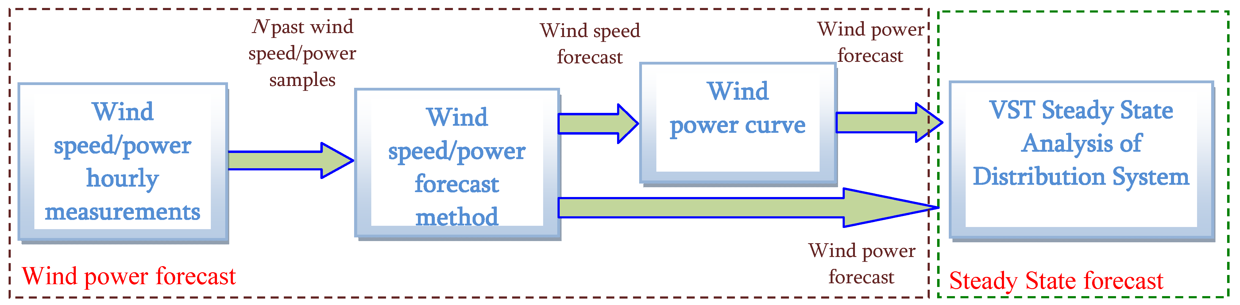
In this research, we used a two-step procedure to estimate “at hour t,” the steady-state operating condition of an electrical distribution system “at hour t + k” (k = 1, 2, ..., n). The procedure is shown in Figure 1 and consists of:

(i)

Step 1: forecast “at hour t” the wind power “at hour t + k” at the sites where the wind farms are installed; and

(ii)

Step 2: perform the very-short-term (VST), steady-state analysis of the electrical distribution system.

As shown in Figure 1, the wind power-forecast methods considered in this paper use a certain number N of hourly measurements obtained from monitoring instrumentation located where the wind turbine is installed.

Figure 1. Flow chart of the steps for a very-short-term, steady-state analysis.

Figure 1. Flow chart of the steps for a very-short-term, steady-state analysis.

These measurements, which can be wind-speed values or direct power values, are the input data for the VST wind-speed method or the power forecast method that furnishes the prediction at hour t + k with different time horizons (from one hour to a few hours), starting from knowledge of the hourly wind speed/power measurements at the sites where the wind farms are installed.

When the predictions refer to wind speed, the power production is obtained successively by using the well-known wind power curve, which determines the power output of the conversion devices as a function of wind-speed data. In the case of a wind farm composed of more than one wind turbine, the outputs of the wind turbines that are associated with the same wind farm are properly aggregated [6].

Once the power production values for the wind units are known, these values can be included among the input data for the very-short-term, steady-state analysis of the electrical distribution system using deterministic or probabilistic load flows. As previously stated, the deterministic load-flow is used when the wind “point-forecast” methods are considered, while the probabilistic load flow is used when the wind “pdf-forecast” methods are used.

In the following sections, descriptions of the wind forecast methods and the deterministic and probabilistic load flows of a distribution system with wind farms are presented in more detail.

3. Wind Power Forecast Methods

As mentioned before, several techniques have been proposed in the relevant literature for wind-speed/power forecasting. In this paper, statistical approaches are used to provide very-short-term forecasts (a few hours ahead); these methods can forecast either a wind-speed/power value (“point-forecast” methods) or a wind-speed/power probability density function (“pdf-forecast” methods). In particular, the “point-forecast” methods considered here are the Persistence Method (PM), the Generalized Persistence Method (GPM), and the Nielsen Method (NM) [7,8]. The “pdf-forecast” methods considered here were the Bayesian wind-speed prediction method (BM) proposed in [9,10] and an improved version of the Markov Method (MM) proposed in [11].

3.1. “Point-forecast” Methods [5]

All the considered “point-forecast” methods are based on the use of the hourly on-line measurements of wind power. The PM is the simplest method for making a prediction; in fact, it is based on the assumption that the wind power to predict in a future hour is highly correlated with the last observed values.

Let us assume that we want to predict the wind power ${\widehat{P}}_{t+k}$ at hour t + k; the PM provides forecasting using the following relationship:

$${\widehat{P}}_{t+k}=P_t$$

(1)

where meaning of the symbols is obvious.

The PM was developed and used by meteorologists as a comparison tool. In general, it guarantees accurate results only for very short-term time horizons (a few hours ahead).

The GPM is an extended version of the PM to a certain number of the most recent wind-power observations. It uses the average of the last N hourly-observed values of wind power to make predictions. In fact, the GPM makes forecasts using the following relationship:

$${\widehat{P}}_{t+k}=\frac{1}{N}{\displaystyle \sum _{i=0}^{N-1}{P}_{t-i}}$$

(2)

The GPM provides useful results only for cases in which the wind power is stable. Thus, the accuracy of the predictions provided by the GPM is highly dependent on the particular site and, once again, the time horizon considered.

In [8], Nielsen et al. proposed a method that combined relationships (1) and (2) in order to provide better performance than either model alone could provide. In particular, NM is based on a forecast model that is a weighting between the PM given by (1) and the mean given by (2); in fact, NM makes forecasts using the following relationship:

$${\widehat{P}}_{t+k}=c_k{P}_t+(1-c_k)\frac{1}{N}{\displaystyle \sum _{i=0}^{N-1}{P}_{t-i}}$$

(3)

where c_k is the correlation coefficient between $P_t$ and $P_{t+k}$; this coefficient is calculated using the following relationship:

$$c_k=\frac{{\displaystyle \sum _{m=k}^{N-1}\left(P_{t-m}^v{P}_{t-m+k}^v\right)}}{{\displaystyle \sum _{m=k}^{N-1}{\left(P_{t-m}^v\right)}^2}}$$

(4)

where $P_t^v=P_t-\frac{1}{N}{\displaystyle \sum _{i=0}^{N-1}{P}_{t-i}}$ From relationships (3) and (4), it is evident that, when k is small, the correlation coefficient $c_k$ is close to one, and the NM predictions are close to those made by PM; on the other hand, when k is large, $c_k$ decreases, and the forecasts made by NM are close to those made by GPM.

3.2. “Pdf-forecast” Methods

The Bayesian method (BM) and the improved Markov method (MM) are described in the following subsections.

a.

Bayesian Method

Usually, the random variable representing wind speed is modeled using the Weibull probability density function:

$$f_{\nu }(\nu |\eta \beta )=\frac{\beta }{\eta }{\left(\frac{\nu }{\eta }\right)}^{\beta -1}{e}^{-{\left(\frac{\nu }{\eta }\right)}^{\beta }}$$

(5)

where $\eta$ is the scale parameter, and $\beta$ is the shape parameter.

In [10], a Bayesian approach that uses the N hourly-observed, wind-speed samples measured until the hour t is used in a time-series model to obtain the predictive pdf $f_{v^{t+k}}$, which characterizes the random variable that represents the wind speed ν at hour t + k.

The application of the Bayesian approach is based on the definition of two random variables named “prior random variables.” To accomplish this, let us express the scale parameter $\eta$ in terms of the mean value of wind speed $\mu$ by using the following relationship:

$$\eta =\frac{\mu }{\Gamma \left(1+\frac{1}{\beta }\right)}$$

(6)

where $\Gamma (\cdot )$ is the gamma function. In order to link the mean value of wind speed at hour t (${\mu }^{\text{t}}$) to the value of wind speed at hour t - 1 ${\nu }^{t\text{-1}}$, a first-order Auto Regressive (AR) model that is based on the following relationship is used:

$$\log ({\mu }^{\text{t}})={\alpha }_1+{\alpha }_0\log ({\nu }^{\text{t-1}})$$

(7)

where α₀ and α₁ are the coefficients of the model.

The aforementioned, prior random variables required to use the Bayesian approach are obtained from relationships (5), (6), and (7); these variables are the shape parameter $\beta$ and the coefficients of the AR model, ${\alpha }_0$ and ${\alpha }_1$.

In order to obtain an approximation of the posterior distributions of parameter ${\alpha }_0$, ${\alpha }_1$, and $\beta$, a Markov Chain Monte Carlo (MCMC) approach that uses the Metropolis-Hasting (MH) algorithm was used. Once the samples from the posterior distributions of ${\alpha }_0$ and ${\alpha }_1$ are known, we can use these samples and the wind value ${\nu }^{t\text{-1}}$ to calculate the pdf of the mean value of wind speed at hour t + k. The pdf of the scale parameter distribution ${\eta }^{t+k}$ is calculated from knowledge of the ${\mu }^{t+k}$ pdf and the posterior distribution of $\beta$. Finally, using the posterior distribution of $\beta$ and the ${\eta }^{t+k}$ pdf, the predictive distribution of the wind speed ${\nu }^{t+k}$ can be obtained.

Eventually, the methodology used for “pdf forecast” furnishes a probability density function of the wind speed at hour t + k; thus, the wind power curve must be used in order to obtain the probability density function of the wind power.

It should be noted that, since the predictions are in terms of wind speed, a systematic amplification of the prediction error is added due to the relationship between wind speed and wind power.

b.

Markov Method

The Markov-based approach used in this paper is based on the assumption that the wind speed can be considered as a stochastic process (i.e., a model of a system that develops randomly in time according to probabilistic laws) with a continuous state space (linked to wind speed values) and a continuous parameter space (linked to time). This stochastic process is modeled approximately by using the discrete Markov process (Markov’s chains) [11,12,13,14]; the use of the discrete Markov process to model wind speed (and then the wind farm) was proposed in the relevant literature both for probabilistic power flow analysis and for reliability analysis of the distribution networks that have wind farms.

The approach is based on the method proposed in [11] that we have modified in order to obtain a hourly-based wind power forecast method. In particular, in [11], the authors proposed a Markov chain model that is able to generate a wind speed time series; this series is used as input to the power curve to convert wind speed to a generated power time series. In our research, the method proposed in [11] was improved by combining the time series of wind powers with the last observed wind power in order to obtain a more accurate hourly-based forecast.

The starting point of the proposed Markov-based approach is the measurements of wind speeds. Since averaging periods of one hour are generally used for wind-speed measurements, allowing variations due to turbulence and weather fronts to be separated, a time resolution of one hour also is used often. In any case, the hourly wind speed measurement data can also be divided into several time periods to determine the seasonality variations in demand.

In order to apply the Markov approach, some specific characteristics concerning the number of states, the transition probabilities, and the possible transitions among states must be assessed. In particular, the first-order Markov model proposed in [11] relies on the following assumptions.

First, the states of the wind speed must be identifiable. Then, on the basis of field measurement data, the wind speed sample record is represented by a discrete number of N wind speed states, each corresponding to an opportune range of values. The states can be fixed using wind speed intervals of constant or variable amplitude; states with variable intervals can be used in order to take into account the non-linear control characteristic of WTGUs (Wind Turbine Generation Units).

Second, the wind speed model must be stationary (i.e., the probability of making a transition from one state to another is time-invariant), and the process must lack memory (i.e., the probability of being in a given state is independent of all the past states, except for the immediately preceding state). These two requirements imply that the transition probabilities between the states are constant.

Third, the probability of a transition from a given wind speed state to another state is directly proportional to the steady state probability of the new state.

Once the number of states and the wind speed intervals for each state are defined for the Markov model, wind speed data are used to obtain an approximation of the transitional probability matrix that, as is well known, characterizes the discrete Markov process; in particular, when N states are considered, the transitional probability matrix TM is defined as:

$$\mathit{T}\mathit{M}=\left[\begin{array}{cccc}{p}_{11}& p_{12}& \cdots & p_{1N}\\ p_{21}& p_{22}& \cdots & p_{2N}\\ ⋮& ⋮& \ddots & ⋮\\ p_{N1}& p_{N2}& \cdots & p_{NN}\end{array}\right]$$

(8)

where p_ij is the probability of a transition between states i and j.

From the wind speed data, it is possible to obtain an approximation of the transitional probability matrix defined in (8); the maximum likelihood estimate for the matrix entries is:

$$p_{ij}=\frac{n_{ij}}{{\displaystyle \sum _{j=1}^N{n}_{ij}}}$$

(9)

where n_ij is the number of transitions from state i to state j encountered in the measured wind speed data.

The approximation of TM is used to generate a wind-speed time series, using the following procedure: first, the initial state i is selected. Then, a random number x between zero and unity is generated and compared to the i^th row of the matrix to find the next state; in particular, if x is lower than (or equal to) the first element in the row ($x\le p_{i1}$), the next state is state 1. If x is greater than the first element in the row and lower than (or equal to) the sum of the first two elements in the row ($p_{i1}<x\le p_{i1}+p_{i2}$), the next state is state 2. Thus, in general, if x it is greater than the sum of the first g-1 elements in the row and lower than (or equal to) the sum of the first g elements in the row (${\displaystyle \sum _{j=1}^{g-1}{p}_{ij}}<x\le {\displaystyle \sum _{j=1}^g{p}_{ij}}$), the next state is state g. The process is then repeated to find further states, using the latest state as the initial state.

Eventually, the generated wind-speed time series are used as input to the wind turbine power curve to convert wind speeds to wind power outputs.

As mentioned before, in our research, the method proposed in [11] has been improved by combining the time series of wind powers with the last observed wind power in order to obtain a more accurate, hourly-based forecast. In particular, the aforementioned generated wind power time series are modified by the following procedure:

• weight the generic element of the wind power time series with the coefficient (1-$c_k$), where $c_k$ is the correlation coefficient defined in Equation 4; and
• add the results obtained in 1. to the last observed power P_t weighted with the correlation coefficient $c_k$.

4. Load flow equations for distribution systems with wind farms

Both deterministic and probabilistic load flows are described in the following subsections.

4.1. Deterministic Load Flow

Let us refer initially to a balanced power system without wind farms, in which the busbars from 1 to n_load are load busbars and those from n_load+1 to n_bus are generator busbars. (The last busbar is the slack busbar.) In the load busbars, the active and reactive powers are assigned (PQ busbars), while in the generator busbars without the slack, active power and voltage amplitude are assigned (PV busbars). A single-phase representation of the system is adequate, and the steady state of the system is described by the following, non-linear, equation system (load-flow equations):

$$\begin{array}{l}{P}_i^{sp}=V_i{\displaystyle \sum _{j=1}^{n_{bus}}{V}_j\left[G_{ij}\cos {\theta }_{ij}\text{+}{B}_{ij}\sin {\theta }_{ij}\right],i=1,...,n_{bus}-1}\\ Q_i^{sp}=V_i{\displaystyle \sum _{j=1}^{n_{bus}}{V}_j\left[G_{ij}\sin {\theta }_{ij}-B_{ij}\cos {\theta }_{ij}\right]},i=1,...,n_{load}\end{array}$$

(10)

where: $P_i^{sp},Q_i^{sp}$ are the active powers specified at each load and generator busbar without the slack and the reactive powers specified at each load busbar, respectively; V_i, δ_I are the voltage magnitudes and arguments, respectively; $G_{ij},B_{ij}$ are the conductance and susceptance of the I - j term of the admittance matrix, respectively; n_bus, n_load are the system bus number and the load bus number, respectively; ${\theta }_{ij}$ = ${\delta }_i-{\delta }_j$.

The non-linear Equation 10 represents the active balances at load busbars and generator busbars without the slack and the reactive balance at the load busbars.

If we consider a power system with wind farms, the equations that describe the models of the WTGUs must be integrated in the previous load-flow equations. These models depend on the whole wind energy conversion system and can be classified on the basis of the presence or absence of power electronic devices or with reference to speed characteristics. In this paper, we used the classification based on speed, so the models can be classified as follows [15]:

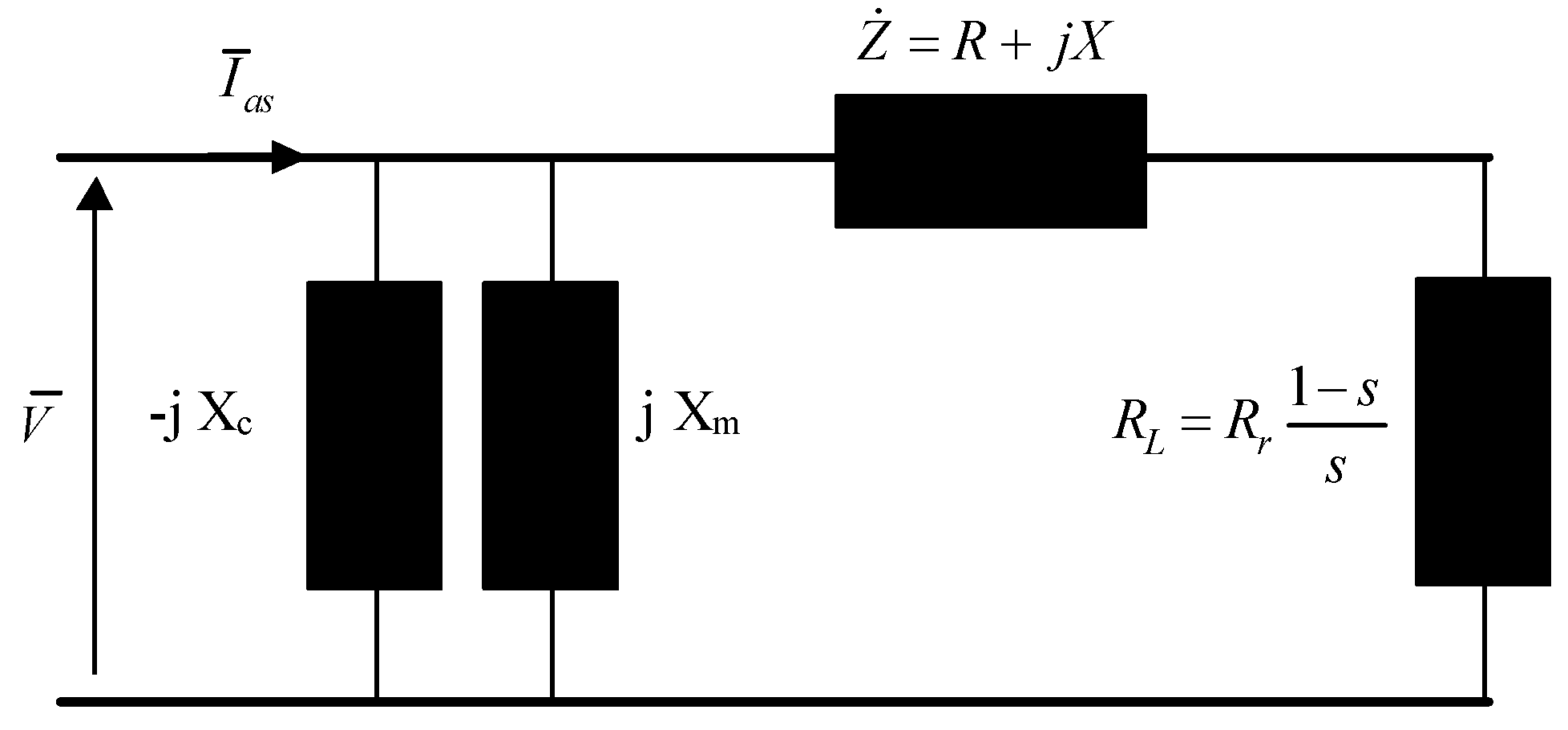
• fixed speed WTGUs (induction generators directly connected to the distribution system that are driven by wind turbines with either a fixed turbine blade angle or a pitch controller to regulate the blade angle);
• semi-variable-speed WTGUs (induction generators with a rotor-resistance converter); and
• variable-speed WTGUs (doubly-fed induction generators or synchronous/induction generators with full-scale static converters).

For each of the above categories, several models have been proposed in the literature, some of which are presented in the following and used in the numerical application.

a.

Fixed-speed WTGUs

Fixed-speed WTGUs are induction generators directly connected to the distribution system. Since the variations of the rotor speed of an asynchronous generator are very small, such generators are considered as fixed-speed WTGUs.

Two main different categories of fixed-speed WTGU models exist, i.e., the PQ-bus model and the RX-bus model, and they are considered here to be included in the load flow analysis [6].

In the PQ-bus model, WTGUs are described by their active and reactive powers; in the RX-bus model, WTGUs are described by an equivalent impedance once the parameters and the slip of the generator are known.

Both the PQ-bus model and the RX-bus model were proposed starting from the well-known equivalent circuit of an asynchronous generator in a steady-state condition (Figure 2) or similar. In Figure 2, $\overline{V}$. the bus voltage, X is the sum of the rotor X_r and stator X_s leakage reactances, X_m is the magnetizing reactance, X_c is the reactance of the capacitor bank used for power factor improvement, R is the sum of the stator R_s and rotor R_r resistances, and s is the slip.

Figure 2. Equivalent circuits of an asynchronous generator.

Figure 2. Equivalent circuits of an asynchronous generator.

In the PQ-bus model, the generated active power P is assumed to be equal to the wind turbine mechanical power output P_m (wind power forecast, Step 1, Subsection 2.1), if active power losses are neglected.

The reactive power Q is calculated using a quadratic equation that depends on the active power. In particular, the following expressions are proposed (Figure 2):

$$Q=-\left(V^2\frac{X_c-X_m}{X_c{X}_m}+X\frac{V^2-2R{P}_m}{2\left(R^2+X^2\right)}-X\frac{\sqrt{{\left(V^2-2R{P}_m\right)}^2-4P_m^2\left(R^2+X^2\right)}}{2\left(R^2+X^2\right)}\right)$$

(11)

$$Q=-\left(V^2\frac{X_c-X_m}{X_c{X}_m}+\frac{X}{V^2}{P}_m^2\right)$$

(12)

The dependence of reactive power on active power and voltage are clearly evident in the two preceding equations.

In [6], Equation 12 was used, and the model was included in a Newton-type algorithm. All busbars with WTGUs are considered to be classical PQ busbars, but, in contrast to a conventional PQ-bus, in which reactive power is assigned off-line and remains constant during iterations, the reactive power is considered to vary across iterations, and its value is updated during each iteration on the basis of the value of the current bus voltage.

In the RX-bus model, as previously mentioned, the WTGU is represented by an impedance that is based on the steady-state model of the asynchronous generator.

Two sequential, iterative processes are used to obtain the state of the system: (1) the classical load-flow analysis in which the WTGU bus is considered a PQ-bus with active and reactive powers equal to zero with the machine admittance, ${\dot{Y}}_g=1/{\dot{Z}}_g$, included in the system admittance matrix and (2) the calculation of the slip of the machine (needed to calculate the machine admittance) using the balance between the mechanical power of the wind turbine and the electrical machine. A unified solution method that simply solves all equations together (load-flow equations and the equation that equates the mechanical power of the machine and the power taken from the wind) also can be performed.

b.

Semi-variable speed WTGUs

Semi-variable speed WTGUs are basically WTGUs with pitch-controlled wind turbines and induction generators with wound rotors connected to an external resistance, which is varied by means of a power electronic converter. Once again, the WTGU bus can be considered a PQ-bus in the load-flow equations.

The active power P is assumed to be equal to the wind turbine mechanical power output P_m of the WTGU. With reference to the reactive power, it should be noted that the rotor resistance is variable and unknown, as is the machine slip; to take these facts into account, in [15], a very simple procedure is suggested that reduces the two unknowns (slip and rotor resistance) to only one unknown by considering that the expressions of active and reactive power outputs can be written as a function of only one unknown R_eq = R_r /s, obtaining:

$$\begin{array}{l}{R}_{eq}=\min \left|\frac{-b_1\pm \sqrt{b_1^2-4a_1{c}_1}}{2a_1}\right|\\ \text{where}\\ a_1=P\left[R_s^2+{\left(X_m+X_s\right)}^2\right]-V^2{R}_s^2\\ b_1=2P{R}_s{X}_m^2-V^2{X}_m^2\\ c_1=P{R}_s^2{\left(X_m+X_s\right)}^2+P{\left(X_m^2-\left(X_m+X_r\right)\left(X_m+X_s\right)\right)}^2-V^2{R}_s{\left(X_m+X_r\right)}^2\end{array}$$

(13)

Once R_eq is known, the reactive power output can be calculated with the following equation:

$$Q=-\frac{\left\{R_{eq}^2\left(X_m+X_s\right)-\left[X_m^2-\left(X_m+X_r\right)\left(X_m+X_s\right)\right]\left(X_m+X_r\right)\right\}{V}^2}{{\left\{R_{eq}{R}_s+\left[X_m^2-\left(X_m+X_r\right)\left(X_m+X_s\right)\right]\right\}}^2+{\left[R_{eq}\left(X_m+X_s\right)+R_s\left(X_m+X_r\right)\right]}^2}$$

(14)

The above-mentioned PQ-bus model can be included also in a sweep-based algorithm, converting the powers in complex current injections as well.

c.

Variable-speed WTGUs

Variable-speed WTGUs are WTGUs with pitch-controlled wind turbines that have either doubly-fed induction generators (DFIG) or asynchronous and synchronous generators with back-to-back converters (GBBC).

Doubly-fed induction generators are asynchronous machines that are directly connected to the grid with a wound rotor and slip rings; a converter is connected to the rotor circuit through the slip rings that control the speed with a variation of ± 30% around the synchronous speed and control both active and reactive output power. Generators with back-to-back converters are connected to the grid through a full-power, voltage-source converter so that active and reactive output power can be controlled.

The WTGU controllers usually operate so that the active power output is equal to the maximum power at wind speeds below the rated speed and equal to rated power above rated wind speed.

Since the reactive power can be controlled by converters, it can be assumed that they are assigned on the basis of the set point; in some cases, the controllers operate so that the power factor is maintained at a fixed value.

Then, both WTGUs were modeled as an equivalent PQ-bus.

Eventually, P was assumed to be equal to the wind turbine mechanical power output P_m of the WTGU. For the reactive power output, the following expression applies:

$$\begin{array}{l}Q=-Q^{sp}\\ \text{or}\\ Q=-P\frac{\sqrt{1-{\cos }^2{\left(\mathsf{\phi }\right)}^{sp}}}{\cos {\left(\mathsf{\phi }\right)}^{sp}}\end{array}$$

(15)

where Q^sp and $\cos {\left(\mathsf{\phi }\right)}^{sp}$ are the specified values of reactive power and power factor, respectively.

Once again, either the well-known Newton-Raphson algorithm can be applied to solve the load-flow equations, including the WTGU models or the above-mentioned PQ-bus model can be included in a sweep-based algorithm, converting the powers in complex current injections as well.

4.2. Probabilistic Load Flow

As previously shown, when the wind forecast is a probability density function, a probabilistic load flow must be performed for VST steady-state analysis. Several probabilistic load-flow techniques can be applied for this purpose (e.g., Monte Carlo simulation, convolution process, and special distribution functions), as shown in [16]. In this paper, all of the load-flow equations of a distribution system with wind farms shown in the previous subsection are included in a Monte Carlo simulation procedure in order to obtain the pdfs of the output variables.

Please recall that the Monte Carlo procedure consists of solving the load-flow equations (including the wind farm models) several times, with each iteration using as input data one set of the input random variables (loads and wind power productions) generated according to their assigned probability density functions (pdfs). The process is repeated a sufficient number of times to obtain adequate accuracy in the estimation of the output, random, variable pdfs.

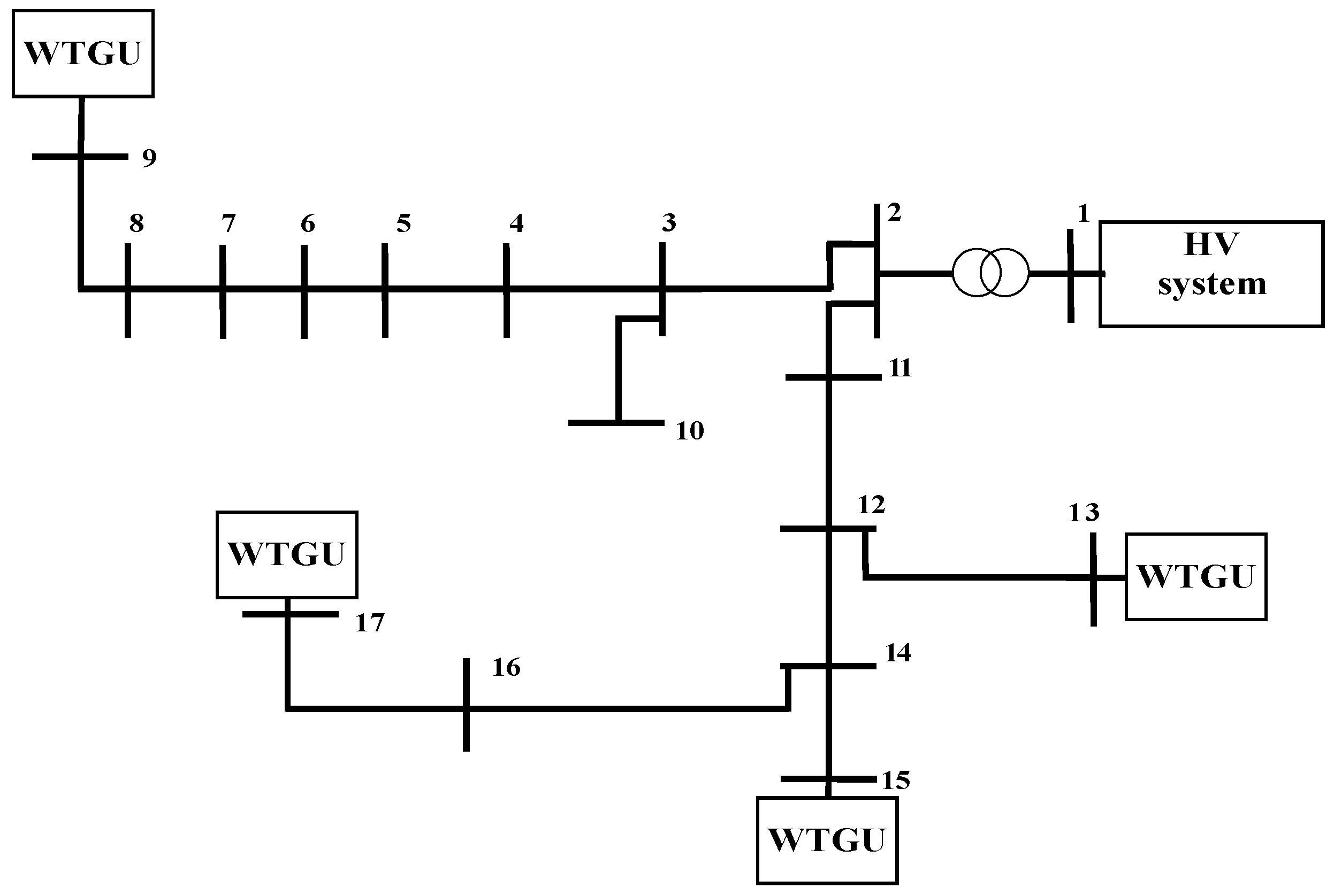
5. Experimental Section

A comparison of the proposed VST steady-state analysis was conducted with reference to a medium-voltage distribution system (Figure 3); this system contains 16 busbars at 12.5 kV and one busbar (#1) at 138 kV. The main data of the considered test system can be found in [17]; the system base is 10 MVA.

In the distribution system shown in Figure 3, four wind turbine generation units are installed, and the four units are as follows:

-

1.0 MW, semi-variable-speed WTGU at bus #9;

-

1.0 MW GBBC, variable-speed WTGU at bus #13;

-

1.0 MW DFIG, variable-speed WTGU at bus #15;

-

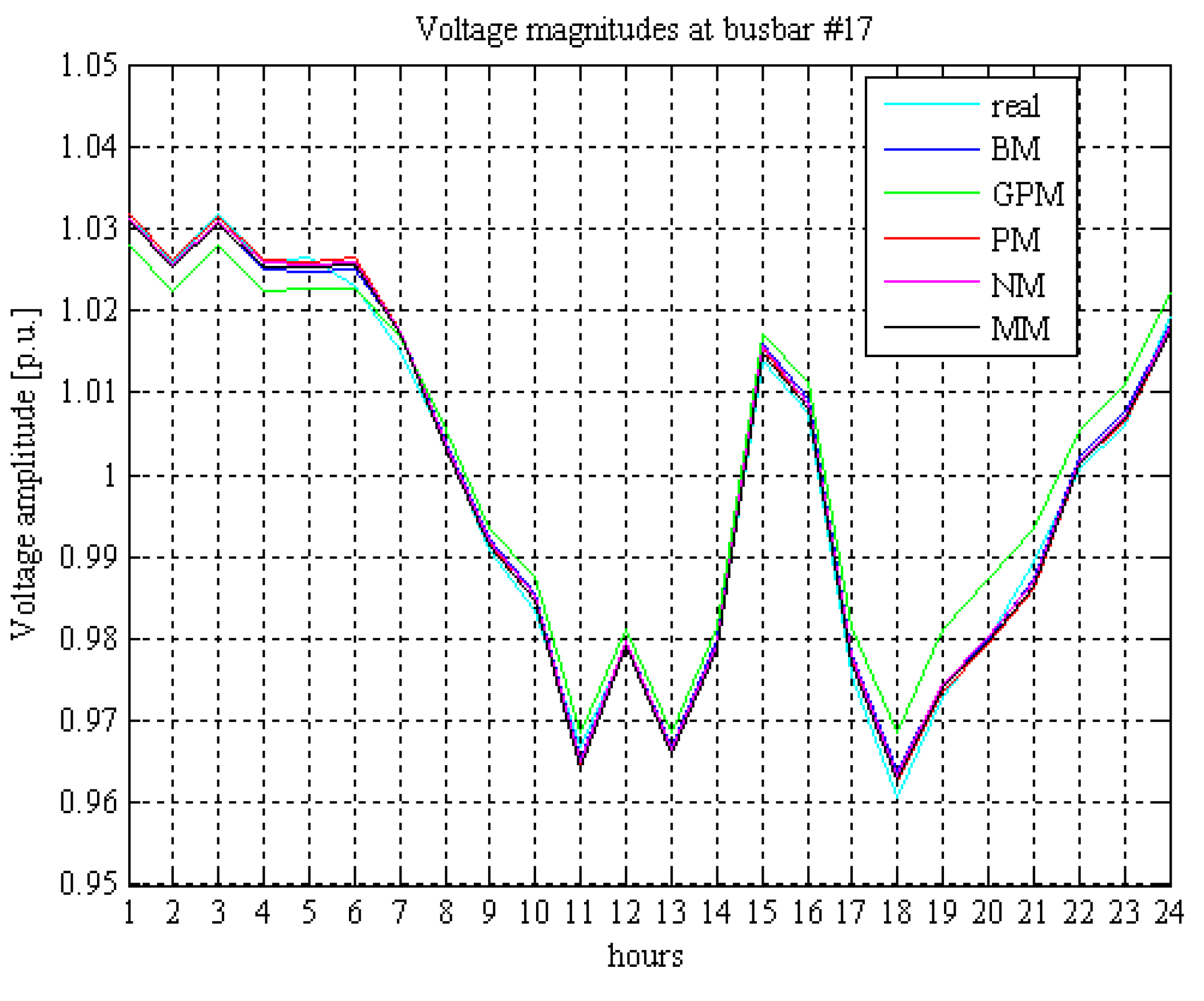
1.0 MW stall-regulated, fixed-speed WTGU at bus #17.

The daily load variations shown in Figure 4 were considered at each node. The load variations are expressed in p.u. of the rated load powers that can be found in [17]. In the probabilistic load-flow applications, the hourly loads have been considered to be characterized by Gaussian pdfs, the mean values of which are the rated powers (taking into account the daily load variations shown in Figure 4); the standard deviations are assumed to be 10% of the mean values.

The hourly steady-state analyses of the distribution system were conducted with reference to a summer day. To consider a real case, wind-speed samples were obtained from the Royal Netherlands Meteorological Institute (http://www.knmi.nl/samenw/hydra/index.html). These data refer to the measured data at wind stations Texelhors and De Kooy.

The predicted hourly power generated by wind units was obtained by using the point-forecast and pdf-forecast methods described in Section 3 (with k = 1) and by using the observed wind-speed samples of six days before (N = 144 hours). In order to compare all methods with the same input data (for the forecasting methods that require wind power as input data), the wind speed measurements were converted to wind power using the proper wind power curve.

In particular, PM, GPM, and NM were used for the N wind-power samples that were obtained by applying the WTGU models to the N wind-speed samples.

With reference to the MM method, the time series of the hourly wind power were obtained by applying the procedure shown in Section 3.2.b. First, N wind-power samples were obtained by applying the WTGU models to the observed N wind-speed samples; then the N wind-power samples were used to obtain the predicted power at hour t+1.

Figure 3. 17-busbar, balanced, three-phase test distribution system [17].

Figure 3. 17-busbar, balanced, three-phase test distribution system [17].

Figure 4. Variation of daily loads.

Figure 4. Variation of daily loads.

With reference to the BM method, the pdfs of the hourly wind speed were obtained by applying the procedure shown in Section 3.2.a First, the prediction of the wind-speed pdf of the t + 1 hour was obtained using the observed N wind-speed samples; then, the wind-power pdf was obtained by applying the WTGU models to the samples of the predicted wind-speed pdf.

In order to show examples of the intermediate results, Figure 5 compares the hourly forecasted mean value of the wind speed obtained with the BM method with the actual wind-speed value at busbar #17 (also the spread between minimum and maximum values of the pdf is shown in Figure 5); good predictive behavior is clearly evident. (The same happens for the wind station at the other busbars.)

Figure 5. BM-predicted values (minimum, mean, and maximum values) and measured values of the hourly wind speed at the site where the WTGU is connected to busbar #17.

Figure 5. BM-predicted values (minimum, mean, and maximum values) and measured values of the hourly wind speed at the site where the WTGU is connected to busbar #17.

In addition, Figure 6 compares the BM and MM mean values of the hourly forecasted wind power with the actual wind power values at busbars #13 and #17. Also, in Figure 6, the hourly forecasted wind power values obtained by applying the other methods are shown.

The results of Figure 6 show that, as expected, PM furnishes a simple shifted curve of actual powers. Moreover, the GPM, NM, MM, and BM predictions generally have values lower than the ones obtained by PM. In particular, GPM predictions, as expected, were slightly variable during the 24-hour period due to the significant influence of the mean value of the last N measured powers in the application of relationship (2).

Figure 7 and Figure 8 show the voltage profile of the network busbars obtained by means of the chosen forecasting methods at four different hours, characterized by low, high, and medium load levels, respectively. The voltage profile in case of BM and of MM refers to the voltage mean values.

All methods, except GPM, perform very well; only the results obtained with the GPM method were not strictly close to the real results. This was mainly due to the fact that the last N power samples used in relationship (2) for the GPM prediction of the power generated by the WTGUs were greater than the actual power values.

As a further example of the results obtained, Figure 9 shows the values (expressed in p.u.) of the voltage magnitudes over a 24-hour period at busbar #17. Once again, the voltages in cases of BM and MM refer to the voltage mean values.

As a further example of important electrical quantities to be taken into account in a distribution system with wind farms, in Figure 10, the hourly power losses (expressed in kW) during 24 hours are shown, while, in Figure 11, the cumulated daily values of power losses are reported. In the cases of BM and MM, the mean values of predicted powers are considered.

All of the methods, except GPM, furnish very good results for the pre-selected time horizon. It should be noted that, for all of the methods, the voltage errors were significantly lower than the errors in the WTGU values. Clearly, this is due to the fact that the WTGU power values are only a fraction of the power required by the distribution system’s loads, so that the prediction errors in the wind power values have a reduced effect on the voltage value predictions.

Figure 6. BM and MM mean values; GPM, PM, NM predicted values; and measured values of the hourly WTGU power at busbar #13 (a) and at busbar #17 (b).

Figure 6. BM and MM mean values; GPM, PM, NM predicted values; and measured values of the hourly WTGU power at busbar #13 (a) and at busbar #17 (b).

Figure 7. Voltage profile of the network at hour 1 (a) and at hour 11 (b).

Figure 7. Voltage profile of the network at hour 1 (a) and at hour 11 (b).

Figure 8. Voltage profile of the network at hour 19 (a) and at hour 20 (b).

Figure 8. Voltage profile of the network at hour 19 (a) and at hour 20 (b).

Figure 9. Voltage amplitudes over a 24-hour period at busbar #17.

Figure 9. Voltage amplitudes over a 24-hour period at busbar #17.

Figure 10. Power losses during a 24-hour period (BM and MM mean values).

Figure 10. Power losses during a 24-hour period (BM and MM mean values).

Figure 11. Daily power losses (BM and MM mean values).

Figure 11. Daily power losses (BM and MM mean values).

Figure 12. Voltage amplitudes during 24 hours at busbar #17 in the absence of wind generators.

Figure 12. Voltage amplitudes during 24 hours at busbar #17 in the absence of wind generators.

Figure 13. Power losses during 24 hours in the absence of wind generators.

Figure 13. Power losses during 24 hours in the absence of wind generators.

Finally, in order to clearly show the significant influence of the wind farm on the operation of the distribution system, Figure 12 and Figure 13 show the voltage profiles and the power losses in absence of the wind farm.

By comparing the voltage amplitudes shown in Figure 12 with the ones of Figure 9, it is evident that the greater increase of voltage arises during the night; if we compare the hourly power losses of Figure 13 with the ones reported in Figure 10, we observe that, as expected, in the presence of the wind generation there is a significant reduction of losses, especially when the amount of wind generation with respect to load level is higher.

4. Conclusions

A very short-term, steady-state analysis of an electrical distribution system with wind farms was conducted. The analyses were based on appropriate wind forecasting methods and the solutions for non-linear load flow equations. Both deterministic and probabilistic methods were used, and several wind farm models were evaluated, i.e., fixed-speed, semi-variable-speed, and variable-speed wind generation systems.

Numerical applications of a test distribution system were discussed, considering the various wind farm models.

The main outcomes of the analyses were:

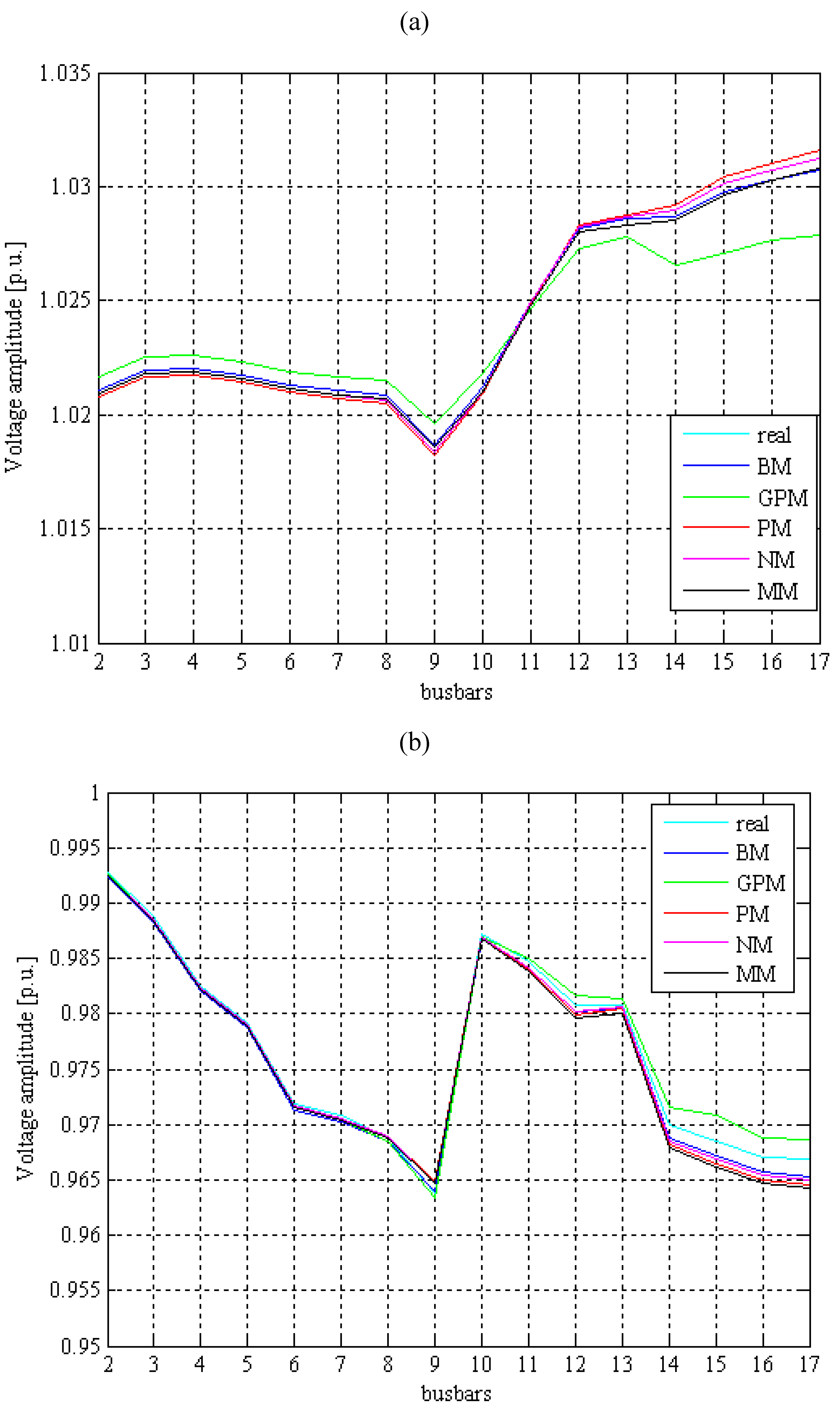
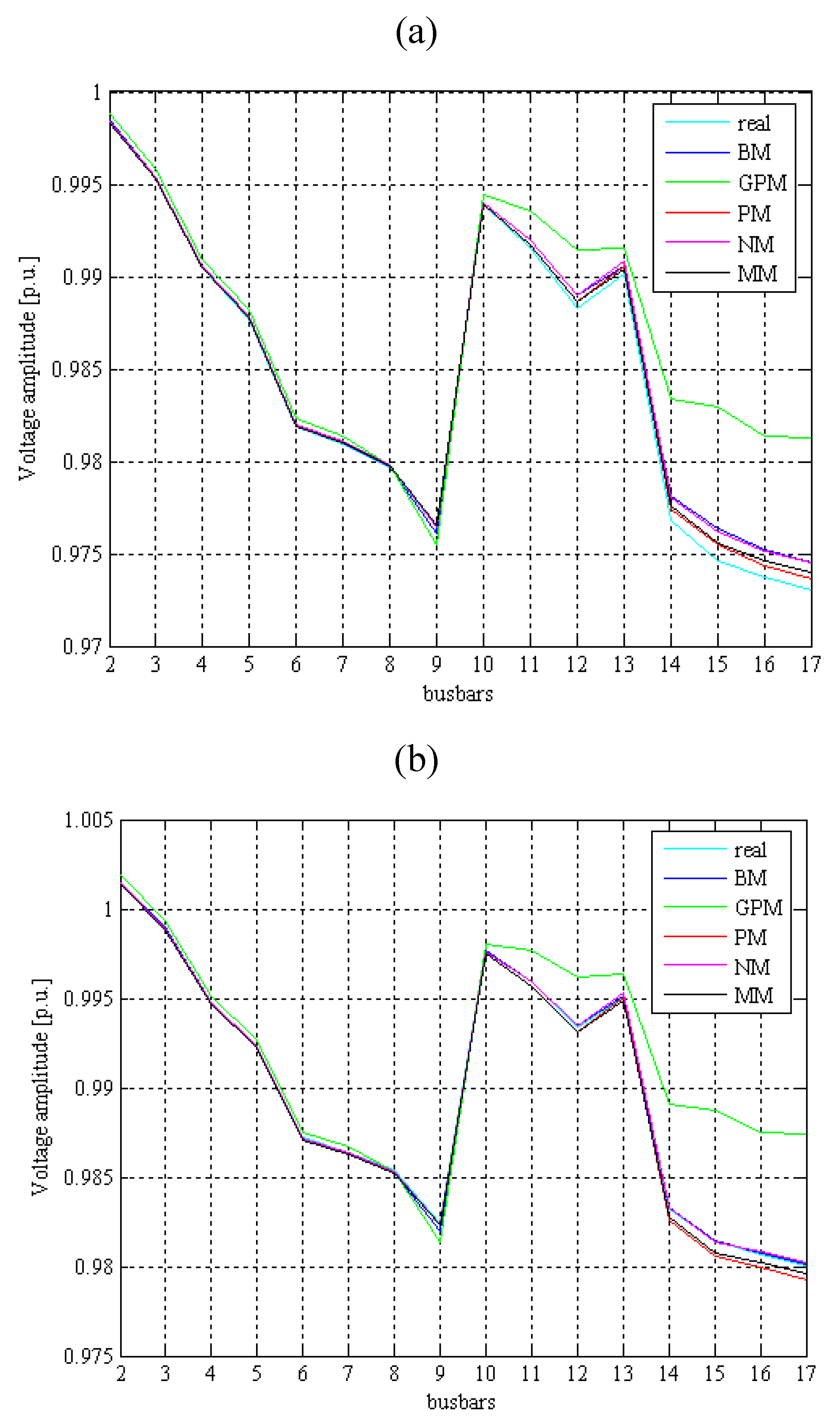
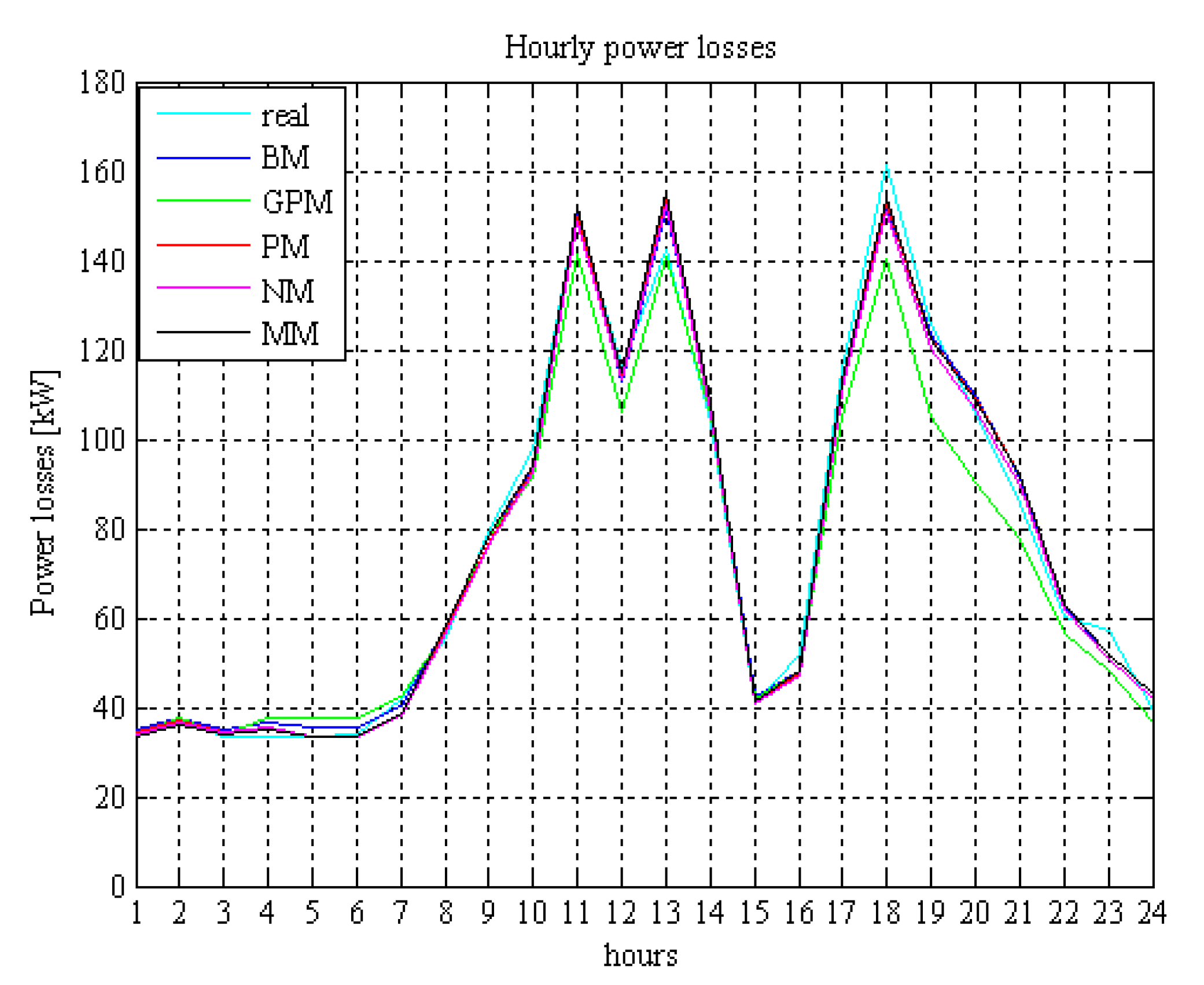
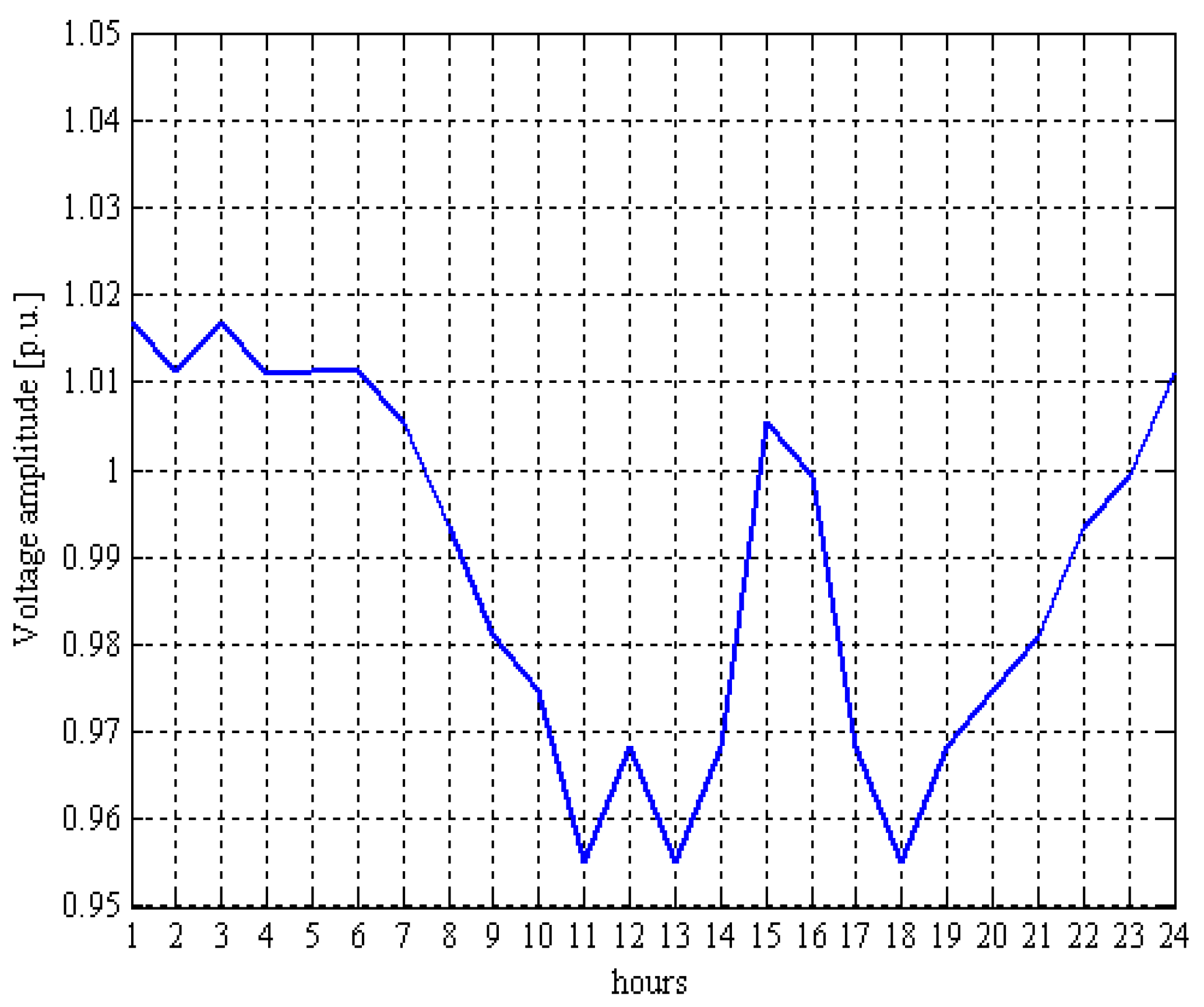
• The steady-state analysis of a distribution system is mandatory in order to determine the voltage profile and the losses, which are strongly influenced by the presence of the wind farm.
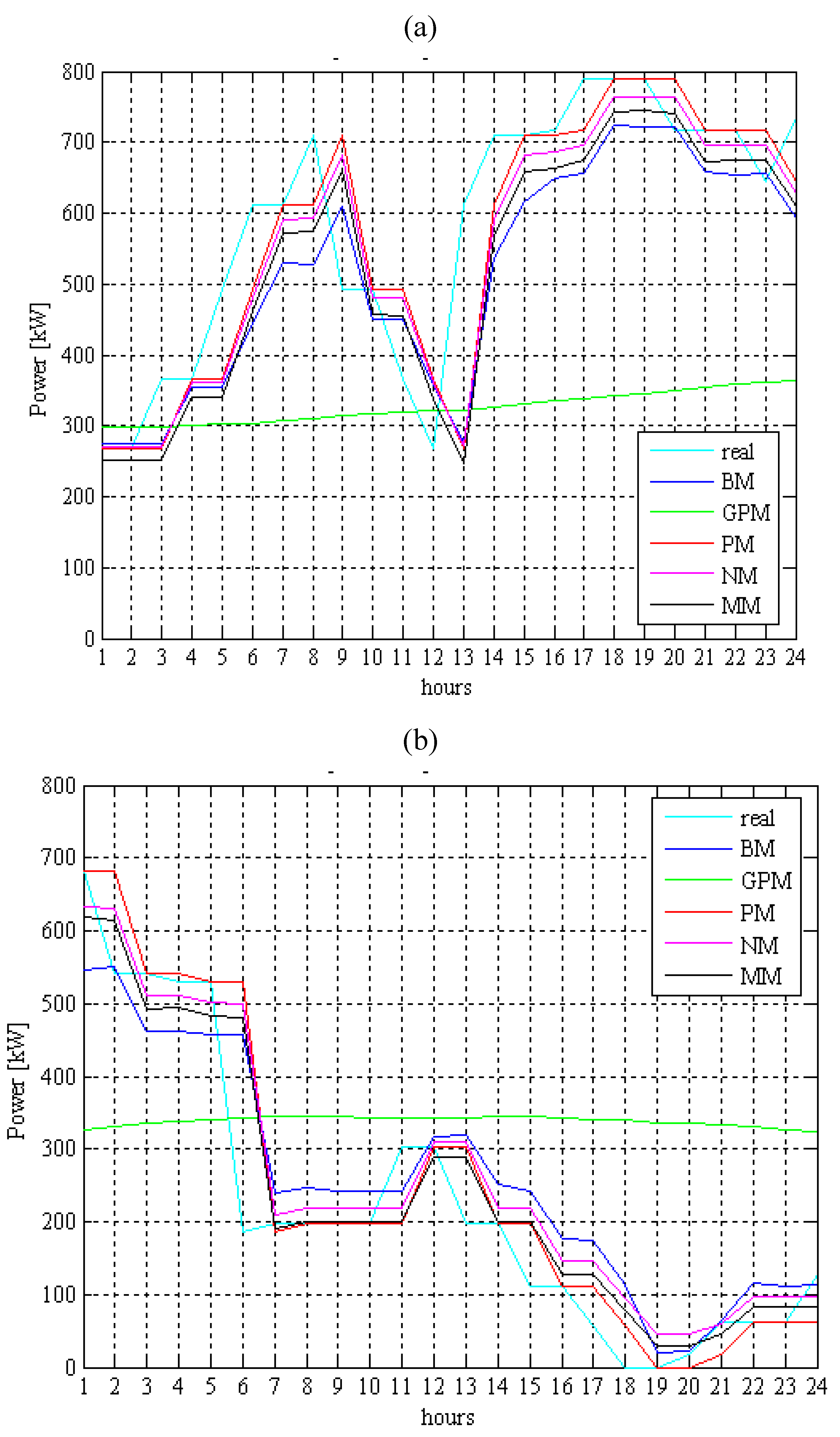
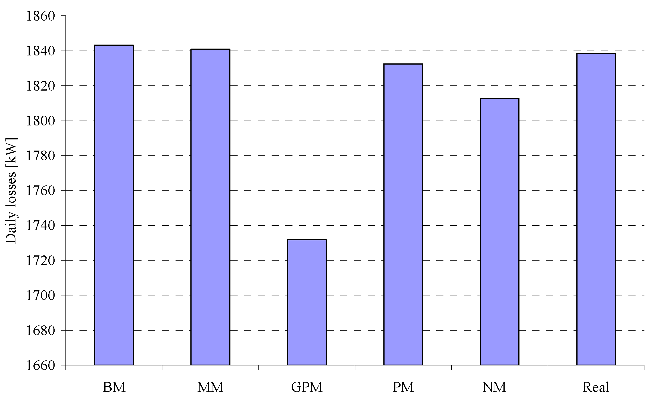
• All wind-forecasting methods, with the exception of the Generalized Persistence Method, furnished similar acceptable results in terms of both voltage profile and losses.
• In the case of the probabilistic approaches, the mean value seems to be the most reliable statistical figure to take into account.
• Probabilistic approaches seems to be the most useful, since they are capable of taking into account the unavoidable time-varying nature of wind speed and of the loads on the steady-state behavior of the distribution system.

References and Notes

1. Smith, J.C. Winds of change. IEEE Power Energy 2005, 3, 20–24. [Google Scholar] [CrossRef]
2. Ahlstrom, M.L.; Zavadil, R.M. The role of wind forecasting in grid operations and reliability. In Proceedings of IEEE/PES Transmission and Distribution Conference and Exhibition, Asia and Pacific, Dalian, Liaoning, China, 23–25 August 2005.
3. De Meo, E.A.; Grant, W.; Milligan, M.R.; Schuerger, M.J. Wind plant integration. IEEE Power Energy 2005, 3, 38–46. [Google Scholar] [CrossRef]
4. Costaa, A.; Crespob, A.; Navarroa, J.; Lizcanoc, G.; Madsend, H.; Feitosa, E. A review on the young history of the wind power short-term prediction. Renew. Sustain. Energy Rev. 2008, 12, 1725–1744. [Google Scholar] [CrossRef] [Green Version]
5. Bracale, A.; Carpinelli, G.; Mangoni, M.; Proto, D. Wind power forecast methods and very short-term steady-state analysis of an electrical distribution system. Elec. Eng. Res. Rep. 2009, 1, 1–8. [Google Scholar]
6. Feijòo, A.E.; Cidràs, J. Modeling of wind farms in the load flow analysis. IEEE Trans. Power Deliv. 2000, 15, 110–115. [Google Scholar] [CrossRef]
7. Giebel, G.; Brownsword, R.; Kariniotakis, G. The state-of-the-art in short-term prediction of wind power. A Literature Overview, 2003. Riso National Laboratory Publication: Denmark. Available online: http://anemos.cma.fr (Accessed on 23 March 2010).
8. Nielsen, T.S.; Joensen, A.; Madsen, H. A new reference for wind power forecasting. Wind Energy 1998, 1, 29–34. [Google Scholar] [CrossRef]
9. Mc Calley, J.; Zhang, J.; Pu, J.; Stern, H.; Gallus, W. A Bayesian approach to short term transmission line thermal overload risk assessment. IEEE Trans. Power Deliv. 2002, 17, 770–778. [Google Scholar] [CrossRef]
10. Bracale, A.; Caramia, P.; Carpinelli, G.; Varilone, P. A probability method for very short-term steady state analysis of a distribution system with wind farms. Int. J. Emerg. Elec. Pow. Syst. 2008, 9, 5. [Google Scholar]
11. Masters, C.L.; Mutale, J.; Strbac, G.; Curcic, S.; Jenkins, N. Statistical evaluation of voltages in distribution systems with embedded wind generation. IEE Proc. Generat. Transm. Distrib. 2000, 147, 207–212. [Google Scholar] [CrossRef]
12. Papaefthymiou, G.; Klockl, B. MCMC for wind power simulation. IEEE Trans. Energ. Convers. 2008, 23, 234–240. [Google Scholar] [CrossRef]
13. Amada, J.M.; Bayod-Rújula, Á.A. Wind Power Variability Model: Part I-Foundations. In Proceedings of the 9th International Conference on Electrical Power Quality and Utilization, Barcelona, Spain, October 2007.
14. Conlon, M.F.; Mumtaz, A.; Farrell, M.; Spooner, E. Probabilistic Techniques for Network Assessment with Significant Wind Generation. In Proceedings of the 11th International Conference on Optimization of Electrical and Electronic Equipment (OPTIM), Brasov, Romania, May 2008; pp. 351–356.
15. Divya, K.C.; Nagendra, R.P.S. Models for Wind Turbine Generating Systems and Their Application in Load Flow Studies. Elec. Power Syst. Res. 2006, 76, 9–10, 844–856. [Google Scholar]
16. Bracale, A.; Carpinelli, G.; Di Fazio, A.; Russo, A. Probabilistic Approaches for Steady State Analysis in Distribution Systems with Wind Farms. In Handbook of Wind Power Systems: Operation, Modeling, Simulation and Economic Aspects; Pardalos, P.M., Pereira, M.V.F., Rebennack, S., Boyko, N., Eds.; Springer; in press.
17. Chang, W.K.; Grady, W.M.; Samotji, M.J. Meeting IEEE-519 harmonic voltage and voltage distortion constraints with an active power line conditioner. IEEE Trans. Power Deliv. 1994, 9, 1531–1537. [Google Scholar]