1. Introduction
With the increasing level of global economic integration and the development of financial market, in the crude oil markets we have seen a more volatile as well as more integrated environment [
1,
2]. On the one hand, the market is influenced by increasingly complicated factors, aside from the fundamental causes such as the basic supply and demand relationship. This is exemplified by the recent intensifying financial crisis, which brought higher level of fluctuations as observed in the crude oil markets. The traditional risk measurement tools such as standard deviations and equilibrium analysis can no longer provide sufficient level of risk coverage when potential risk sources are increasingly differentiated and transient data behaviors are more prevalent. On the other hand, markets across the world are increasingly integrated with the development in both its technological infrastructure and deregulation wave. This is also evidenced from the high level of correlations between both WTI and Brent markets crude oil portfolio forms indispensable part of investment decision making process in the crude oil markets. When the multi-asset portfolio is constructed to reduce the risk level through diversification during portfolio allocation, the reliable and accurate risk measurement for the portfolio is essential for the portfolio management and risk management and affects critically the portfolio performance.
Although the risk measurement research in the crude oil markets has drawn significant research attempts over years, majority of innovative research methodologies are developed for the risk measurement for single asset portfolio. Till now there is only limited attempts to explore various theoretical and empirical issues for portfolio VaR estimation in the literature. One reason is that compared to the numerous attempts to model univariate time series, researches directed toward the understanding and modeling of multivariate time series are much more restricted due to the level of technical difficulties involved. Another reason is that portfolio VaR needs to deal with further complication of modeling second moments including correlation and covariance matrix among multiple assets than the single asset VaR, which involves exponentially increasing level of computational complexity. Typical models used in this field include the much restricted Exponential Weighted Moving Average (EWMA) and the multivariate VARMA-GARCH model for portfolio risk measurement.
Meanwhile, the wavelet based approach is also gaining momentum in the economics and finance literature [
3,
4,
5]. Firstly, wavelet analysis has been used to identify time varying behaviours of market behaviours, key economic variables and their correlation evolutions. A typical example would be the studies on multi-scale price movements and lead lag relationships in various financial markets [
3,
6,
7,
8,
9,
10]. Empirical studies in these markets reveal the multi-scale structure of prices and evolution of their correlation. Secondly, wavelet analysis is used to smooth data at finer scales. As the magnitude of noise is time varying and the signal to noise ratio (
i.e., the threshold level set for the distinction) may be subject to investors’ preferences, data smoothness would improve if smoothing is conducted at a finer time scale domain, and thus improved model fitness and performance would result. Empirical studies based on wavelet shrinkage techniques in both electricity and foreign exchange markets have confirmed the potential performance improvement. For instance, Meng
et al. [
11], Amjady and Keynia [
12] and Aggarwal
et al. [
13] based their neural network forecasting model on wavelet pre-processed data series and obtained positive performance improvement [
11,
12,
13]. Thirdly, wavelet analysis has been used to decompose data series for a finer level of modelling accuracy. Decomposed data series at lower scales are considered dominated by trends and are modelled using econometric approaches. Decomposed data series at higher scales are considered mostly dominated by price volatilities and are modelled using time series approaches. Results of experiments in several energy markets have confirmed the performance improvement [
14,
15]. For instance, Xu
et al. [
16] attempted to combine wavelet analysis with support vector machine and obtained positive performance improvement in empirical studies on the Australian electricity market [
16]. Conejo
et al. [
17] combined wavelet analysis and ARMA model to analyze the Spanish electricity market and obtained positive results [
17].
In the crude oil forecasting and risk measurement literature, we have only witnessed limited efforts. Most of them are accumulating quite recently. These attempts mostly use the wavelet analysis to pre-process the data before time series techniques and machine learning techniques are used to analyze the data and make forecasts. For instance, Yousefi
et al. [
15] used wavelet analysis to decompose crude oil price and extended them directly to make forecasts [
15]. de Souza e Silva
et al. [
18] uses wavelet analysis to remove high frequency noises, then uses HIdden Markov Model (HMM) to predict future price movement [
18]. Naccache [
19] uses wavelet analysis analyze the relationship between macroeconomic conditions proxied by Morgan Stanley Capital International (MSCI) and the crude oil price at finer scales [
19]. We have conducted some exploratory studies on multi-scale based risk measure estimates. He
et al. [
20] used the Morphological Component Analysis with wavelets as bases to investigate the heterogeneous market microstructure [
20]. But the literature on the forecasting aspects of crude oil price is limited to this extent so far.
Meanwhile, risk measurement in the crude oil markets remains another important research topic, but has received much less attention compared to the progress made in the forecasting field. Most of current approaches use the multi-resolution analysis capability of wavelet analysis to look into the past price or correlation behaviours in the capital markets [
21,
22], e.g., it has been used to analyze the risk distribution across differences the scales [
23,
24,
25,
26,
27,
28,
29,
30]. Some researches such as that by Karandikar
et al. [
31] has gone a step further to estimate VaR with this information taken into account. VaR estimated following the traditional approaches is adjusted by the proportion of risks that corresponds to the investment time horizon [
31]. These approaches are unique in that VaRs are tailored to investor’s investment profile [
24]. However, backtesting these VaR estimates may involve additional complexities. Unless risks at all levels are taken into account, using these adjusted VaRs to calculate VaR exceedances may result in the underestimated exceedance levels. The reliability may also be statistically overestimated as a result. Aside from the backtesting issue, the performance of these approaches is also constrained by the accuracy of the traditional methodology used. Thus, when it comes to models’ reliabilities and accuracies, these approaches are more useful as risk analysis tool than methodologies that bring further performance improvement. Recently He
et al. [
32] used wavelet analysis to analyze the risk structure and construct the VaR estimation algorithm based on it [
32]. It is univariate in nature and not directly applicable to the much more complicated multivariate environment. The risk measurement literature is limited to this extent so far concerning the portfolio risk measurement in the multi-scale domain.
Therefore, this paper proposes a novel multivariate wavelet denoising approach for estimating Value at Risk for portfolio in the crude oil markets. Following Heterogeneous Market Hypothesis (HMH), it is assumed that the underlying DGPs vary in their scales, corresponding to different scales of investment. Thus taking different investment scales (i.e., portfolio sizes) as the discriminatory factor, wavelet based denoising algorithm is used to gain insights into heterogeneous market structures categorized roughly on scales of investment. In this paper, we introduce the multivariate wavelet analysis in higher dimensional space to analyze the second moments evolution of crude oil portfolio data. The introduced multivariate wavelet denoising methodology is then used to extract data of distinct characteristics, which are modeled further incorporating the Multivariate GARCH (MGARCH) framework.
The theoretical motivation for the present research is that recognizing these complicated and heterogeneous nature of the crude oil markets, there exists diverse patterns of behavior of different participants, which is the target for the separation and extraction process. These participants need to be categorized and separated from the original data based on their unique behavioral patterns, resulting from different investment horizons and strategies. For example, the behavior of noise traders are temporal and nonlinear, usually resulting from highly speculative behavioral patterns, while the behavior of fundamental investors are characterized with features subject to the extensive studies over years, including auto correlation, heteroscedasticity, mean reverting and long memory, etc.
The practical and technical motivation for the present research is that the challenge to improve estimation reliability and accuracy has been difficult to improve beyond the traditional EWMA and MGARCH models. Recent empirical researches suggest that this is due to its complicated and nonlinear data nature, compared to the linear assumptions adopted before. Besides, crude oil markets typically represent a more volatile and risky environment than the traditional financial markets and demonstrate unique characteristics due to several reasons. Firstly, crude oil is traded less frequently than equities. There are considerable transaction and opportunity costs involved, resulting in higher levels of fluctuations and relatively lower levels of efficiency. Secondly, price movements in crude oil markets are frequently influenced by numerous factors, such as weather conditions, political stability, economic prospects, consumer expectations and business indicators, etc. The complex dynamics involved exhibit multi-scale non-linear characteristics, which are beyond explanatory capabilities of current models and methodologies for forecasting and risk measurement purposes. Despite its significance, forecasting of crude price and the measurement of risk in crude oil markets have not received sufficient attentions, as compared to equities markets. Research in this paper attempts to address the unique characteristics of crude oil markets when constructing useful models for forecasting and risk measurement purposes and to fill the gap in the relevant literature. Meanwhile, wavelet denoising in higher dimension involves directional projection of time series, i.e., multivariate time series can be projected into different directions, normally vertical, horizontal and diagonal. Projections into different directions are associated with different correlations among time series at different time lags.
The key findings and contributions include the following aspects. There have been limited attempts in the literature to model the conditional correlations among portfolio using multivariate GARCH model [
33,
34]. The most related one is Vacha and Barunik [
35]. However, it ignores the dependence structure among portfolio assets, which can only be investigated in the higher dimension. Besides, it does not deal with the utilization of these time varying correlation information into the modeling of risk evolutions, which this paper addresses using the DCC model in the multi-scale framework. Meanwhile, most research focuses on the single variate VaR estimation, among which the most related one is Cifter [
36] that is mainly based on univariate wavelet analysis. This paper instead introduces multivariate wavelet analysis in the estimation of portfolio Value at Risk. Few studies in the literature have investigated the the portfolio risk measurement with time varying correlation. Work in this paper represents one of few attempts to investigate the estimation of portfolio VaR using multivariate wavelet based techniques.
The rest of the paper proceeds as follows:
Section 2 provides a brief account and also literature review on the relevant theories used to construct the proposed algorithm. This includes the portfolio value at risk, multivariate GARCH models and multivariate wavelet analysis theories.
Section 3 proposes the multivariate wavelet denoising approach for estimating portfolio value at risk, with detailed economic rationale explained and numerical procedures. The performance of the proposed algorithm against benchmark alternatives are evaluated in
Section 4. The empirical studies are conducted in the benchmark US WTI and Europe Brent markets and experiment results are reported to justify the superiority of the proposed algorithm.
Section 5 provides some concluding remarks.
3. Multivariate Wavelet Denoising Model for Portfolio Value at Risk Estimates
In the mainstream literature the Efficient Market Hypothesis (EMH) underpins most econometric models in the crude oil markets, which depicts the market structure and price behavior based on the assumption of homogeneous agents with rational expectations and single time horizon. This approximates the market well when there is relatively stronger control and much regulations in place. However, with the deregulation waves, more empirical researches suggest that the market exhibits diverse individual characteristics not just in the frequency domain, but over multi-scale time horizons. Thus the Heterogeneous Market Hypothesis (HMH), initially proposed in the exchange rate and equity market, is proposed in this paper to complement the traditional EMH and recognize these new empirical stylized facts [
72,
73,
74,
75,
76,
77,
78,
79,
80].
HMH can be viewed as a more restricted form of FMH, focusing on heterogeneous features of market microstructure, which comes natural when the market has fractal characteristics. It also complements the traditional EMH [
74,
75,
76,
77,
78,
79,
80]. It assumed that different actors in the heterogeneous market have different time horizons and dealing frequencies. The market is heterogeneous with a fractal structure of time horizons as it consists of short-term, medium-term and long-term components. Different actors are likely to settle for different prices and decide to execute their transactions in different market situations. In other words, they create volatility. The market is also heterogeneous in terms of geographic locations of the participants. Based on these assumptions, the HMH postulates that the market consists of heterogeneous agents with heterogeneous investment strategies and investment time horizons. Compared with the homogeneous reaction to the news shocks in the EMH, HMH states that these agents or investors react to news shocks differently based on their own characteristics. On one hand, their investment time horizon and dealing frequency are diversely different. Their time scale behaviors could range from short and temporal to long and stable characteristics. For instance, pensions funds and central banks tend to have low dealing frequency focusing on long time horizon while the market traders tend to have high dealing frequency with short time horizon. On the other hand, these agents or investors employ diversely different investment strategies or measures based on their own characteristics and focus. Their frequency behaviors could range from stationary to transient characteristics.
In the literature, these micro market structures were studied incorporating information at the operational and transaction level. However, results from these studies are constrained by the restricted access to the concerned data, some insider in nature. The data obtained are also significantly lagged in time due to the regulations on protection of sensitive information. Thus it would be difficult to test the theory and implement it for real time trading environment.
Meanwhile, a different alternative is to use the time series itself without dependence on unreliable external information to extract and separate the underlying components from the original data directly. Certainly it is a difficult problem as the underlying components are unknown latent variables, whose structures are vulnerable to inappropriate separation processes. The multivariate case is made even more complicated by the time varying correlations. The wavelet based approach is promising as it is supported by positive results for decomposing and denoising of univariate time series. However, using wavelet to denoise and separate data features in multivariate time series involves further complications that deserve further investigations.
Therefore, in this paper we propose a different approach to extract and separate the underlying components from the original data directly.
Since the accuracy of the noise and denoised data separation and extraction process affects critically the generalizability of the models fitted, appropriate tools need to be selected. Traditional data denoising techniques include spectrum analysis methods such as simple averages, Kalman filtering and Fourier transforms, etc. However, these methods did not receive significant attentions in the mainstream empirical research literature. This is due to the insignificant performance improvement during the application of these approaches, as they are mostly based on spectrum and frequency scale domain while ignoring the multi-scale heterogeneous structure in the data. More specifically these approaches would result in two critical issues: Firstly, the data may be distorted during the denoising process due to the single time horizon approach, and there are patterns left in the noises removed, which would reduce the forecasting accuracy if ignored. The denoising algorithm with different parameters further complicate this situation. Secondly, following HMH, the noises may vary in level in the multi-scale domain for multi-scale data structure, corresponding to different investment strategies and time horizon. To tackle these issues, the analysis and modeling of the individual components behaviors, including both the separated denoised data and noises, in the multi-scale domain need to be conducted during the denoising process, as it would reduce the risk of using biased estimates with lower goodness of fit and contributes to the overall performance improvement. For example, the behavior of transient data component is significantly different from the behavior of data component driven by normal market activities. Each of them need to be modeled separately to avoid the biased estimate due to violations of assumptions of the unsuitable models.
Thus the wavelet based denoising algorithm is proposed to serve as a promising alternative modeling tool to extract heterogeneous data features of distinct characteristics, in a real time manner without the need of insider information. This is a more refined approach compared with the normal spectrum or frequency domain approach taken by traditional data denoising techniques such as spectrum analysis methods, e.g., simple averages, Kalman filtering and Fourier transforms, etc.
Applying the wavelet based time frequency analysis in the higher dimensions, a two stage Multivariate Wavelet Denoising Portfolio Value at Risk Model (MWDNPVaR) is proposed to track portfolio risk evolution in the higher dimensions space and estimate portfolio VaR.
Accordingly the numerical procedure for the two stage hybrid estimation process is listed as follows.
In the first stage, the multivariate wavelet analysis based denoising algorithm is used to separate the noises matrix from the original data matrix, leaving the rest data matrix with more distinct characteristics.
Then the multivariate time series models are used to extract the denoised and noise matrix respectively, resulting in different model parameters tuned for distinct data characteristics and dependency structure.
In the second stage, since we assume that the denoised and noise data are independently distributed, the conditional means are aggregated from the individual conditional mean forecast matrix forecasted for both denoised and noise data components as in (19).
where
is the aggregated conditional mean forecast at time
t,
and
are conditional mean forecasts for both denoised and noise data respectively, at time
t.
As the wavelet decorrelates the data series, suppose data series across different scales are independent. Thus the variance-covariance matrix can be aggregated from the individual variance-covariance matrix forecast at different scales as in (20).
where
is the aggregated conditional variance-covariance forecast matrix at time
t,
and
are conditional variance-covariance forecast matrix for both denoised and noise data respectively, at time
t.
is the covariance matrix at time
t,
and
.
Then, suppose a unit worth portfolio investment with
ω weights and one day holding period with the forecasted conditional mean and covariance matrixes, we follow the traditional variance-covariance approach for estimating portfolio
as in (21).
4. Empirical Studies
4.1. Data and Descriptive Statistics
Empirical studies are conducted in the US West Texas Intermediate (WTI) and Europe Brent markets, which are the marker markets where most trading and transactions are conducted. Together they form essential part of the crude oil portfolio. The data source is the Energy Information Administration, Department of Energy, US. The data set covers the same date range from 2 January, 2002 to 1 October, 2009 for both markets. The starting date for the data set is chosen since the equilibrium price level has shifted to a new regime since 2002. The potential cause is that the balance between the demand and supply of crude oil is increasingly constrained by its limited and scarce nature in recent years, due to the increasing demand and steady level of supply, as well as the wave of liberalization and globalization. Meanwhile, this time period would reduce the impact of previous direct systematic market disruptions such as the Gulf war, the minimum. The end date for the data set is chosen based on data availability. However, this results in different number of daily observations for each market respectively, i.e., 1939 for WTI market and 1996 for Brent market, as normal trading are interrupted at different time points due to different trading regulations and holidays. For the purpose of constructing a valid portfolio in both market, only observations for the valid trading days in both markets are retained in the data set, i.e., if trading in either one market is disrupted with holiday or regulations, observations for this day are excluded in both markets as no valid portfolio can be constructed. This results in 1939 observations. We assume a one dollar investment portfolio with equal holding positions, i.e., 50% in the WTI market and another 50% in the Brent market. The data set is divided into three subsets, i.e., the training set for determination of model parameters (40%), the model tuning set to select and determine the empirically optimal model specifications (20%) and the test set for the out-of-sample test to evaluate the performance of different models (40%). This results in 776 daily observations for out-of-sample test, yielding statistically significant results. The one day ahead forecast is performed using rolling-window method. The size of the window is 775 to cover the relevant information available. As autocorrelation and partial autocorrelation function indicates the trend factors, the daily prices are log differenced at the first order to remove them as in . We assume one day holding period to conduct one step ahead PVaR estimations.
The descriptive statistics for both markets are listed in
Table 1.
Table 1.
Descriptive statistics and statistical tests.
Table 1.
Descriptive statistics and statistical tests.
| Data | | | |
|---|
| Mean | 0.0011 | 0.0011 | 0 |
| SD | 0.0227 | 0.0160 0.0160 |
| Skewness | −0.4177 | −0.4975 | 0.0288 |
| Kurtosis | 4.8569 | 6.4738 | 3.2942 |
| JB Test | 0 | 0 | 0.1064 |
| BDS Test | 0.0037 | 0 | 0 |
| Data | | | |
| Mean | 0.0011 | 0.0011 | 0 |
| SD | 0.0219 | 0.0165 | 0.0144 |
| Skewness | −0.1009 | −0.4202 | 0.0069 |
| Kurtosis | 4.3219 | 6.2835 | 2.8970 |
| JB Test | 0 | 0 | 0.5000 |
| BDS Test | 0.6313 | 0 | 0 |
Descriptive statistics in
Table 1 show some interesting stylized facts. On the aggregated level, the distribution of the original data approximates the normal distribution, as indicated by four moments. However, the rejection of the null hypothesis for Jarque–Bera (JB) test of normality suggests the deviation of return distribution from the normal distribution [
81]. The rejection of the null hypothesis for BDS test suggests the existence of unknown correlations, potentially nonlinear dynamics, in the data [
82]. However, compared to descriptive statistics of individually denoised data series in
Table 1, the multivariate denoising algorithms extract correlated denoising data and noises data. The paired data in both markets exhibit similar descriptive statistics, suggesting that they are governed by correlated or the same underlying DGP.
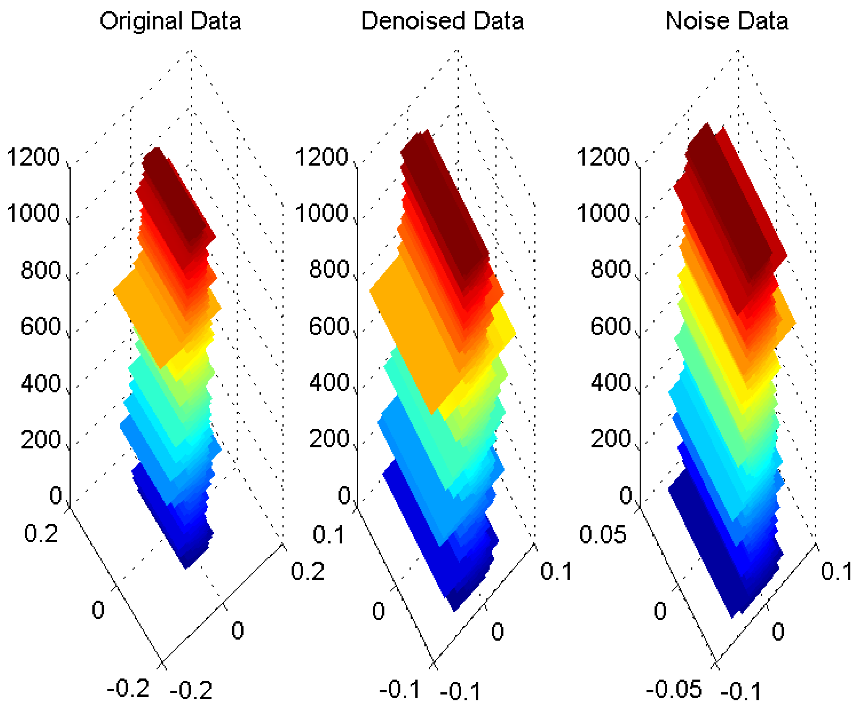
Figure 1 shows the surf plot of return series in both markets.
Results in
Figure 1 show that multivariate wavelet analysis effectively separates data of distinct characteristics and shapes. The middle figure for denoised data show distinctively different shapes and behaviors than the right figure for noise data. Behaviors of both of them are different than the left figure for the original data. Interestingly, these figures show that some of the data features in the left figure are signified in the middle figure while others are signified in the right figure. For instance, the abrupt changes in the left figure are mostly captured in the middle figure.
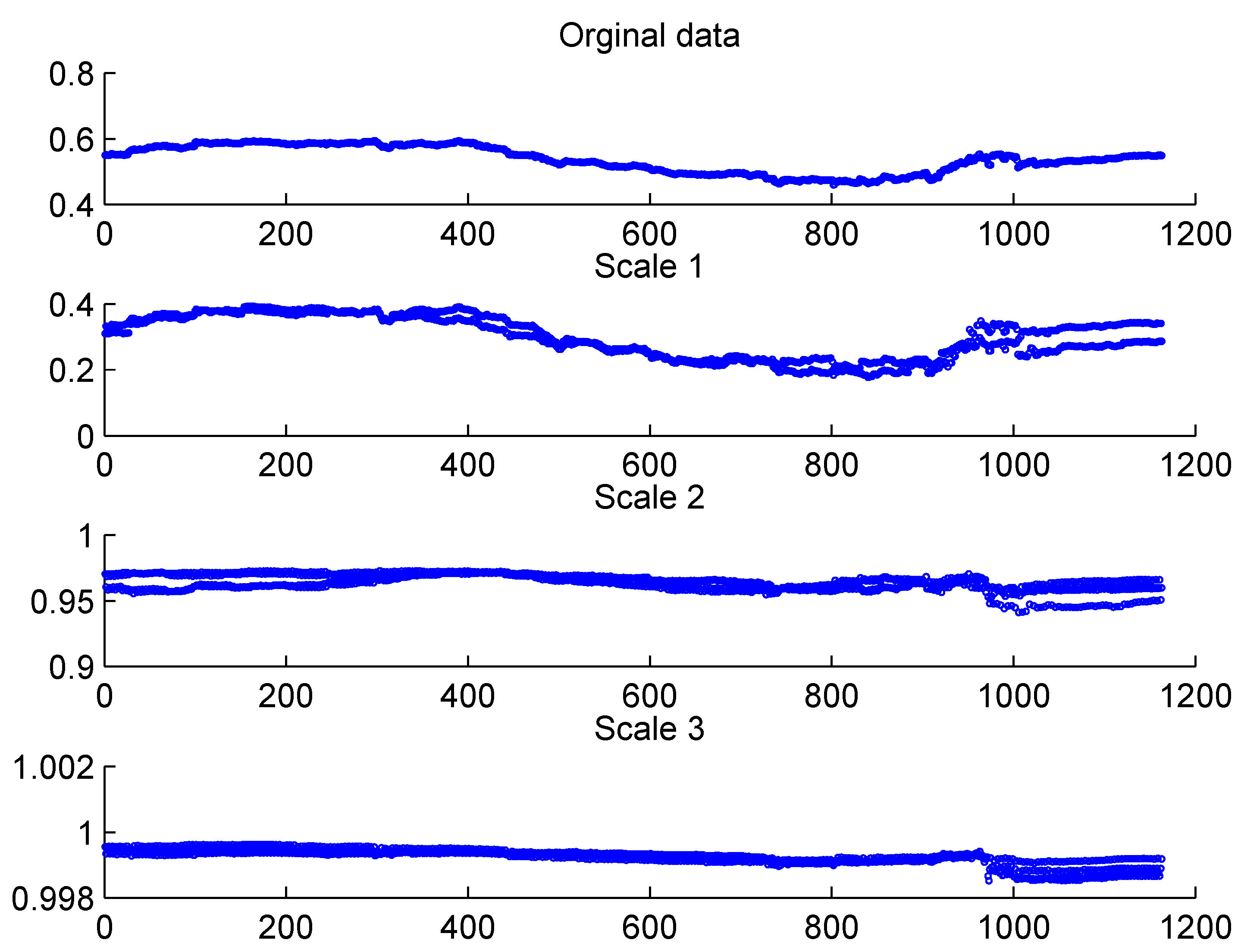
4.2. Multi-scale Analysis of Correlation of Portfolio
As we argue that the correlation between different markets consists of varying strength of correlations at different scales, the cross correlation wavelet analysis is used to analyze and illustrate the multi-scale structure of correlation movements. The rolling windows over which the correlation is calculated is 775. For the portfolio data series decomposed at scale 8 with Daubechies 8 wavelet family, correlation for data series at the first three levels along with the correlation for the original portfolio are shown in the scatter plot in
Figure 2.
Figure 1.
The surf plot of the original, denoised and noise data.
Figure 1.
The surf plot of the original, denoised and noise data.
Figure 2.
Dynamic correlation between WTI and Brent markets at different scales.
Figure 2.
Dynamic correlation between WTI and Brent markets at different scales.
Experiment results in
Figure 2 show that the correlation between WTI and Brent market is dynamically changing over the entire investment time horizon, between 0.44 and 0.6. This justifies the use of DCC-GARCH model, in which the dynamic correlation assumptions better conform to the real data.
Using wavelet analysis, the underlying structure of correlation is recovered when relating the strength of correlation to the investment time horizon. For instance, over the short term investment time horizon, the correlation is relatively low for these particular portion of markets. We also observe strong correlation between particular portion of both markets over the medium to long term time horizon.
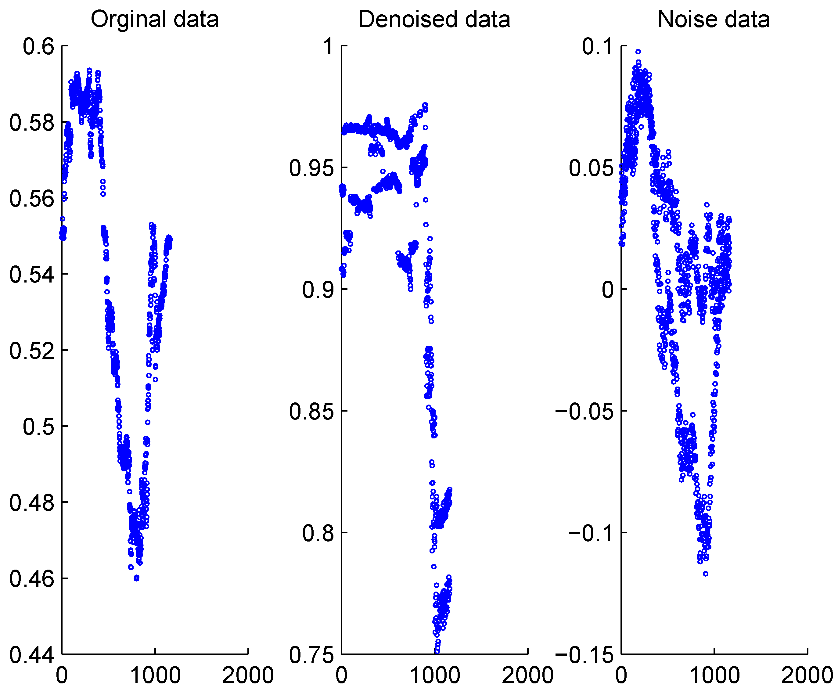
In addition to the multi-scale correlation structure, there are also heterogeneous structure for the correlation evolution,
i.e., the correlation between different markets may be influenced by underlying correlations of different strength and characteristics. Therefore, we further use the cross correlation wavelet analysis to analyze and illustrate the heterogeneous correlation movements. The original, denoised and separated noise correlation between WTI and Brent market are shown in the scatter plot in
Figure 3.
Figure 3.
Dynamic correlation between WTI and Brent markets.
Figure 3.
Dynamic correlation between WTI and Brent markets.
Experimental results in
Figure 3 show that correlation for the extracted denoised data series exhibits time varying behavior at higher range between 0.75 and 0.95, while correlation for the noise data series also exhibits time varying behavior at lower range between −0.15 and 0.1. This shows that under the HMH framework, the multi-scale heterogeneous structure of correlations can be recovered using wavelet analysis to extract dependency structures of distinct nature, which drives the dynamic correlation behaviors. In this case, they are roughly categorized into denoised and noise parts to signify their distinct characteristics. Therefore they need to be modeled using different model specifications and parameters.
These experiments signify the multi-scale and heterogeneous correlation structure as important stylized facts that need to be incorporated during the modeling process. Wavelet analysis based denoising algorithm provides an interesting alternative to uncover the multi-scale heterogeneous correlation structure, by projecting the original data into different time scales and extracting different denoised and noise components at these scales.
4.3. Performance Evaluation
The performance of the proposed MWDNPVaR model is evaluated in the empirical studies in the marker WTI and Brent market, against benchmark models. In this paper, we use two models as benchmark models,
i.e., the well accepted EWMA as the de facto industry standard and DCC-GARCH due to its theoretical superiority. The generalizability of the proposed model models is evaluated against benchmark models in out-of-sample forecast tests, using the Kupiec backtesting procedure for unconditional risk coverage for reliability of estimates as well as MSE and Clark–West test of predictive accuracy for the accuracy of estimates [
83,
84].
The frequency based approach, or the so-called unconditional coverage approach, as suggested by Kupiec, tests the statistical significance of the patterns of VaR exceedance,
i.e., whether the size of the loss is greater than the estimated VaR values. The null hypothesis for the Kupiec test is that the proposed model is the correct one and corresponds to the theoretical risk coverage. If the model is acceptable, the number of tail losses
x should follow binomial distribution. Thus, at the given total number of observations
n and confidence level
p, the likelihood ratio statistics is calculated as in (22):
The Kupiec likelihood ratio test statistics conforms to the distribution.
The Kupiec backtesting procedure is intuitively and computationally appealing. However, it relies entirely on frequency of losses information and ignores temporal pattern of exceedances and the size of losses. Thus, it suffers from lower level of discriminatory power for small sample sizes. Therefore backtesting procedures addressing other loss exceedances patterns are developed such as the one proposed by Christoffersen to test for the temporal behavior of losses [
85]. However, when the sample size is sufficiently large, the Kupiec backtesting procedures would offer an acceptable level of discriminatory power between good and bad models. Therefore, it is adopted in this paper to backtest and evaluate different models.
The MSE is the simple statistics measuring the deviation of forecasts from actual observations, as , where .
Diebold Mariano test of equal predictive accuracy is conventionally used to test the statistical significance of the differences of empirical losses between competing models and benchmark models, based on Mean Squared Prediction Error (MSPE). However, it is found that the originally proposed test statistics is upward biased heavily if models tested are nested. Thus the Clark–West test of equal predictive accuracy is proposed to incorporate this important nested model structure in forecast evaluation problems and adjust for the DM statistics as in (23).
is sample mean while
P is the sample size.
The null hypothesis for the test is: , i.e., equal predictive accuracy or MSPE, for the proposed model against the benchmark models nested. The test statistics has a asymptotically normal distribution.
4.4. Experiment Results
In this study, all models are implemented via the Matlab software package from the Mathworks corporation. As confirmed by numerous empirical studies, the lag order for DCC-GARCH model is set to be 1 and 1 based on the parsimony principle. Since we assume no particular distribution for data and there lacks formal methodology to test the goodness of fit of different wavelet family for the data, we test the in-sample performance of the models with different specifications with the reserved model tuning set to determine model specification. The size of in-sample model tuning set for the selection of model specification is 387.
Table 2 lists the in-sample experiment results for the number of exceedances for MWDNPVaR model with different specifications including scales, wavelet basis and shrinkage algorithm. The number of exceedances for different confidence levels
are listed in the parenthesis as
. The number of exceedances for EWMA and DCC-GARCH model are (1,4,10) and (3,12,18) respectively.
Table 3 lists the
p value of Kupiec backtesting procedure for exceedances observed.
Table 2.
Exceedances for different model specifications.
Table 2.
Exceedances for different model specifications.
| Scale | DB2-H | DB2-S | SYM2-H | SYM2-S | COIF2-H | COIF2-S | DMEY-H | DMEY-S |
|---|
| 1 | (4,12,21) | (3,9,18) | (3,8,20) | (1,8,20) | (3,8,16) | (4,9,14) | (3,13,19) | (2,5,18) |
| 2 | (2,12,29) | (4,12,17) | (3,11,23) | (4,9,22) | (5,11,15) | (4,7,14) | (5,8,20) | (4,6,17) |
| 3 | (5,13,23) | (5,9,14) | (4,10,20) | (4,12,24) | (6,10,20) | (1,2,12) | (2,12,23) | (2,9,20) |
| 4 | (5,8,22) | (5,9,24) | (2,7,17) | (5,7,13) | (9,22,33) | (5,11,25) | (6,10,15) | (1,5,22) |
| 5 | (5,9,16) | (5,14,26) | (1,5,19) | (4,8,18) | (4,11,24) | (4,8,18) | (4,8,18) | (6,12,20) |
| 6 | (2,7,17) | (4,9,19) | (3,6,19) | (2,12,23) | (1,6,16) | (4,11,20) | (3,8,17) | (2,3,13) |
| 7 | (4,13,22) | (3,7,15) | (2,7,20) | (2,4,16) | (0,4,9) | (5,7,16) | (4,11,23) | (5,11,19) |
| 8 | (3,9,14) | (4,10,24) | (4,10,18) | (3,9,14) | (4,6,19) | (3,8,19) | (3,7,24) | (5,10,19) |
| 9 | (5,10,17) | (3,11,20) | (2,6,19) | (5,10,21) | (5,8,19) | (4,13,22) | (1,6,14) | (4,9,27) |
Table 3.
P value of Kupiec backtesting procedure for the range of exceedance values.
Table 3.
P value of Kupiec backtesting procedure for the range of exceedance values.
| N | P | N | P | N | P | N | P | N | P | N | P |
|---|
| 0 | 0.0053 | 4 | 0.0366 | 11 | 0.6728 | 9 | 0.0072 | 17 | 0.5760 | 23 | 0.4078 |
| 1 | 0.0805 | 6 | 0.1987 | 12 | 0.4653 | 10 | 0.0166 | 18 | 0.7501 | 24 | 0.2951 |
| 2 | 0.2924 | 7 | 0.3600 | 13 | 0.3032 | 13 | 0.1162 | 19 | 0.9348 | 25 | 0.2064 |
| 3 | 0.6436 | 8 | 0.5742 | 14 | 0.1864 | 14 | 0.1902 | 20 | 0.8801 | 26 | 0.1396 |
| 4 | 0.9473 | 9 | 0.8240 | | | 15 | 0.2916 | 21 | 0.7041 | 27 | 0.0914 |
| 5 | 0.5807 | 10 | 0.9162 | | | 16 | 0.4211 | 22 | 0.5449 | 29 | 0.0355 |
In
Table 3 ,
refers to the number of exceedances at different confidence levels,
,
refers to
p value of Kupiec backtesting procedure at different confidence levels. Experiment results from
Table 2 show the different in-sample performance for the proposed MWDNPVaR, using different model parameters. The three numbers in the parentheses correspond to exceedances at three different confidence levels,
i.e., 99%, 97.5% and 95%. The attempted model parameters are as follows: 4 different wavelet families including Daubechies 2 (DB2), Symlet 2 (SYM2), Coiflet 2 (COIF2) and DMEY 2. Hard and soft thresholding algorithm. Decomposition levels from 1 to 9. The
p value of backtesting procedure is (0.0805, 0.0366, 0.0166) for the EWMA model and (0.6436, 0.4653, 0.7501) for the MGARCH model. Using exceedances and their associated Kupiec backtesting statistics as performance measure as in
Table 2 and
Table 3, we determine the optimal model specification demonstrating the highest level of reliability, as indicated by the higher
p value for the out-of-sample test,
i.e., Symlet 2 using hard thresholding algorithm at decomposition level 3. The shrinkage algorithm is minimax threshold. The thresholding is conducted in a level dependent manner. The
p value of backtesting procedure for the chosen model is (0.9473, 0.9162, 0.8801).
The reliability performance measure of the proposed algorithm against alternative benchmark models are listed in
Table 4.
Table 4.
Reliability comparison of different models.
Table 4.
Reliability comparison of different models.
| Models | CL | Exceedance | KT |
|---|
| | 99% | 32 | 0 |
| EWMA | 97.5% | 52 | 0 |
| | 95% | 67 | 0 |
| | 99% | 8 | 0.9313 |
| DCC-GARCH | 97.5% | 29 | 0.0395 |
| | 95% | 52 | 0.0383 |
| | 99% | 7 | 0.7804 |
| MWDNPVaR | 97.5% | 20 | 0.8908 |
| | 95% | 39 | 0.9737 |
Experiment results in
Table 4 show that the proposed MWDNPVaR algorithm improves the reliability significantly compared with the traditional EWMA and DCC-GARCH model. The exceedances of the MWDNPVaR algorithm decreases substantially across all confidence levels. This result is statistically significant as confirmed by the significant
p value. We also observed significantly improved
p value at both 97.5% and 95% confidence levels from the Kupiec test statistics.
The performance improvement is attributed to the introduction of multivariate wavelet denoising algorithm as the data separation tool. More specifically, this is mainly attributed to the use of multivariate wavelet denoising algorithm to separate data and noises, taking into account their distinct behavior patterns. It is also attributed to the individual modeling of the separated components in the multi-scale time domain, taking into account the heterogeneous data structure.
We further conduct experiments to investigate the predictive accuracy of the proposed algorithm against benchmark alternatives. Results from experiments are listed in
Table 5.
Table 5.
Predictive accuracy comparison of different models.
Table 5.
Predictive accuracy comparison of different models.
| | | MSE | CW | CW |
|---|
| | 99% | 0.0028 | N/A | 1 |
| EWMA | 97.5% | 0.0022 | N/A | 1 |
| | 95% | 0.0018 | N/A | 1 |
| | 99% | 1.1391 | 1 | N/A |
| DCC-GARCH | 97.5% | 0.8594 | 1 | N/A |
| | 95% | 0.6561 | 1 | N/A |
| | 99% | 18.7991 | 1 | 1 |
| MWDNPVaR | 97.5% | 14.1771 | 1 | 1 |
| | 95% | 10.8310 | 1 | 1 |
Experiment results in
Table 5 show that the proposed MWDNPVaR achieves inferior predictive accuracy than the benchmark EWMA and DCC-GARCH based models, as measured by larger MSE. However, the performance gap is not statistically significant, as shown by the failure to reject the null hypothesis for Clark–West test of predictive accuracy. This implies that the predictive accuracy of the proposed MWDNPVaR model is at the comparable level as the traditional MGARCH based PVaR models in asset allocations and utilization. The main purpose of the downside risk estimate as those presented in this manuscript is to improve the reliability to allow sufficient capital allocation to cover the potential significant capital loss due to adverse market price movement. The proposed algorithm in this manuscript can help to estimate risks more reliably under the turbulent period with the prevalence of transient or extreme events, at the cost of predictive accuracy, if investors are risk averse.
There are some important implications drawn from the empirical investigations in the paper. Firstly, although previous researches show that there are increasingly diversified data features, such as extreme events, that can not be explained by MGARCH models based on normal distribution, our results show that it could be attributed to the heterogeneous structure of the underlying data components, potentially much simpler than previously assumed extreme distribution. Thus based on the parsimony principle, it is inappropriate to disregard MGARCH based models in favor of others, such as the models based on extreme value theories. By deliberately separating and modeling the data and noise, the performance of DCC-GARCH model can be improved further to the competent level. Secondly, the optimal performance is achieved when the individual components are extracted using Symlet 2 wavelet family and modeled with different parameters. These observations support the argument that the risk in the crude oil prices are complicated processes with a mixture of underlying DGPs. Its modeling and analysis is a tricky issue which requires the detailed look into the underlying structure in the time scale domain. Thus appropriate recovery of the underlying structure is critical to the further performance improvement and more thorough understanding of the DGPs during the modeling process.
Results and conclusions are generalizable and are supposed to be valid across different data sets and time windows, i.e., the proposed algorithm is expected to lead to improved reliability since the disruptive noise parts are separated in the multiscale domain.


