Article

Experimentally Based Model to Size the Geometry of a New OWC Device, with Reference to the Mediterranean Sea Wave Environment

ICEA, University of Padova, V. Ognissanti 39, Padova 35129, Italy
*
Author to whom correspondence should be addressed.
Energies 2013, 6(9), 4696-4720; https://doi.org/10.3390/en6094696
Submission received: 5 June 2013 / Revised: 1 July 2013 / Accepted: 19 August 2013 / Published: 9 September 2013
(This article belongs to the Special Issue Energy from the Ocean - Wave and Tidal Energy)

Abstract

:
This note presents the Seabreath wave energy converter, basically a multi-chamber floating oscillating water column device, and the lumped model used to size its chambers, the ducts and the turbine. The model is based on extensive testing carried out in the wave flume of the University of Padova using fixed and floating models with a dummy power take off and indirect measurement of the produced power. A map with the available energy in the Mediterranean Sea is also proposed, showing possible ideal application sites. The Seabreath is finally dimensioned for a quarter scale test application in the Adriatic Sea, with a 3 kW turbine, and a capacity factor of 40%.

1. Introduction

The research and development process of wave energy converters is conveniently organized in stages (see for instance [1]). Basically seven steps are needed: (1) proof of concept, with no relevant measurement system; (2) evaluation of the hydraulic efficiency of the device, a first check in the lab of the device potential in converting energy, with hints to improve the device; (3) a series of specific numerical and experimental studies where the critical issues are pointed out and solved; (4) in situ testing, typically a quarter or 1:10 scale of a device not connected to the electric grid; (5) demonstration phase, where the device is tested at real or 1:2 scale, connected to the grid, and the real economic potentiality are tested; (6) a few experimental installations supported by the government; (7) commercialization.
This note addresses the Seabreath technology, patented in 2008, and now in the process of selecting possible locations for in situ testing at a relatively large scale, approximately 1:10 compared to a tentative full scale design (step 4). This paper describes small scale physical model tests carried out in 2009 and 2010, published under concession of the inventor, Luigi Rubino, and the semi-analytical method used to size the device ducts. The method has turned out to be very handy in several occasions.
The Italian Seabreath device is not well known in the Scientific Community. In [2], an authoritative critical review of wave energy converters around the world is given. Only one of the Italian devices is quoted, the Italian REWEC (e.g., [3,4]), but it is not included in the list of technologies that have been considered to be object of extensive development effort. This is in contrast with the state of advancement of this device, close to commercialization in Italy, with one full scale application now under construction (Marina di Cicerone, Formia, Italy) and two under detailed design (Civitavecchia Port, Salerno Port).
Several other reviews, including the map on the European ocean energy projects published by La Tene Maps, do not include any of the Italian projects.
The reason for this lack of attention to the R&D of all countries facing only the Mediterranean Sea (and for the poor visibility achieved by the participation into international projects) is possibly due to the low energetic content of this sea, that makes the economic harvesting of wave energy unlikely.
Conversely, the Mediterranean Sea is suitable for testing devices of relatively small size compared to prototype and therefore such area favours the development of interesting technologies. Noteworthy Italian patents are discussed in [5,6]. Applications of foreign technologies in Italy are presented, for instance, in [7,8,9].
The amount of wave energy available in Italy has been investigated, among others, by [10,11,12,13], based on the national net for wave monitoring [14]. Only recently [15] proposed an accurate wave energy map, based on MedAtlas data [16], calibrated against wave buoy data. The high quality data used in such paper were used to assess deep water energy flux (see also [17]). Actually, the raw data are available and may be used by any user to find the available energy flux even in shallow water.
To sum up, the aim of the paper is twofold. First, to present a map of the available shallow water wave energy flux within the Mediterranean Sea, based on the data described in [16]. Second, to present a numerical model solving the air flowing along the ducts of a multichamber OWC such as the Seabreath device. The model is used to assess the WEC efficiency (or capture width) with respect to the Italian sea environment.
The wave energy maps are proposed in Section 2, showing the actual amount of energy flux in the Mediterranean and the percentage of calm conditions (wave below 0.5 m), i.e., when the devices can be easily accessed. The Seabreath device is described in Section 3. The device efficiency is investigated on the basis of experimental tests presented in Section 4, and numerical simulations presented in Section 5.
A final example application of a quarter scale device is proposed off-shore Riccione (Adriatic Sea). The device is dimensioned and the expected production is assessed. The location was proposed within the FP7 Project Theseus “Innovative technologies for safer European coasts in a changing climate”, in order to evaluate the coastal protection efficiency of the array of WECs combined to the existing submerged sand bag barriers.

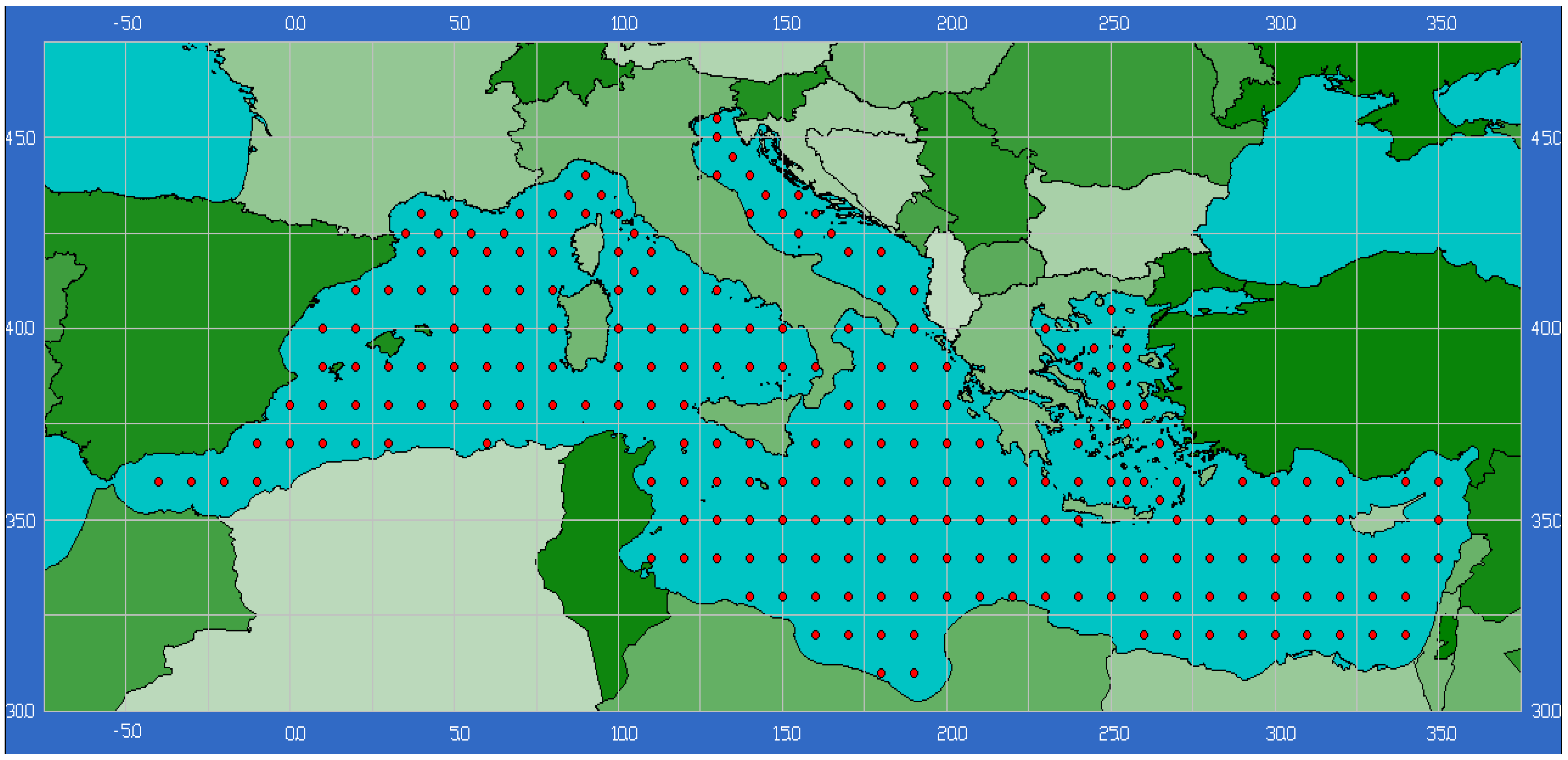
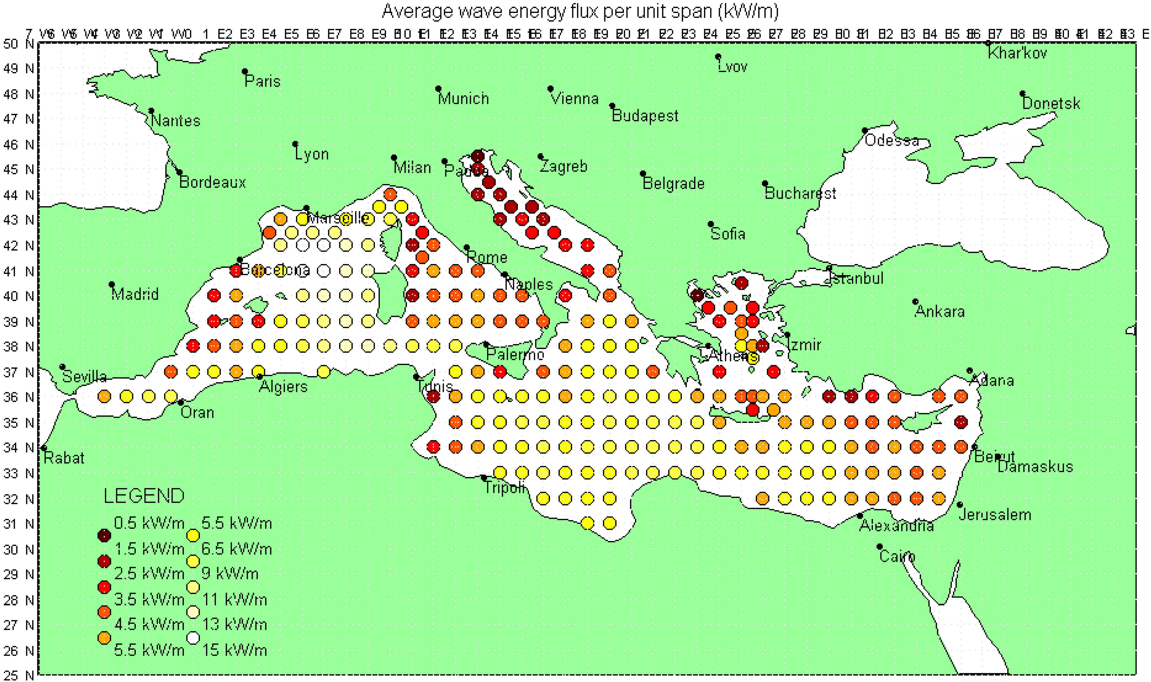
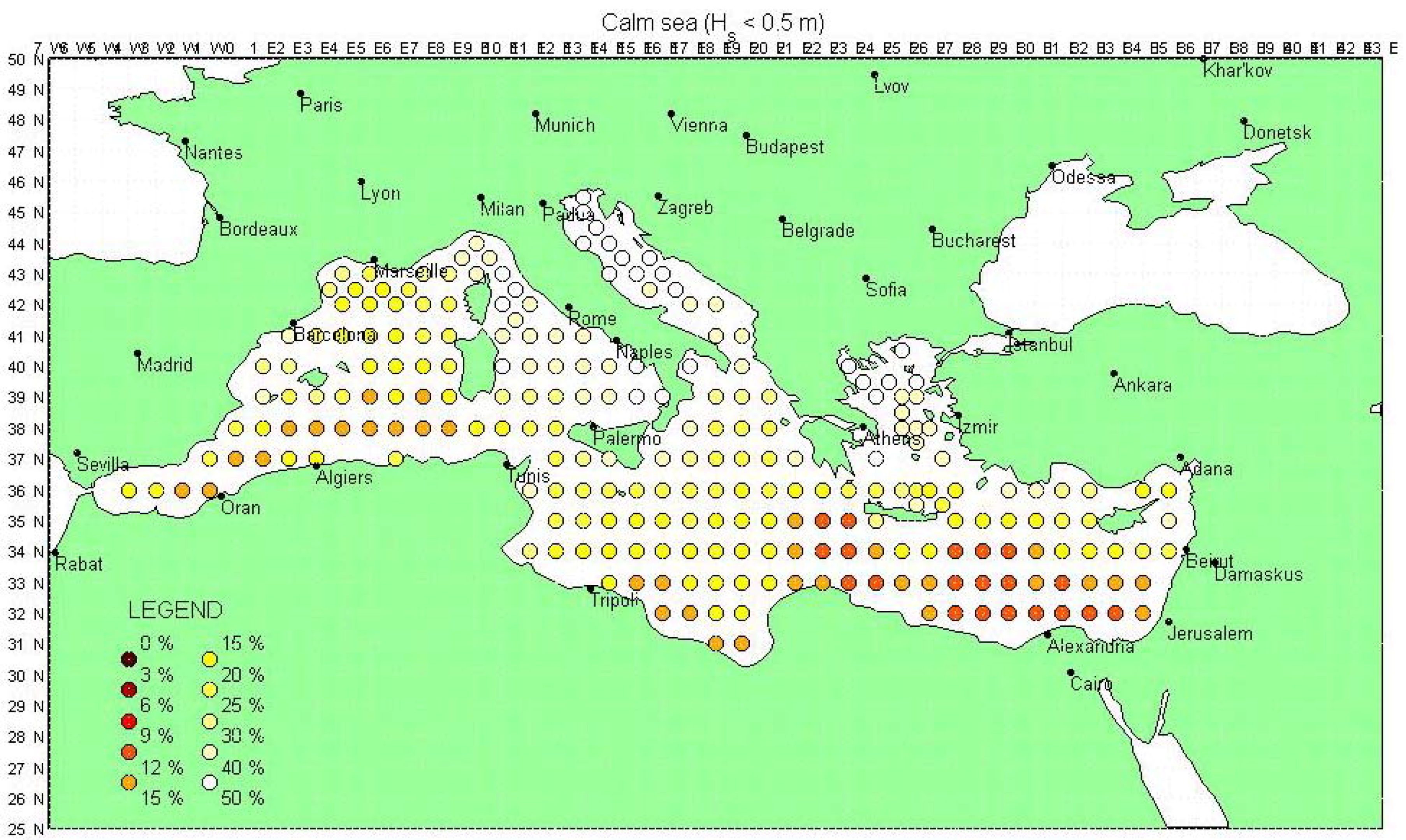
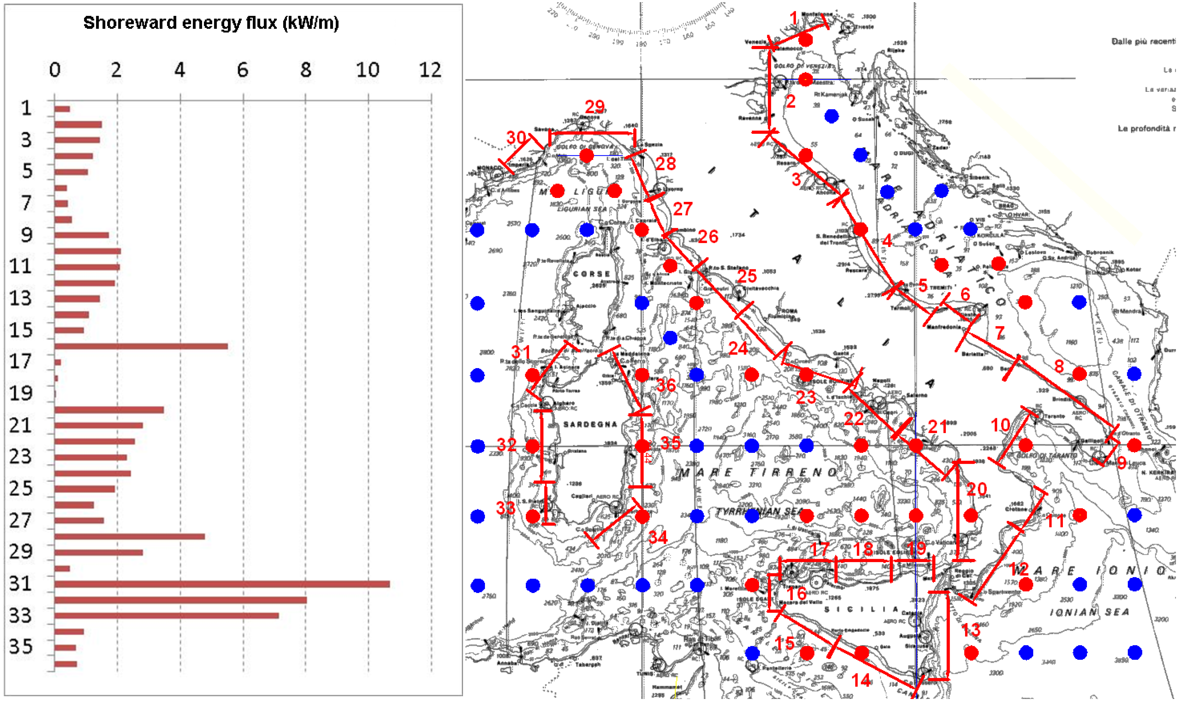
2. Wave Energy Map in the Mediterranean Sea
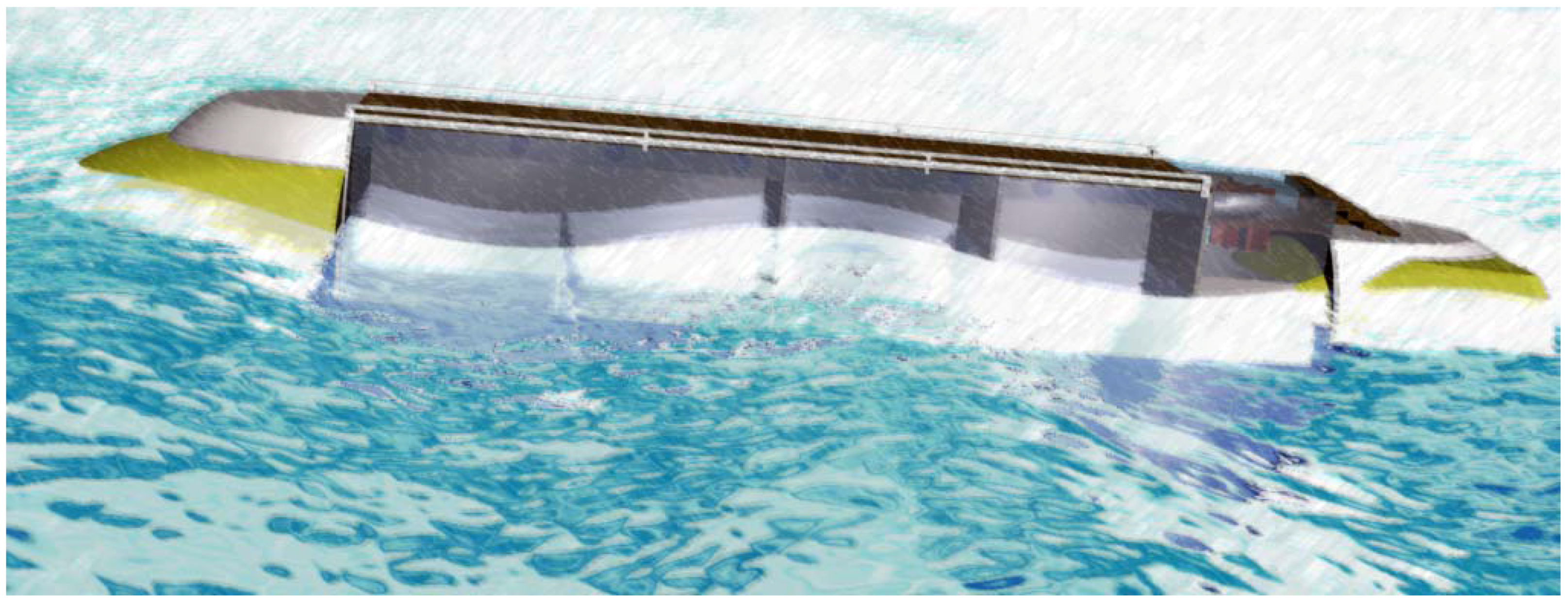
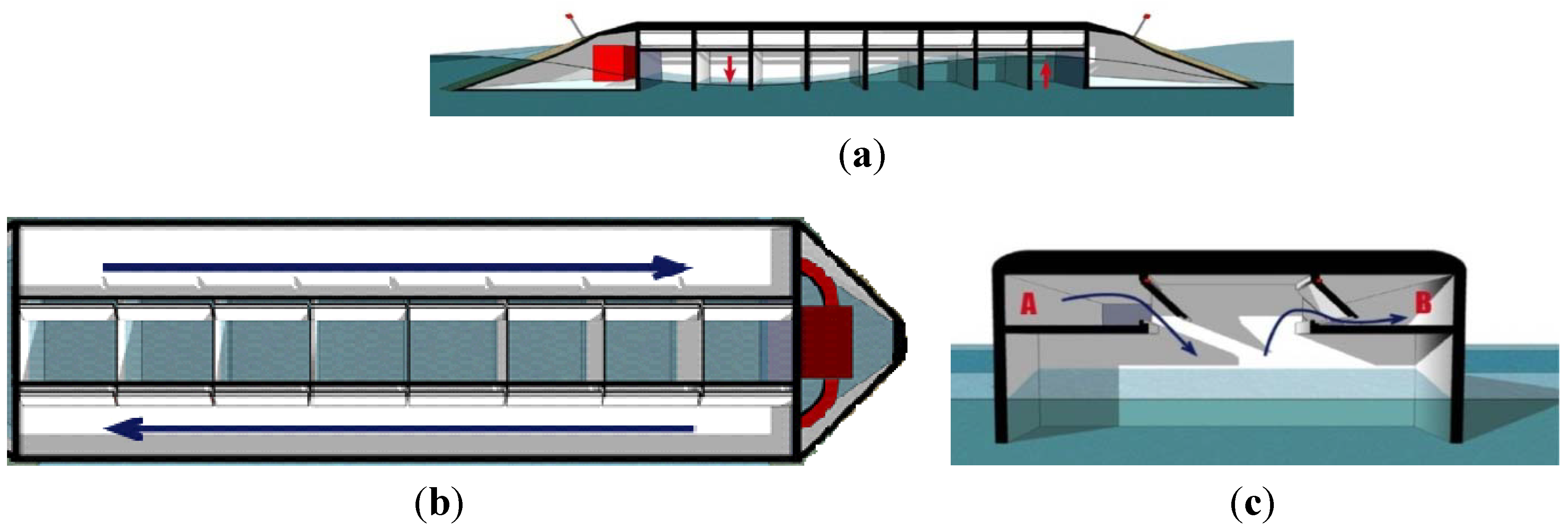
This Section aims at giving a quantitative assessment of the energetic wave potential in the Italian Seas, for possible harvesting with floating wave energy converters.
Data used to integrate the energy flux are obtained from MEDATLAS [15], where the wave climate is given for 239 points, located as in Figure 1. Accuracy of the prediction in the whole Mediterranean Sea is discussed in [18,19].
Figure 1. Map with points where the wave climate is available [15].
Energies 06 04696 g001
For each point, the information obtained from MEDATLAS is the average wave climate in terms of yearly occurrence for classes of wave height (17 values), period (19) and direction (24). The local depth is obtained from nautical charts.
In Figure 2, the energy flux, integrated along all directions, is presented in color scale. Similar maps have already been published in Italian by the Authors [20].
Figure 2. Energy flux per unit span, integrated for all directions.
Energies 06 04696 g002
Figure 3 shows the percentage of time for which the significant wave height is lower than 0.5 m (calm sea condition), i.e., when an ideal floating device would be easily accessible.
Figure 3. Percentage of calm sea conditions.
Energies 06 04696 g003
In order to find the total energy flux in the Italian Seas that may be harvested, a closed curve is drawn around Italy and divided into 36 straight segments. For each segment the following two quantities have been evaluated: (i) the average energy density in a range that may be converted (above 0.5 m and below un upper threshold given by the 0.1% percentile of the frequency of occurrence); (ii) the projected energy flux, only directed from off-shore toward the coastline.
The Northern Adriatic Sea is characterized by a rather low average energy flux per unit span, <2 kW/m, and large frequency of calm sea conditions (>40%). It should be noticed that this area is ideal for testing and demonstration of a small low cost model in mild sea conditions, since: (i) the highest waves are quite smaller than in the ocean; (ii) frequent access to the device is possible; (iii) the wave climate is accurately measured in real time; (iv) many port infrastructures are present.
The Ionic, Tyrrhenian and Ligurian Seas are slightly more energetic, reaching 3 kW/m, 4 kW/m and 5 kW/m respectively. A quite larger energetic content is found in the in the West coast of Sardinia, with values in the range 10.5–12.2 kW/m. Among the examined “wave points” located around Italy, those closest to the coastline have been selected (plotted in red in Figure 4). Each point has been associated to a reach of cost, and it is assumed that the wave conditions for that point characterize the whole segment.
Figure 4. Position and numbering of the assumed segments around Italy.
Energies 06 04696 g004
It is then ideally assumed that a long line of terminator type WECs are installed (along the red line around Italy in Figure 4), with axis parallel to the wave front. The total energy that can be harvested follows by integration of the incident flux per unit length and the actual length of the WEC array. The energy flux is projected before integration and only the part directed toward the coast is considered.
The conclusion of this investigation is that the average wave power around Italy is 7.8 GW, corresponding to an yearly available energy of approximately 70 TWh/year. Most of the energy is found at points 31, 32 and 33 (in Figure 4), West of Sardinia island, where 17 TWh/year may be ideally converted by a 270 km long array of WECs.
Note that in Figure 4 the curves do not pass through the points where the wave climate is available. In fact, the red line is very close to shore, where the available power can be slightly different due to bed friction or increased fetch. Since the national demand for electricity in Italy is around 340 TWh/year (in 2012). Therefore, assuming a conversion efficiency of order 30%, even an unlikely array of WECs 270 km long, located along the western coast of Sardinia, could provide only 1.5% of the Italian demand.

3. The Seabreath

The Seabreath [21] is a wave energy converter invented and patented by Rubino in 2008 and developed in Padova University under the financial support of the Merighi Group. It is an elongated structure, that operates parallel to the wave direction (attenuator), formed by a series of aligned rectangular chambers with open bottom (Figure 5 and Figure 6).
Figure 5. The Seabreath concept: (a) Longitudinal view; (b) Plan view; (c) Cross section.
Energies 06 04696 g005
Figure 6. The Seabreath concept: behaviour in the sea environment.
Energies 06 04696 g006
According to the well-known classification of WECs, originally proposed by Thorpe in 1992 (see for instance [22]), the Seabreath is an Oscillating Water Column (OWC) device, since every chamber behaves as an OWC. When air in each chamber is compressed by the wave crest, it is directed through non-return valves toward a high pressure duct. When air is decompressed, as at the wave trough, air is sucked from a low pressure duct. A unidirectional impulse turbine connected between the high and low pressure ducts is the power take off (PTO) system used to generate energy. Since the wave travels from one chamber to the other, with a significant phase lag, the induced monodirectional flow is rather steady, with consequent benefits for the turbine efficiency.
In its design configuration, the device is intended to float, anchored with piles or with a spread mooring. Nevertheless, a fixed installation is possible (e.g., constrained by a tethered mooring system or under a jetty) if tide is small.
The principle of an air flow derived by a certain number of OWC chambers is common to other devices, see for instance the Leancon, [23], or the NAUTILUS [24]. We propose for this sub-type of OWC devices the name “Multi-chamber OWC”, in short M-OWC.
One of the most relevant patented peculiarities of the Seabreath, that differentiates it to other M-OWCs, is the exchange of air with the atmosphere, that increases the performance especially under irregular wave conditions and allows the device to “breathe”, hence the name.

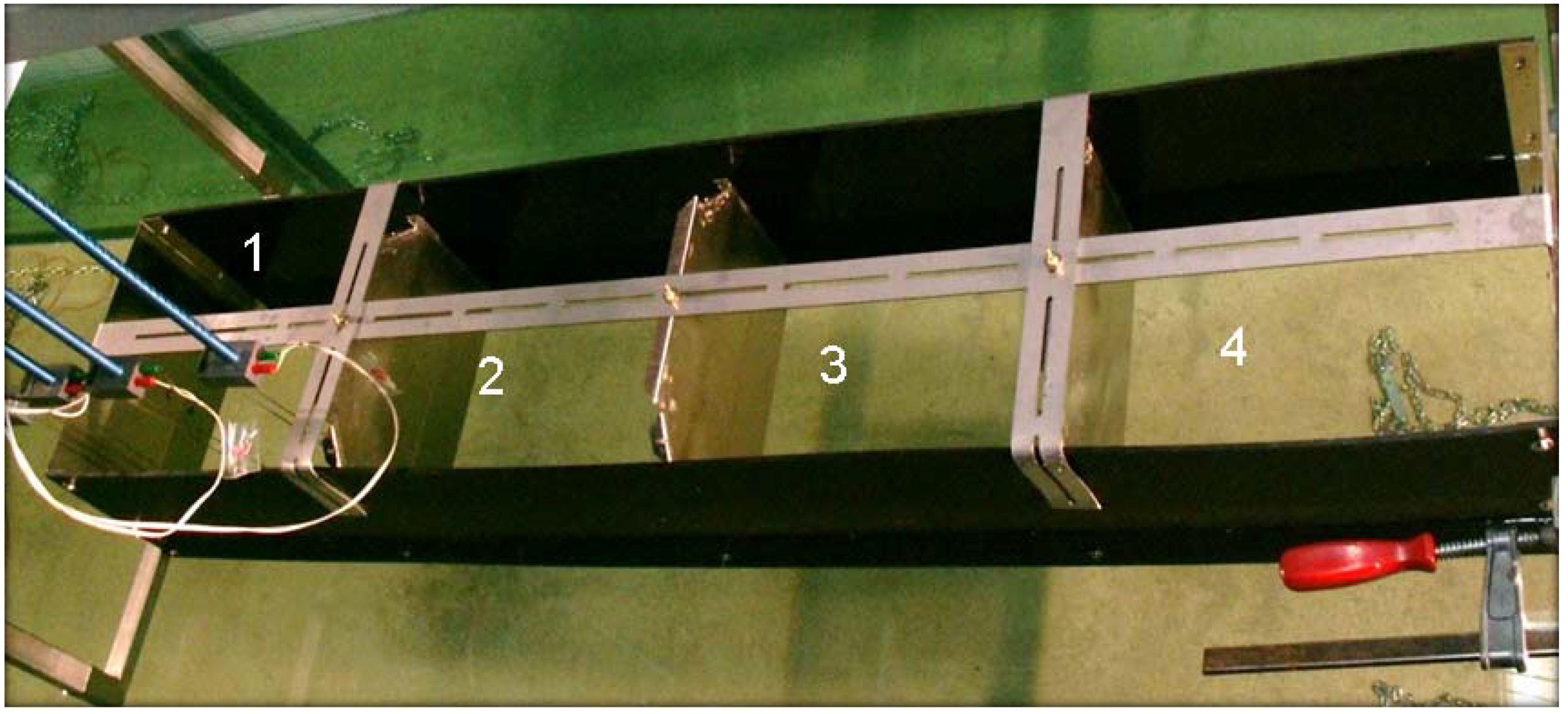
4. Physical Model Tests
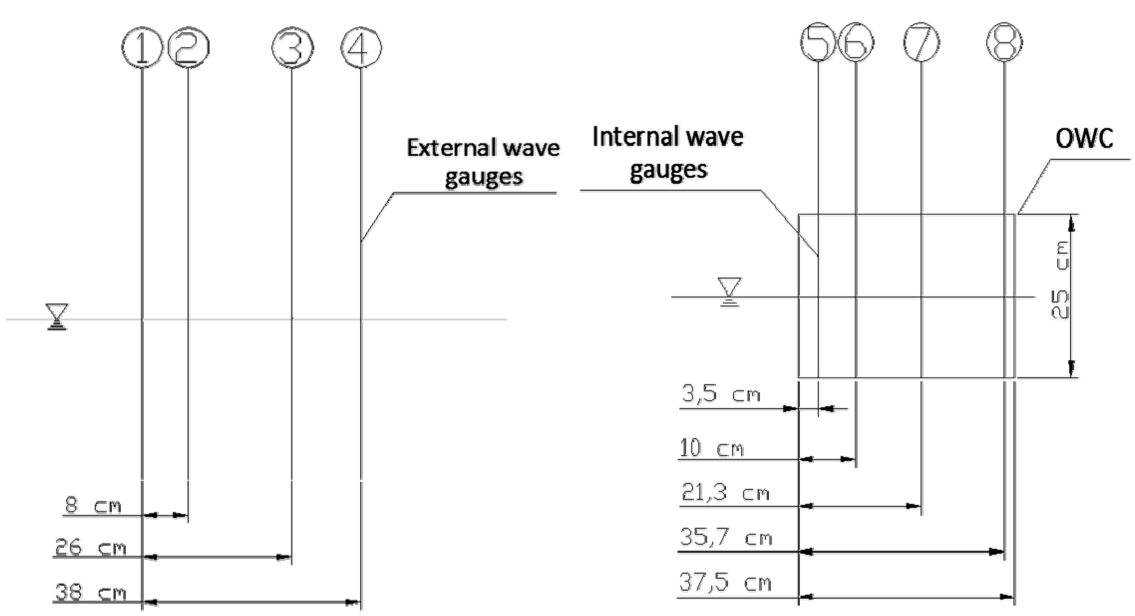
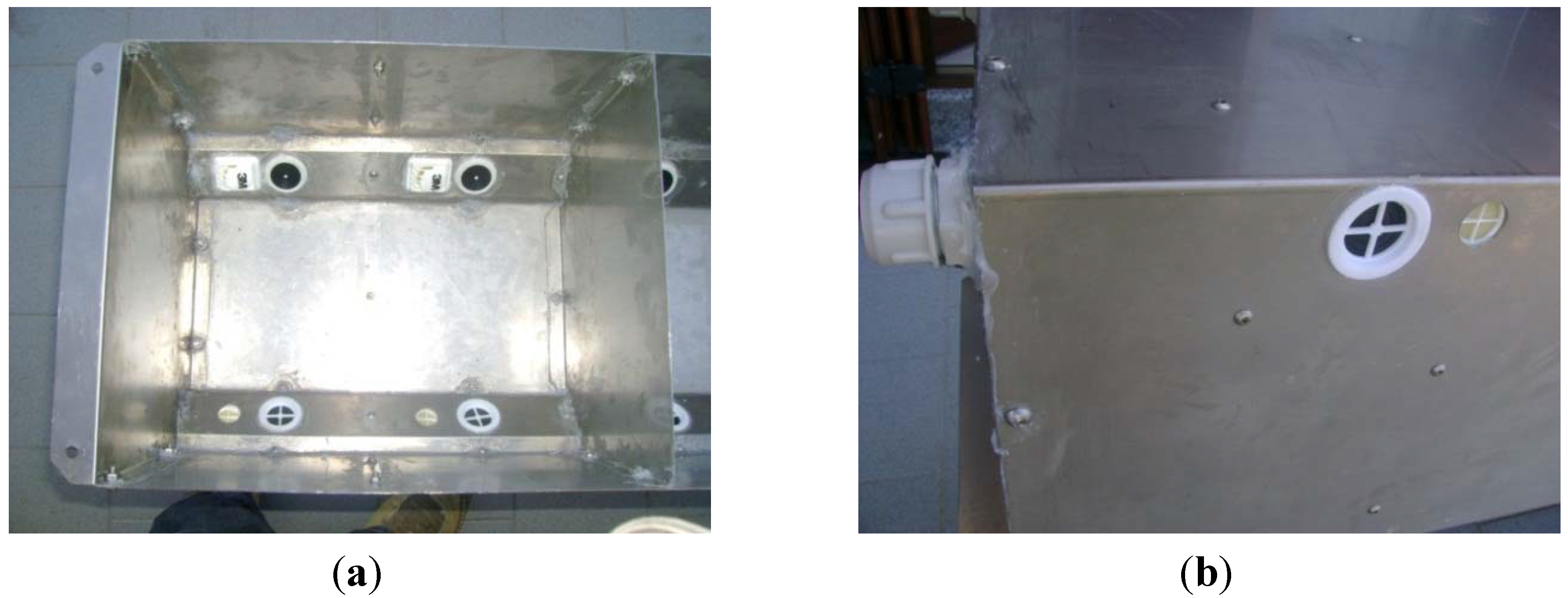
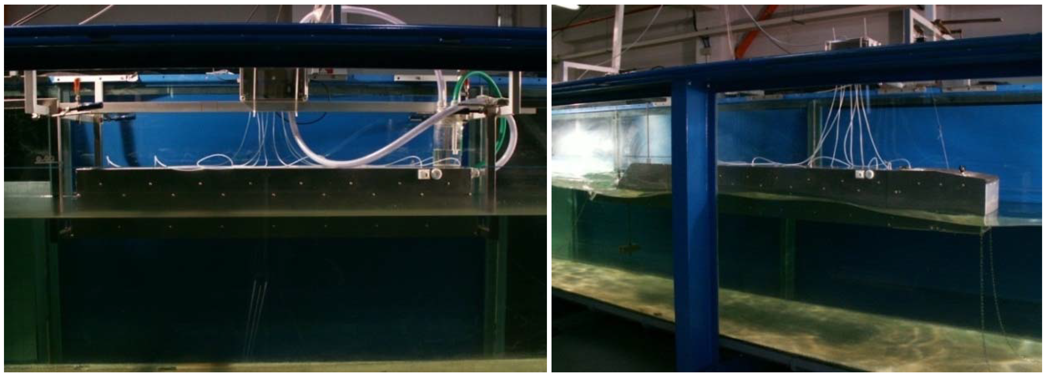
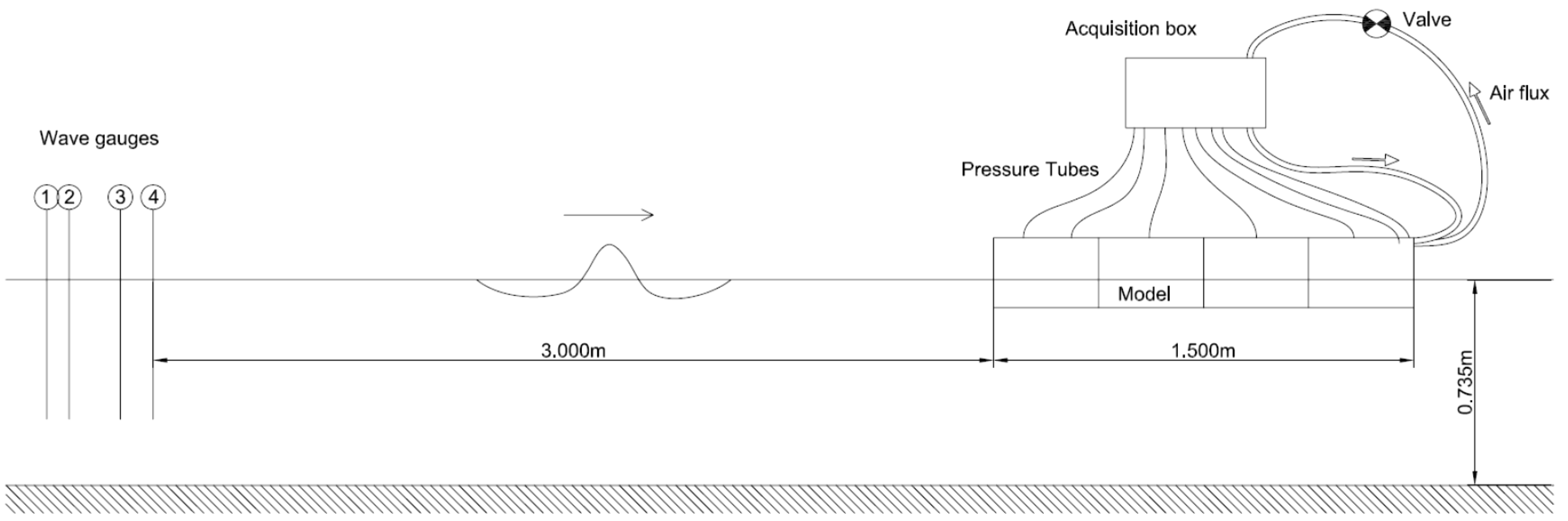
4.1. The Facility

Physical model tests on the SeaBreath were carried out in the 36 m × 1.0 m × 1.4 m wave flume of Padova University described for instance in [25]. The wavemaker is an oleodynamic rototranslational paddle equipped with a hardware wave absorption system.
To perform the tests, a fixed bottom was used. Water depth at the structure was 0.735 m. In these conditions, the maximum significant wave height that can be generated is 0.25 m (for a frequency of 1.0 Hz).The available instrumentation, used in the tests, is formed by eight wave gauges, four load cells, six air pressures transducers and one flowmeter.

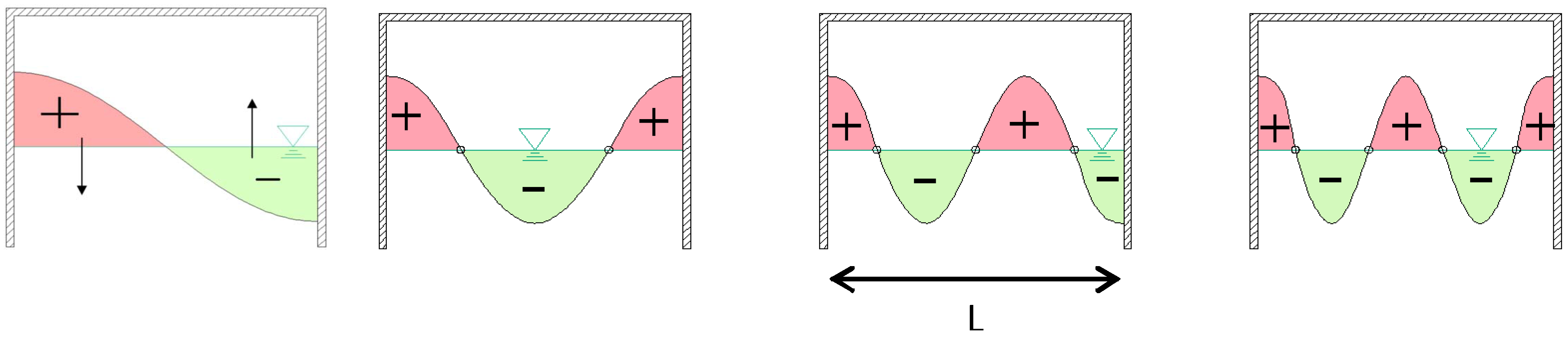
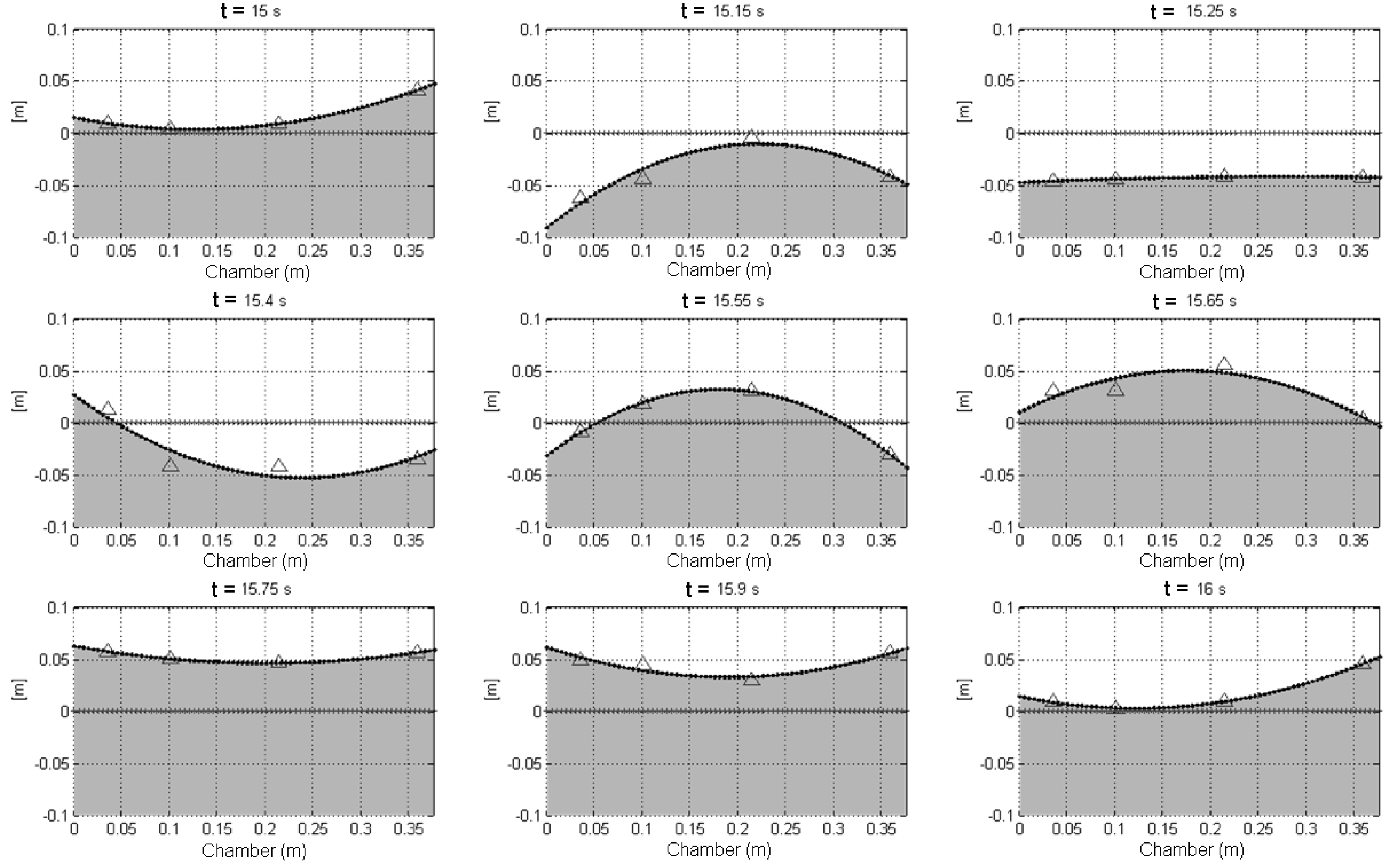
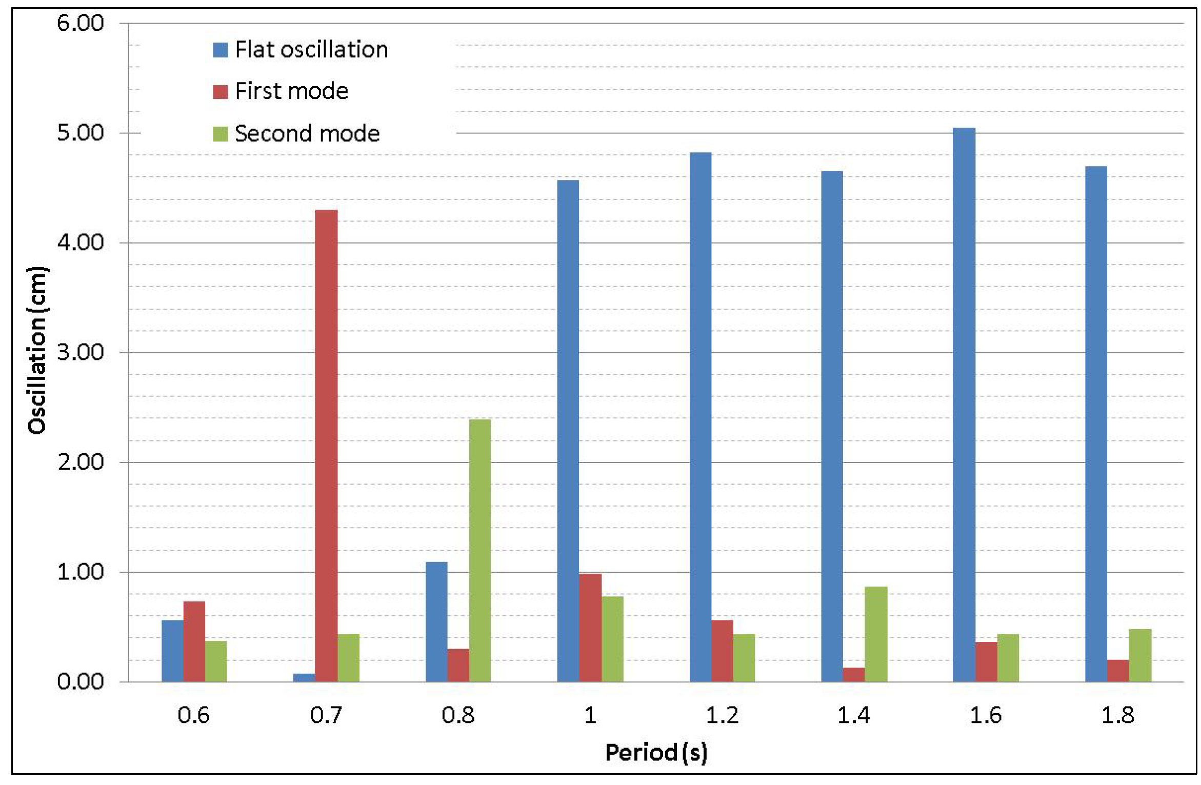
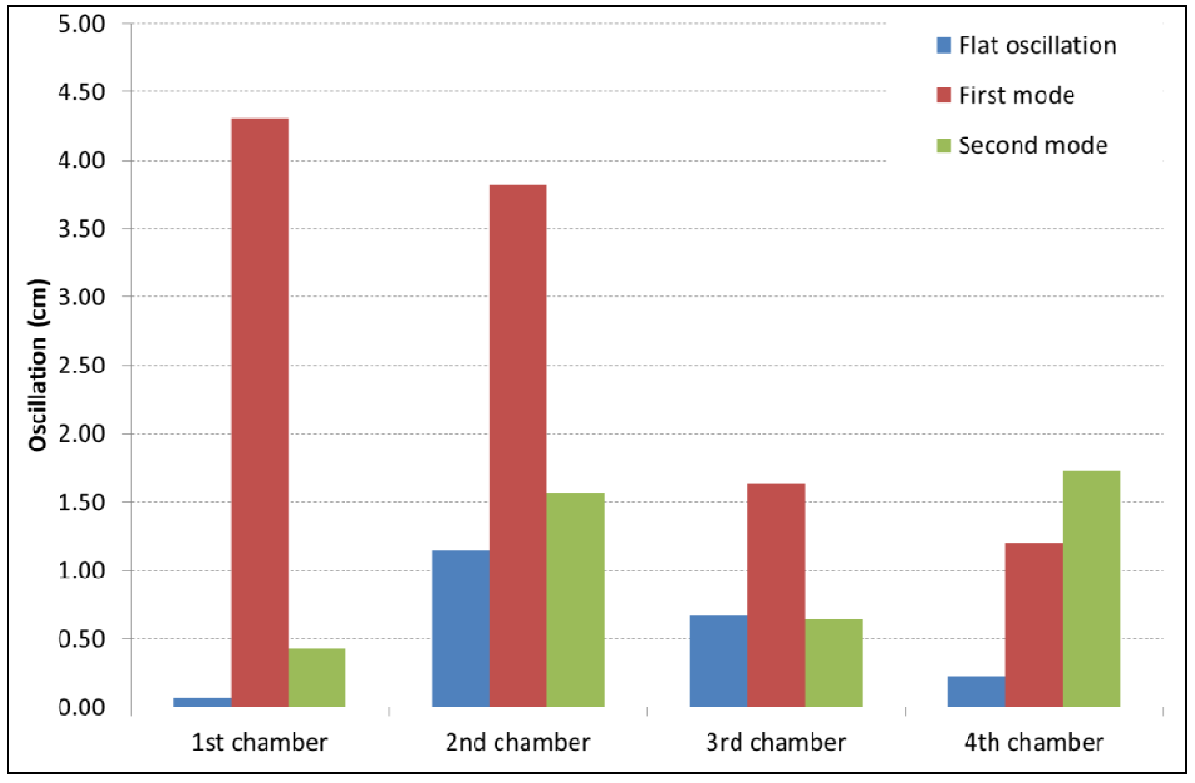
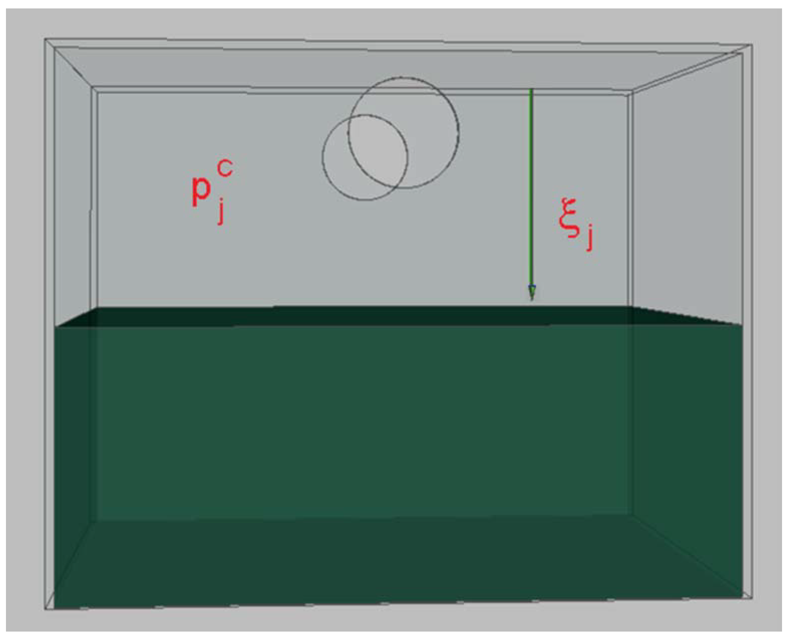
4.2. Motion of the Free Surface inside the Chambers

The first series of tests aimed at the evaluation of the free surface oscillations inside the chambers. Tests are described in detail in a MS thesis ([26], in Italian).
The first studied model is fixed, 1.5 m long, 0.3 m wide, subdivided in four chambers of equal length open both above (freeboard 12.5 cm) and below (draft 12.5 cm).
Since the wave flume is 1.0 m large, this setup corresponds to the case of an array of WECs with “permeability” of 70%.
A battery of four wave gauges (WGs) were placed 3 m in front of the device, and a second battery of four WGs were placed within each chamber. Figure 7 shows the model during setup, Figure 8 the WGs relative location.
Figure 7. The open model setup: WGs in the 1st of the four chambers.
Energies 06 04696 g007
Figure 8. Location of the WGs inside the chambers and outside the device.
Energies 06 04696 g008
The programme included 11 regular waves (H = 2 and 6 cm, T in range 0.5 s to 1.8 s) and eight irregular waves (Hs = 6 cm, Tp in range 0.6 s to 1.8 s). An exploratory investigation with different position of the internal screens was also carried out. The tests allowed a first definition of the behavior of the surface elevation inside the chambers. At the scale of the physical model investigation, air is compressed by small pressures and behaves essentially as incompressible. The numerical simulation proposed in the following takes advantage of this simplification. Prototype scale is still undefined, and may be from 10 to 100 larger than the model. Of course, in prototype air compressibility will play an important role, and will require appropriate modeling.
It was found that sloshing occur mainly in the longitudinal direction, as linear and non-linear interaction between the incident wave and the free modes. Figure 9 shows the main free modes, each of which is characterized by a single wavelength and hence a single frequency. Note that no energy is extracted in these cases, since the air volume inside the chambers does not change.
Figure 9. Free oscillations inside the chambers.
Energies 06 04696 g009
The energy is extracted only when the average water level oscillates vertically. The essence of this movement is a vertical translation of an horizontal free surface, defined “flat” oscillation hereafter.
The actual oscillations in the chambers are a sum of several modes. Nevertheless, it is assumed that the free surface can be well described considering only three degrees of freedom, i.e., the flat oscillation and the first two modes presented in Figure 9.
For each chamber, a system of equations is solved to fit the amplitude of such oscillations to the readings of the four wave gauges, with one redundant equation (four gauges and only three modes). It is easy to see that a flat oscillation induces simultaneous readings of all gauges. Similarly, other modes induce oscillations with certain fixed phase lags.
Figure 10 shows an example of the obtained fitting. Interpreted and measured oscillations of the free surface in time (t in the figure) were in good agreement, as also proved by video recordings.
Figure 10. Example of verification of the interpreted oscillations inside the chambers compared to the measurements (test with H = 6 cm; T = 1 s), for different times (t).
Energies 06 04696 g010
Figure 11 shows the height of the three modes of oscillation within the first chamber, for regular wave tests with H = 6 cm and varying period. The first mode occurs at 0.7 s, i.e., when the wavelength is twice the length of the chamber. In this case, measurements show that there is no average vertical oscillation, i.e., no energy can be extracted. Conversely, very long waves mainly cause the flat oscillation, which is suited to produce energy. Measurements also show energy transfer between frequencies, i.e., the regular incident wave is characterized by one frequency whereas the energy within the chambers is distributed also among other frequencies.
Figure 11. Height of the oscillation within the first chamber, for regular wave tests with H = 6 cm and varying period.
Energies 06 04696 g011
One of the critical issues of the model is the prediction of the wave decay along the chambers. This will be examined also in Subsection 4.3. Figure 12 shows an example of this analysis, and particularly the interpreted height of the oscillation within the four chambers, starting from the wavemaker side, for the regular wave test with H = 6 cm and T = 0.7 s, i.e., the period inducing the first free oscillation. This is the critical condition, and it can be seen that the rear chambers present a larger amplitude of the flat oscillation compared to the front one (the first). Comments on higher order power extraction modes, e.g., second order piston mode, may be found in [26].
Figure 12. Height of the oscillation within the four chambers, for a regular wave test with H = 6 cm and T = 0.7 s (i.e., the period inducing the 1st mode oscillation).
Energies 06 04696 g012
In conclusion, the analysis of all tests allowed the definition of an experimental relation between the incident wave height and the oscillation within each chamber (that, in case of linear theory, can be easily found [27]). In [28] an analytical approach is used to find the sloshing modes, even in the transverse direction.

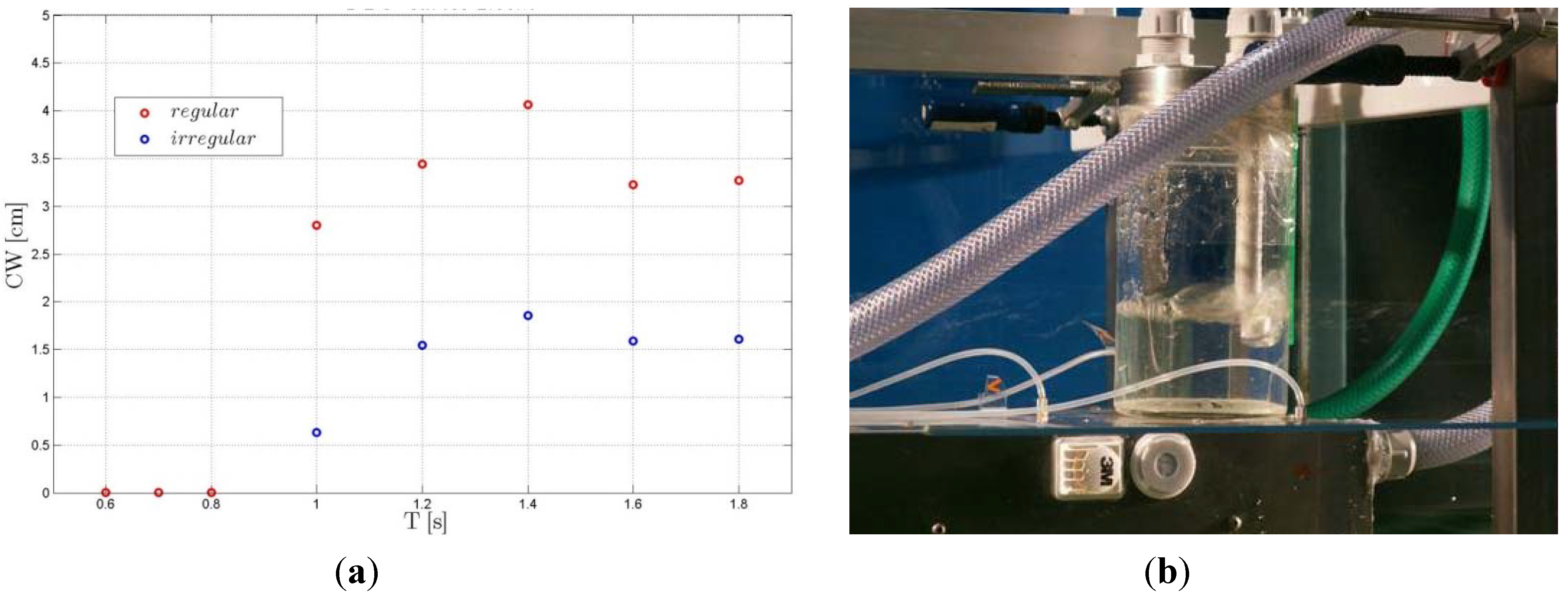
4.3. The Closed Model

A second series of tests was carried out using a structure closed above, where also the power take off (PTO) system was modeled. The head loss induced by the turbine is ideally the sum of a constant term and a term proportional to the kinetic head. The power take off was simulated in two ways: in the first case, the proportionality term is varied using a faucet mounted between the high and low pressure ducts; in the second case, the constant term was varied by forcing the air to flow inside a glass bottle with controlled water level.
Both fixed and floating configurations were analyzed, recording the air pressure both in the chambers and in the air ducts. In some cases, also the induced air flowing through the PTO was measured.
Figure 13 shows the fixed (left) and the chain moored floating (right) structure in the flume. Figure 14 shows a sketch of the setup including the measuring system. Figure 15 shows a detail of the used non-return valves. Unfortunately, the valves were seen to be very small, causing large dissipations. The prototype is now designed to have much larger valves, i.e., a continuous line of clapet valves.
Figure 13. The closed model setup in fixed and floating configuration.
Energies 06 04696 g013
Figure 14. The closed model setup with measuring system.
Energies 06 04696 g014
Figure 15. (a) Detail of the valves connecting each chamber to the low and high pressure ducts; and to (b) the external environment.
Energies 06 04696 g015
The test program includes the same wave attacks already tested for the open structure: 11 regular waves, with varying load (degree of aperture of the faucet) in the PTO, aiming at the definition of the optimal load for each wave; eight irregular waves with the load defined on the basis of the regular ones, aiming at an evaluation of the device efficiency.
Figure 16 shows an example of the obtained results in terms of capture width, as a function of the period, for regular and irregular waves. The capture width appears to be very low: much better behaviour is expected for larger valves, as shown in the following Section (Section 5.4).
Figure 16. (a) Capture width for regular and irregular wave attacks, with the load loss induced by the system shown on the right; (b) glass bottle with pipe submerged 1.5 cm, through which air is flowing.
Energies 06 04696 g016
The tests show that, even for long waves, the device efficiency is similar to the maximum. On the contrary, other M-OWC devices show a marked reduction of the efficiency for long waves, due to the absence of a communication between the chambers and the external atmosphere.
Figure 16 also shows that under irregular waves, the obtained efficiency is lower than under regular waves, confirming the importance of testing the device under wave attacks as real as possible.
When floating, the device showed a maximum efficiency for a peak wavelength equal to the structure length. In fact, for very long waves, the device “rides” the waves, with lower water oscillations in the chambers.

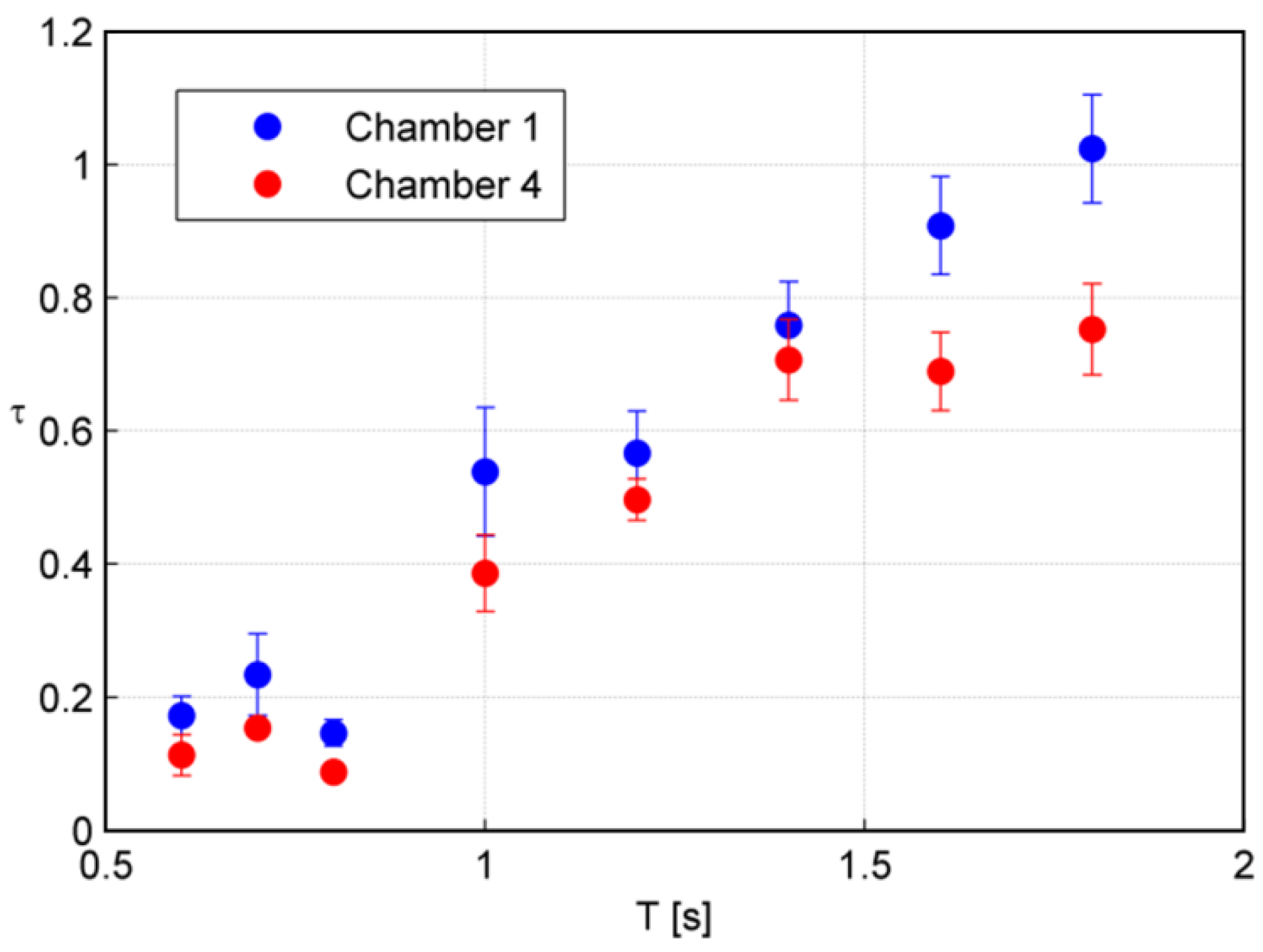
4.4. Chamber Transfer Function

A monochromatic wave induces pressure oscillations inside each chamber, with the same frequency ( ω ), but different amplitude. Let Ψ j ( ω ) be the height (double amplitude) of j-th chamber pressure fluctuation within a wave period; and H i n c ( ω ) the incident wave height.
These two quantities are related by a linear transfer function τ j ( ω ) according to:
Ψ j ( ω ) = γ w τ j ( ω )   H i n c ( ω )
The linearity of the process has been confirmed by the experiments. For incident waves of same frequency and different height, τ j ( ω ) remained almost constant. Figure 17 shows an example of chamber transfer function vs. the incident wave period ( T = 2 π / ω ), with the observed variability. Two transfer functions are plotted, relative to the front (n° 1) and rear (n° 4) chambers. As expected, the oscillation in the rear chamber are smaller than in the front one. Note that the energy may also flow inside the chambers from the sides of the device (the flume lateral walls are 35 cm apart).
Figure 17. Transfer functions for the front and rear chambers. Error bars account for standard deviations of the data set.
Energies 06 04696 g017

5. Numerical Model

This section provides the description of a simple lumped model for the analysis of power production sensitivity to the number of chambers of the Seabreath and the dimensions of the air ducts.

5.1. Air Circuit

The model simulates the flow inside the pipes of the Seabreath. Hydrodynamic coupling in the system of multiple M-OWC has been considered by using experimental transfer functions between water level in front and inside the four chambers (Section 4.3).The equations governing the flow between the chambers and the ducts (through the non-return valves) are described in Sub-section 5.2.
For the simulation of the air circuit, the dependent variables are the flow discharge (Q) in the high and low pressure circuit along the branches, represented by green arrows in Figure 18, and the pressures p* and p at the upstream and downstream nodes of the branches.
Figure 18. Reference sketch for Seabreath air circulation model.
Energies 06 04696 g018
For the evaluation of the pressure along the duct, at the intersection with the valves, two approaches are used: along the high pressure ducts, i.e., in case of inlet valves, the moment equilibrium is used (no need to evaluate the losses), whereas along the low pressure ducts (outlet valves) it is convenient to use energy balance (i.e., no losses). Figure 18 and Figure 19 show the node numbering convention and a sketch of variation in the total head along the high pressure duct. Flow along branch j − 1 and j assume the subscript of the upstream node (j − 1).
Figure 19. Energy or pressure behavior along the high pressure duct.
Energies 06 04696 g019
Mass conservation is imposed assuming air as an incompressible fluid (suitable for the interpretation of small scale tests). Mass balance requires that the flow in the downstream pipes is equal to the upstream one plus the discharge through the valves:
Q H j = Q H j 1 + Q j I     j = 1 , N
where Q j H is the air discharge in the j-th branch of the high pressure duct; Q j I is the inflow discharge through the j-th valve.
Assumed a uniformly distributed flow across the pipe, the momentum balance along the high pressure duct is:
p j * Ω + ρ a Q H j 1 2 Ω = p j H Ω + ρ a Q H j 2 Ω   j = 1 , N
where, pH is air pressure and Ω is the pipe cross section; ρ a is air density.
According to Equation (3), the pressure head and the total head decrease as the air flows past the valves. In fact, the air discharge arriving from branch j − 1 needs to accelerate the inlet valve discharge and redirect it along branch j. In detail, it is found that:
p j H ρ a g p j * ρ a g = 1 g Ω 2 ( Q H j 2 Q H j 1 2 )     j = 1 , N
( p j H ρ a g + Q H j 2 2 g Ω 2 ) ( p j * ρ a g + Q H j 1 2 2 g Ω 2 ) = 1 2 g Ω 2 ( Q H j 2 Q H j 1 2 )     j = 1 , N
where the Equations (4) and (5) give, respectively, the pressure head loss and the total head loss across the valves (see also Figure 19). Note that the term in parenthesis in the right hand side of Equations (4) and (5) are always positive.
Along the branch of the pipe, the energy decreases due a distributed loss. For a pipe of constant section, the loss along branch j − 1 is:
( p j 1 H ρ a g p j * ρ a g ) = λ L 2 g D h , i Q H j 1 2 Ω 2     j = 1 , N
In conclusion, combining Equations (4) and (6) the relation between the pressures measured at the initial nodes of the branches (j-th and j + 1), is found to be:
( p j H ρ a g p j 1 H ρ a g ) = λ L j 1 2 g D Q H j 1 2 Ω 2 Q H j 2 Q H j 1 2 Ω 2 g     j = 1 , N
Where λ is the Darcy-Weisbach resistance coefficient; L j and D are the length and diameter of the j-th branch of the duct. It may be immediately seen that the first term on the left hand side accounts for distributed energy loss and the second term accounts for energy loss across the valve, in the tube flow direction. Equation (7) is a relation between discharge and pressure at the nodes of the high pressure duct.
For the low pressure duct, where the valves cause an outlet flow, the situation is not symmetrical. Rather than momentum balance, energy conservation is used. It is easy to see that, in analogy to Equation (7), the pressures measured at the end of j-th and j + 1st branch, are related by:
( p j L ρ a g p j 1 L ρ a g ) = λ L j 1 2 g D Q L j 2 Ω 2     j = 1 , N
The mass balance is:
Q L j 1 = Q L j Q j O     j = 1 , N
where Q j L is the air discharge in the j-th branch of the low pressure duct; Q j O is the outflow discharge through the j-th valve.
The power take off is simulated by a head loss ΔM which needs therefore to be optimized. In fact, if ΔM is set to zero, the flow through the turbine will be maximum, but no energy will be produced. Similarly, if ΔM is too high, no flow will circulate. An intermediate head loss will give the maximum output. The head loss between the nodes placed upstream and downstream the turbine (Figure 18) is:
( p N + 1 H ρ a g p N + 1 L ρ a g ) = Δ M + λ L T D ( Q N H + Q A ) 2 Ω 2
where QA is the discharge that may enter from the valve that opens the circuit to the atmosphere, LT the length of the circuit connecting the high and low pressure ducts to the turbine. The flow through the turbine is defined as Q T = ( Q N H + Q A ) . Since there is some energy loss along this circuit, there is always a small difference between γwΔM and the pressure between the two pipes. Therefore the experimental values, which do not account for this loss, is slightly overestimated.

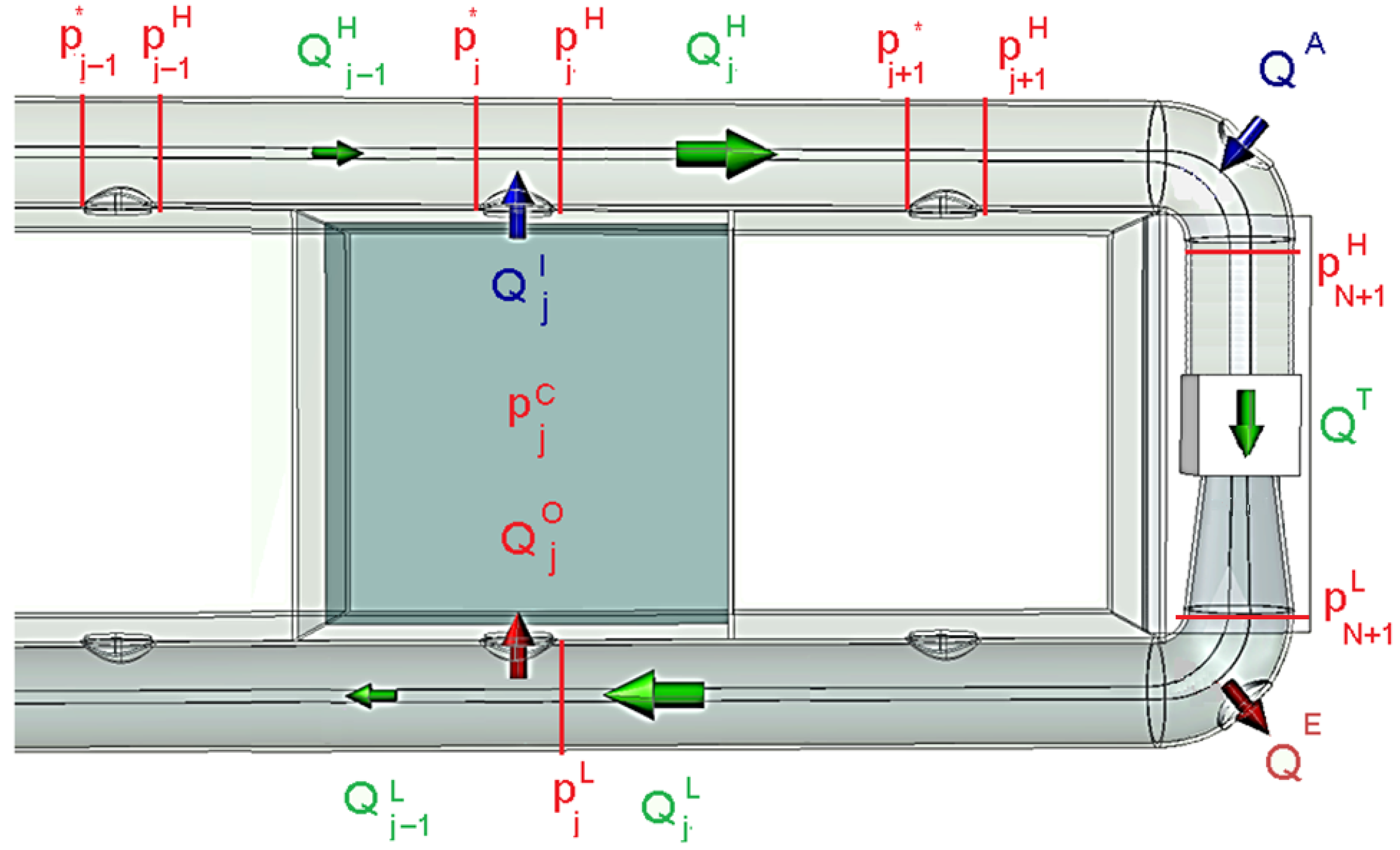
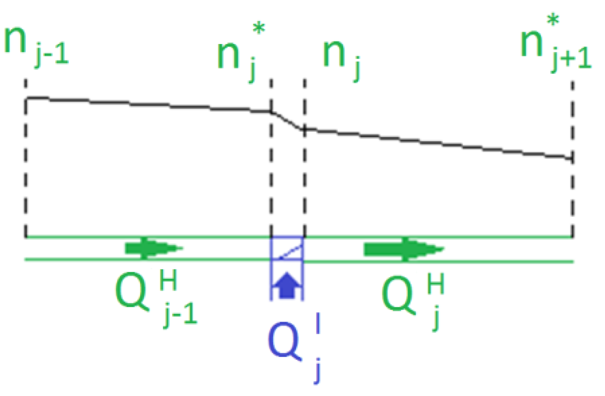
5.2. Flow between Chambers and Main Ducts

With reference to Figure 20, the air volume V in the chamber is defined as:
V j = A ξ j
where ξj is surface elevation and A is the area in the j-th chamber. Note that the maximum oscillation is obviously limited by the height of the chambers.
Each chamber is treated as a reservoir:
Q j O Q j I = V j t
The mean water level oscillation or the pressure within the chamber are given by:
ξ j = τ 0 , j ( ω ) η i n c i f p j C = p a t m p j C = γ w τ 1 , j ( ω ) η i n c i f   Q j O = Q j I = 0
where patm is the atmospheric air pressure; τ o , i ( ω ) and τ 1 , i ( ω ) are the experimentally based transfer function from wave height to chamber head for the two extreme cases of chambers open above or completely sealed.
It was found (experimentally) that:
τ 0 , j ( ω ) τ 1 , j ( ω )
Hence the average transfer function τ is defined and, in the general case, the total head inside the chamber is given by the sum of elevation and pressure head (neglecting the kinetic head), i.e.:
τ j η i n c = ξ j + p j C γ w
The chamber volume (8) is thus approximated as follows:
V j = A ( τ j η i n c p j C γ w )
Figure 20. Reference sketch for model chamber.
Energies 06 04696 g020
Finally, chamber orifices are modeled by monotonic discharge laws. Assuming a threshold resistance for valve opening ( ε ):
Q j I = c q a 2 ρ a ( p j C p j H ε ) Q j O = c q a 2 ρ a ( p j L p j C ε )   j = 1 , N   (or zero if complex)
where cq is a discharge coefficient; and a is the valve aperture area.
Similarly, the discharge entering form the valves open to the atmosphere are:
Q A = c q a 2 ρ a ( p a t m p N H ε ) Q j E = c q a 2 ρ a ( p N L p a t m ε )   (or zero if complex)
The discharge in Equation (18) depends on a value of pressure that is not exactly coincident with p N H or p N L ; but the expected error of Equation (18) is small. In practice, the discharge may be evaluated based on p N + 1 H or p N + 1 L if more convenient.
By substituting the discharge in each chamber, Equation (12) becomes:
1 γ w p j C t = τ i η i n c t + c q a A 2 ρ a ( p j L p j C ε   p j C p j H ε )     j = 1 , N
Equation (19) gives a system of ordinary differential equations, solved in time.

5.3. Solution Procedure

The so called methods of nodes is used to solve the circuit in Section 5.1 (i.e., the discharges are expressed in terms of pressures, and the continuity equation appear as balances between pressures) and Equation (19) is used to evolve the pressure in time. The discharge along the circuit Q = [ Q 1 H ,   , ] (including the discharge along the turbine QT) is expressed according to of Equations (2) and (9) in terms of discharge across the valves q = [QI, QO, QA, QE]. A matrix is set up, that for the case of two chambers, reads:
[ Q 1 H Q 2 H Q   T Q 2 L Q 1 L 0 ] = [ 1 0 1 1 0 0 0 0 0 0 0 0 1 1 1 1 1 0 1 1 0 0 0 0 1 1 1 1 1 1 1 1 1 0 1 1 ]   *     [ Q 1 I Q 2 I Q   A Q   E Q 2 O Q 1 O ]   i = 1 , N
where the last line is not used to derive the discharge, and it is shown here only to point out that there is a condition among the discharges through the valves q that must be satisfied.
The choice of the load on the turbine Δ M is defined a priori. The unknowns are the pressures along the circuit P, and the pressures in the chambers p. For the two chamber case is P = [ p N H ,   p 2 H ,   p 3 H ,   p 1 L ,   p 2 L ,   p 3 L ] , and p = [ p 1 C ,   p 2 C ] .
For each new instant, p is derived from Equation (19), based on old values. It is easy to see that the (tentative) knowledge of P would allow to define directly q, i.e., the discharge entering or leaving the duct from the chambers, thanks to Equation (17), and from the atmosphere, thanks to Equation (18). The set of Equations (20), except the last one, are used to write a relation between q and Q. It is then possible to verify if the tentative values in vector Pare consistent: Based on Q, the different values of P are related by Equation (7) for the HP circuit, by Equation (8) for the LP circuit and by Equation (10) for the flow along the turbine. Further, the last line in Equation 20 should also provide the overall continuity requirement.
Note that most of these equations are non-linear and several false solutions may appear if the tentative values of P are not constrained. Therefore the following procedure was adopted, that is based on a physical understanding of the process. The pressures p in the chambers at time t + dt are found for every time step based on Equation (19) and the initial condition is the atmospheric pressure at all nodes. Then, in chamber 1 the high pressure p 1 H is varied from 0 to the pressure in the chamber p 1 C , and the remaining pressures P are evaluated in cascade from upstream. If a value of pressure (in this range) is found to satisfy the continuity equation, such value it is considered valid. Else, it means that no flow exits from chamber 1, p 1 H is not computed ( Q j I = 0 and there is no more interest for p 1 H ) and the pressure p 2 H is searched for. The procedure follows for all the values of p j H . If no solution occurs for any of p j H , it means that no air is flowing from the chambers to the high pressure duct (but it may enter from the atmosphere). In this case, the procedure then tries to vary the pressure p 1 L between 0 and the (negative) pressure in the chamber p 1 C . If no solution is found, p 1 L is not computed (also Q j O = 0 and there is no more interest in p 1 L either) and so on. In case no solution is found, it means that no air is flowing at all (static conditions), as it is impossible that the flow is driven only by the atmosphere.
Note that if ξ exceeds the chamber dimensions, ξ is limited and the pressure in the chamber is fixed.

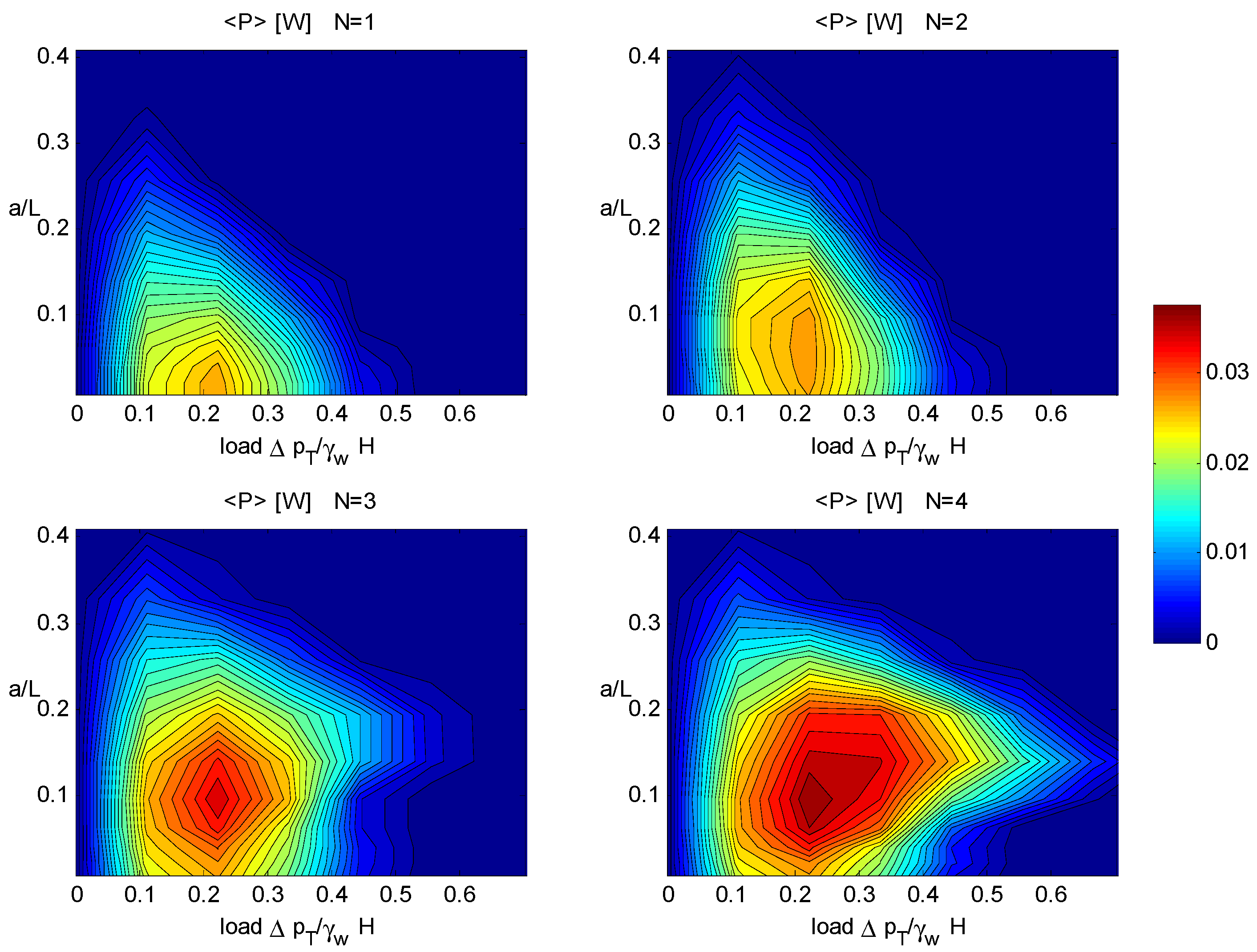
5.4. Interpretation of Experimental Results

In order to check the model capabilities, the small scale tests have been numerically simulated. The numerical and experimental results relative to the power production for different wave periods (but same H), loads in the PTO, number of chambers and chamber length to wavelength ratio (a/L) were compared. The machine average power production, within one wave period T, are experimentally evaluated as:
P = 0 T Δ p T Q d t
where Δ p T is the measured pressure difference between the high and low pressure ducts. The comparison between numerical and experimental model results is satisfactory. For instance, for a capture width in Figure 16 equal to 0.03 m, H = 0.06 m, T = 1.0 s, the associated total power is:
P = E C g C W = 0.044   W
A small difference between the results in Figure 21 and Figure 22 and the above value is due to the difference between Δ p T in Equation (21) and γw Δ M (the actual head loss before and after the PTO, used to define the numerical power).
Figure 21. Average power production for regular waves considering up to N = 4 chambers.
Energies 06 04696 g021
Figure 22. CW as function of the valves diameter.
Energies 06 04696 g022
Figure 21 shows contour graphs for Equation (21) adopting the geometry used in the experiments, i.e., chamber length “a” is 25 cm, tubes and valves diameter is 2 cm and wave height 10 cm. Average power is plotted against non-dimensional wave length (ordinate) and net loss (abscissa), for different numbers of chambers.
It is seen that, for a single fixed chamber OWC (length equal to “a”) the most effective wave length is infinitely long (best a/l = 0 for N = 1). With increasing number of chambers, the optimum wavelength decreases to some finite value (e.g., for a wave 100 m long, the device should be formed by four chambers, each 10 m long). The figure also defines the optimum load on the PTO ( Δ p T ).

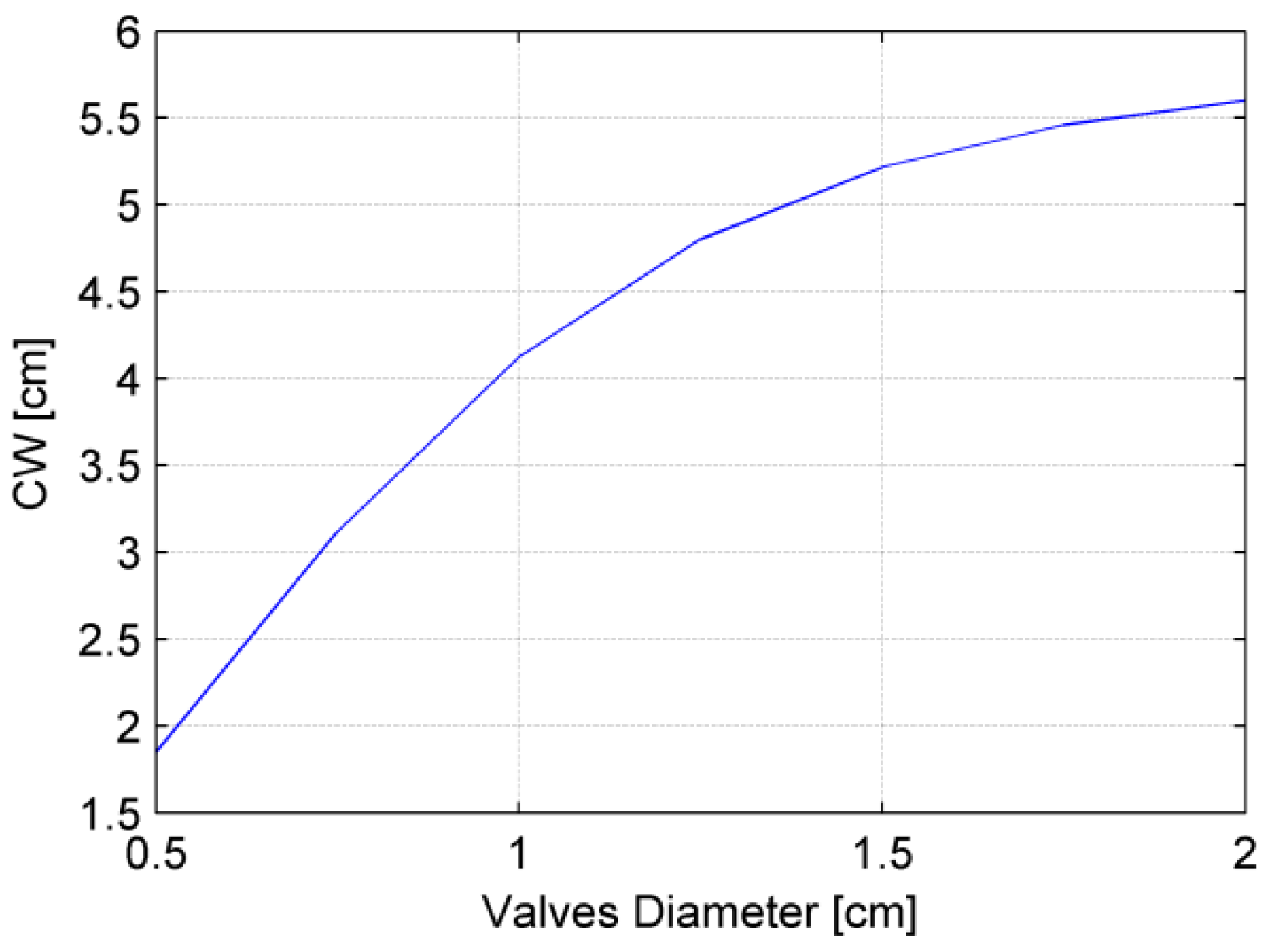
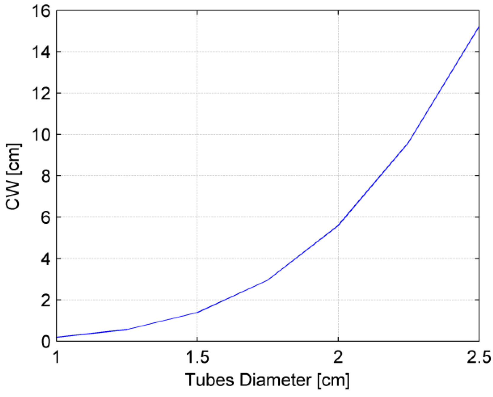
5.5. Capture Width for Improved SeaBreath
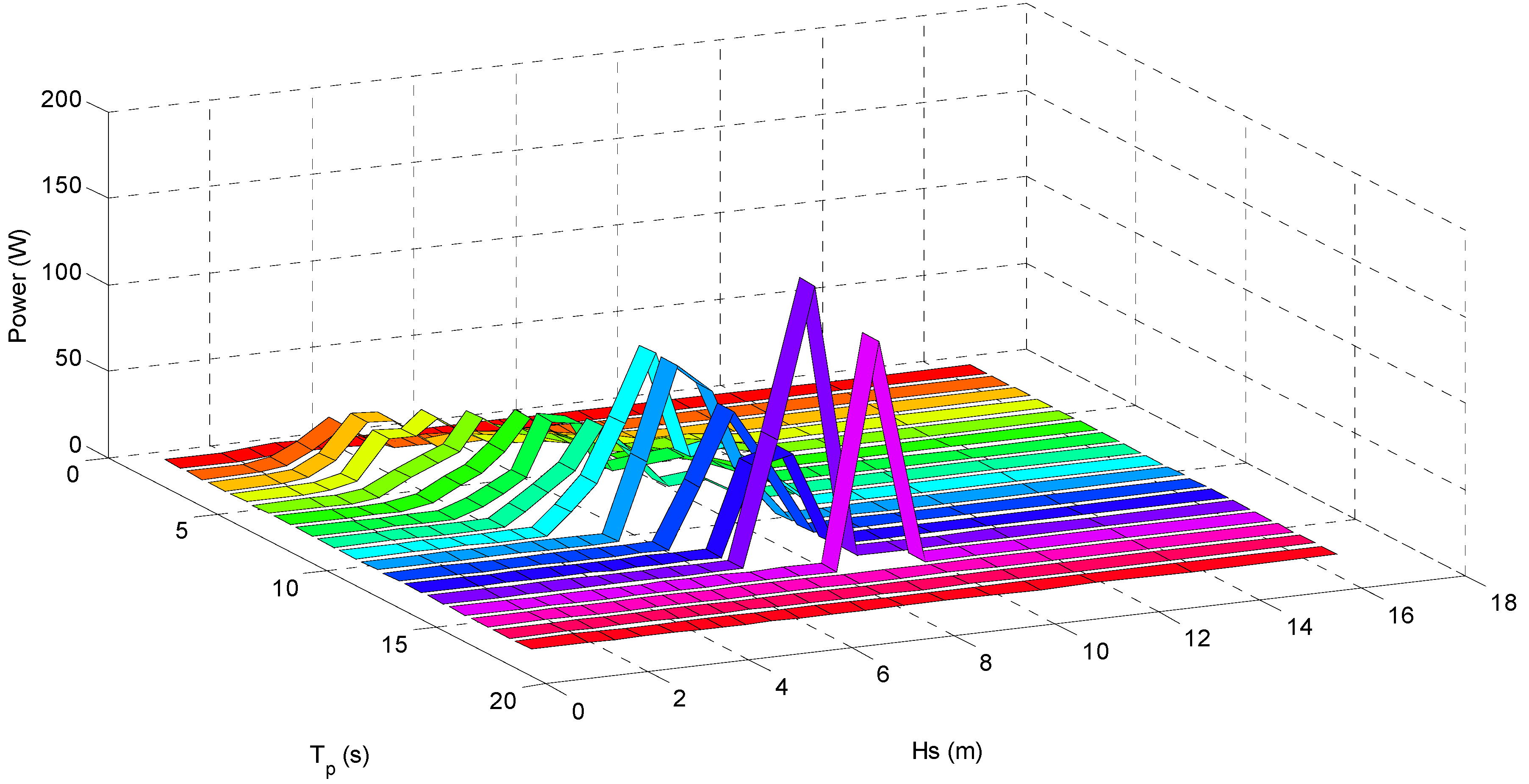
By fixing the optimum machine head loss at Δ M = 0.2   γ w H i n c , the system of equations described above can be used to study the sensitivity of the system with respect to valves and tubes diameters.
First, the tube diameter was assumed to be 2 cm, and valves are varied in the range 0.5–2 cm. Chamber length is 25 cm. Figure 22 is obtained for waves of height 6 cm and period 1.4 s. As expected, the resistance of the valves plays a fundamental role on the capture width (i.e., device efficiency).
In a second analysis, the tube diameters is varied from 1 to 2.5 cm, and the valves are constrained to have the same area of the pipes (all other variables are fixed). Results are given in Figure 23.
It is seen that for a slight increase of the ducts (from 2 to 2.5 cm) resonant conditions are almost reached and the capture width is more than doubled. For this case, the maximum volume in the chambers is reached.
Figure 23. CW increase with tubes diameter up to resonant conditions (valve and pipe diameter are equal).
Energies 06 04696 g023

6. Application

In view of a possible experimental application in the field, a location in the Southern part of Emilia Romagna Region (e.g., Riccione), is tentatively selected. The expected wave climate is given in Figure 24, representative of the reach n. 3 (see Figure 4). Total energy is 2.5 kW average.
Figure 24. Average wave energy flux for different classes of Tmo and Hs.
Energies 06 04696 g024
In several beaches of the Southern coast of Emilia Romagna, low impact innovative solutions have been tested [29] as alternative to traditional barriers or groynes for coastal protection, gaining the approval of stakeholders. The expected reduction of the waves incident the coastline would very likely be welcome and it could build up to the effect of the existing submerged sand bag barriers. Furthermore, a directional wave buoy is operating, and could monitor the incident waves for monitoring purposes.
In order to understand the actual potential, the model described above was used, for a prototype 30 m long, 6 m wide, 5 m high (20 times larger than model tested in the flume, 5 times smaller than a prototype considered to be “economically viable”), moored and weathervaning in order to have the axis parallel to the incident wave direction. The assumed diameter of the ducts is 0.5 m (after the 1:20 upscaling). Table 1 summarizes the results obtained multiplying the available energy in the site, subdivided in class of equal peak wave period (Tmo), by the Seabreath capture width (CW) relative to each Tmo. It may be observed that the device could generate 6605 W, with an overall capture with of 6.6 kW ÷ 2.5 kW/m ≅ 2.6 m .Since the designed Seabreath width is 6 m, it is found that the (quarter scale) device extracts 43% of the energy incident the front. Further optimization of the geometry is ongoing.
Table 1. Energy produced by a 6 m wide Seabreath, subject to a mild wave climate of 2.5 kW/m. The device efficiency (or capture width) is best for periods close to 6 s.
Wavegruop (n°)Tmo (s)Power (W/m)CW (m)Producedenergy (W)
1calmsea00.00
21.9610.10
32.4860.10
43.00270.12
53.63940.214
64.171011.1106
74.591202.3271
85.051592.4382
95.552202.6576
106.113053.0915
116.723802.91111
127.394382.91248
138.134592.91309
148.942242.9637
159.84122.933
1610.8302.90
Total:6605
The energy extracted according to Table 1 accounts also for the contribution of the maximum wave, with power 400 kW. Economic considerations suggest that the turbine is designed for a much lower value, and protected against overloads, although the energy of the higher waves will not be completely converted.
For this early stage of design, in [30] a method is suggested for a reasonable choice of the PTO design power at full scale, accounting for economic considerations. However, for quarter scale applications, the main benefit of the research project is the demonstration of the technology, regardless of the actual amount of produced power. Accordingly, a very low-cost (off the shelf) 3 kWp turbine is considered in the design. For this case, a simple analysis was carried out, based on the table of available power per unit width, defined for several classes of Hs and Tp (see Section 2). The power per unit width is multiplied by the corresponding CW. Using the hypothesis 1 in [29] (i.e., when the available power exceeds 3 kW, the turbine is operated at this rate, and part of the flow is diverted to the atmosphere), the device can convert 1340 W in average (yearly production of 11.7 MhW/year), corresponding to a capacity factor of 0.4 (i.e., as if the turbine produced energy for 40% of the time).

7. Conclusions

This note presents a map of the wave energy in the Mediterranean Sea and introduces a new WEC device named Seabreath. Physical model tests were carried out on two types of models. The first one was open above and below and fixed to the bottom. The second model was closed above, thus creating oscillating water chambers as in the real device. For the latter case, both fixed and floating configurations were tested. The tests allowed a clear characterization of the movements of the surface elevation in the chambers and of the flow in the ducts. Unfortunately, the model dimensions were far from ideal and in particular the valves and the ducts were too small to allow an efficient air flow. As a consequence, the measured efficiency was low. A simple model has therefore been setup that derives a relation between incident waves and water levels in the chambers from the experimental model, and simulates the air flow. The model is able to reproduce the experiments. Based on the model predictions, a suitable design is proposed, with ducts 2.5 times larger and valves open along the whole chamber length. The obtained efficiency is then used to simulate the possible production of the device off-shore Riccione. It was found that the device can be expected to convert 6.6 kW in average, i.e., 58 MWh/year.
This quarter scale installation should be considered as an essential stage to proceed in the R&D of the device. Obviously, for full scale installations, costs and energy production scale differently. For example, since the energy production increases proportionally to the length scale raised to the power 3.5, for a prototype four times larger (120 m long, 24 m wide, 20 m high), located in a correspondingly more energetic sea (i.e., Portugal), the expected potential production would be 850 kW in average.

Notation:

a
Chamber length
D
Diameter of the duct
H i n c ( ω )
Incident wave height
j
Index for chambers (1 is closest to incident waves, N the closest to the turbine)
L j
Length of the j-th branch of the duct
LT
Length of the circuit connecting the high and low pressure ducts to the turbine
Q j H
Air discharge in the j-th branch of the high pressure duct
Q j I
Inflow air discharge through j-th valve
Q j L
Air discharge in the j-th branch of the low pressure duct
Q j O
Outflow air discharge through the j-th valve
QA
Inflow air discharge through the valve that opens the circuit to the atmosphere (depending on p N + 1 H )
QE
Outflow air discharge from the valve that opens the circuit to the atmosphere (depending on p N L )
Q   T
Air discharge through the turbine
p j *
Air pressure at upstream node j, in the high pressure duct
p j H
Air pressure at downstream node j, in the high pressure duct
p j L
Air pressure at downstream node j, in the low pressure duct
p j C
Air pressure in chamber j
V
Air volume in the chambers
ΔM
Head loss (load) through the turbine
λ
Darcy–Weisbach resistance coefficient
ξ
Distance between ceiling of device and water level in the chamber
ρ a
Air density
τ j ( ω )
Linear transfer function between incident wave and height in chamber j
τ o , j ( ω )
Experimentally based transfer function from wave height to level in open chamber j
τ 1 , j ( ω )
Experimentally based transfer function from wave height to level in sealed chamber j
Ψ j ( ω )
Height (double amplitude) of i-th chamber pressure fluctuation within a wave period
Ω
Pipe cross section

Acknowledgments

The support of the EU FP7 Theseus “Innovative Technologies for Safer European Coasts in a Changing Climate”, contract ENV.2009-1, n° 244104, is gratefully acknowledged.

Conflicts of Interest

The authors declare no conflict of interest.

References

  1. Kofoed, J.P.; Frigaard, P. Development of wave energy devices: The Danish case/the dragon of nissum bredning. J. Ocean Technol. 2009, 4, 83–96. [Google Scholar]
  2. Falcão, A.F.O. Wave energy utilization: A review of the technologies. Renew. Sustain. Energy Rev. 2012, 14, 899–918. [Google Scholar] [CrossRef]
  3. Boccotti, P. Caisson breakwaters embodying an OWC with a small opening-part I: Theory. Ocean Eng. 2007, 34, 806–819. [Google Scholar] [CrossRef]
  4. Boccotti, P.; Filianoti, P.; Fiamma, V.; Arena, F. Caisson breakwaters embodying an OWC with a small opening-part II: A small-scale field experiment. Ocean Eng. 2007, 34, 820–841. [Google Scholar] [CrossRef]
  5. Arena, F.; Filianoti, P. Small-scale field experiment on a submerged breakwater for absorbing wave energy. J. Waterw. Port Coast. Ocean Eng. 2007, 133, 161–167. [Google Scholar] [CrossRef]
  6. Martinelli, L. Wave Energy Converters under Mild Wave Climates. In Proceedings of the Marine Technology Society and the Institute of Electrical and Electronics Engineers (MTS/IEEE/MTS) Oceans Conference, Kona, HI, USA, 19–22 September 2011; p. 8.
  7. Archetti, R.; Bozzi, S.; Passoni, G. Feasibility Study of a Wave Energy Farm in the Western Mediterranean Sea: Comparison among Different Technologies. In Proceedings of the 30th International Conference on Ocean, Offshore and Arctic Engineering (OMAE2011), Rotterdam, The Netherlands, 19–24 June 2011.
  8. Vicinanza, D.; Margheritini, L.; Kofoed, J.P.; Buccino, M. The SSG wave energy converter: Performance, status and recent developments. Energies 2012, 5, 193–226. [Google Scholar] [CrossRef]
  9. Zanuttigh, B.; Angelelli, E. Experimental investigation of floating wave energy converters for coastal protection purpose. Coast. Eng. 2013, 80, 148–159. [Google Scholar] [CrossRef]
  10. Vicinanza, D.; Cappietti, L.; Contestabile, P. Assessment of Wave Energy around Italy. In Proceedings of the 8th European Wave and Tidal Energy Conference Series, Uppsala, Sweden, 7–10 September 2009.
  11. Vicinanza, D.; Cappietti, L.; Ferrante, V.; Contestabile, P. Estimation of the wave energy in the Italian offshore. J. Coast. Res. 2011, 64, 613–617. [Google Scholar]
  12. Corsini, S.; Franco, L.; Inghilesi, L.; Piscopia, R. L’Atlante delle Onde nei Mari Italiani/Italian Wave Atlas; APAT e Università di Roma Tre: Roma, Italy, 2004. [Google Scholar]
  13. Filianoti, P. Wave Energy Availability in Different Areas of the World. In Proceedings of the 27th Convegno di Idraulica e Costruzioni Idrauliche, Genova, Italy, 12–15 September 2000.
  14. Piscopia, R.; Corsini, S.; Inghilesi, R.; Franco, L. Misure Strumentali di Moto Ondoso della Rete Ondametrica Nazionale: Analisi Statistica Aggiornata degli Eventi Estremi [in Italian]. In Proceedings of the 28th Convegno di Idraulica e Costruzioni Idrauliche, Potenza, Italy, 16–19 September 2002.
  15. Liberti, L.; Carillo, A.; Sannino, G. Wave energy resource assessment in the Mediterranean, Italian prospective. Renew. Energy 2013, 50, 938–949. [Google Scholar] [CrossRef]
  16. Gaillard, P.; Ravazzola, P.; Kontolios, Ch.; Arrivet, L.; Athanassoulis, G.A.; Stefanakos, Ch.N.; Gerostathis, Th.P.; Cavaleri, L.; Bertotti, L.; Sclavo, M.; et al. Wind and Wave Atlas of the Mediterranean Sea; Western European Armaments Organization (WEAO) Research Cell, Western European Union: Brussels, Belgium, 2004. [Google Scholar]
  17. Vannucchi, V.; Cappietti, L.; Falcão, A.F.O. Estimation of the Offshore Wave Energy Potential of the Mediterranean Sea and Propagation toward a Nearshore Area. In Proceedings of the 4th International Conference on Ocean Energy (ICOE), Dublin, Ireland, 17–19 October 2012; pp. 1–5.
  18. Cavaleri, L.; Bertotti, L. The improvement of modeled wind and waves fields with increasing resolution. Ocean Eng. 2006, 33, 553–565. [Google Scholar] [CrossRef]
  19. Cavaleri, L.; Sclavo, M. The calibration of wind and wave model data in the Mediterranean Sea. Coast. Eng. 2006, 53, 613–627. [Google Scholar] [CrossRef]
  20. Ruol, P.; Martinelli, L.; Iommi, R. Mappatura Dell’ Energia Ondosa in Italia ai Fini del Possibile Sfruttamento Tramite Convertitori Ancorati al Largo [in Italian]. In Proceedings of Acqua ed Energia dell’ Accademia dei Lincei, Roma, Italy, 22 March 2011; pp. 109–116.
  21. Seabreath Home Page. Available online: https://www.seabreath.it (accessed on 30 March 2013).
  22. Thorpe, T.W. The Wave Energy Programme in the UK and the European Wave Energy Network. In Proceedings of the 4th Wave Energy Conference, Aalborg, Denmark, 4–6 December 2000; pp. 19–27.
  23. Kofoed, J.P.; Frigaard, P. Hydraulic Evaluation of the LEANCON Wave Energy Converter; DCE Technical Report No. 45; Department of Civil Engineering, Aalborg University: Aalborg, Denmark, 2008. [Google Scholar]
  24. Nautilus Footage and Testing in Moreton Bay. Available online: https://www.youtube.com/watch?v=8HYUR6Jv2nw (accessed on 30 March 2013).
  25. Ruol, P.; Martinelli, L.; Pezzutto, P. Formula to predict transmission for π-type floating breakwaters. J. Waterw. Port Coast. Ocean Eng. 2013, 139, 1–8. [Google Scholar] [CrossRef]
  26. Canale, G. Ottimizzazione di un Convertitore di Energia Ondosa a Colonna d’Acqua Oscillante Tramite Sperimentazione in Laboratorio [in Italian]. Master’s Thesis, University of Padova, Padova, Italy, 2010; p. 196. [Google Scholar]
  27. Mei, C.C.; Stiassnie, M.; Yue, D.K.-P. Theory and Applications of Ocean Surface Waves; World Scientific: Singapore, 2005. [Google Scholar]
  28. Renzi, E.; Dias, F. Resonant behaviour of an oscillating energy converter in a channel. J. Fluid Mech. 2012, 701, 482–510. [Google Scholar] [CrossRef] [Green Version]
  29. Martinelli, L.; Zanuttigh, B.; de Nigris, N.; Preti, M. Sand bag barriers for coastal protection along the Emilia Romagna littoral, Northern Adriatic Sea, Italy. Geotext. Geomembr. 2011, 29, 370–380. [Google Scholar] [CrossRef]
  30. Martinelli, L.; Zanuttigh, B.; Kofoed, J.P. Selection of design power of wave energy converters based on wave basin experiments. Renew. Energy 2011, 36, 3124–3132. [Google Scholar] [CrossRef]

