Methods for Risk-Based Planning of O&M of Wind Turbines


Abstract
: In order to make wind energy more competitive, the big expenses for operation and maintenance must be reduced. Consistent decisions that minimize the expected costs can be made based on risk-based methods. Such methods have been implemented for maintenance planning for oil and gas structures, but for offshore wind turbines, the conditions are different and the methods need to be adjusted accordingly. This paper gives an overview of various approaches to solve the decision problem: methods with decision rules based on observed variables, a method with decision rules based on the probability of failure, a method based on limited memory influence diagrams and a method based on the partially observable Markov decision process. The methods with decision rules based on observed variables are easy to use, but can only take the most recent observation into account, when a decision is made. The other methods can take more information into account, and especially, the method based on the Markov decision process is very flexible and accurate. A case study shows that the Markov decision process and decision rules based on the probability of failure are equally good and give lower costs compared to decision rules based on observed variables.1. Introduction
Planning operation and maintenance (O&M) of wind turbines is an important topic, as the costs of these are large. They contribute to around 25% of the cost of energy. Parts of the costs are due to planned O&M, but around 2/3 of the direct O&M costs go to unplanned maintenance due to the failure of components [1]. For wind turbines, component failures are relatively common. Total annual failure rates between 1.5 and 4 are reported for onshore wind turbines [1]. Most failures are minor and result in relatively short downtime per failure, even though it adds up due to the many occurrences. Large failures are more rare, but they come with a long downtime and expensive repairs. Catastrophic events with total collapse of the turbine are even more rare and will come with large economic loss. However, compared to other structures, pollution and the risk of the loss of human lives are generally very small.
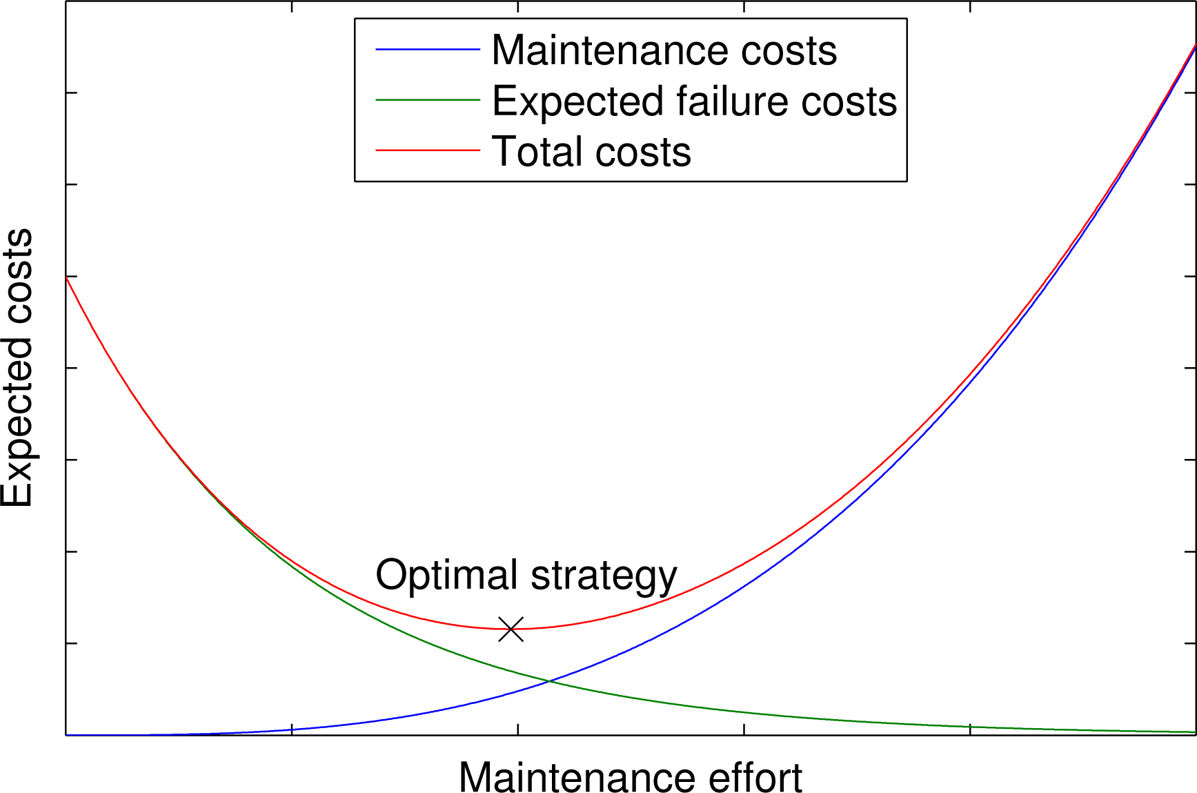
In many components, deterioration processes, such as fatigue, wear and corrosion, cause failures, for example in welded connections, blades, bearings and gears. In those cases, it could be possible to detect the damages before actual failure and, thereby, perform preventive maintenance instead of corrective. This requires some type of condition monitoring to give information on the health states of the components. It can either be through online monitoring or through manual inspections. The use of preventive maintenance could potentially reduce the costs, as repairs are mostly cheaper to perform before actual failure and because the downtime is less compared to corrective maintenance. On the other hand, preventive maintenance leads to more repairs in total, and optimally, the maintenance effort should be adjusted to minimize the costs, as illustrated in Figure 1.
In order to minimize the costs, various maintenance strategies should be assessed so as to be able to choose the one yielding lowest costs. Research has resulted in efficient methods for estimating the costs for corrective maintenance based on either mean values [2] or simulations [3–5]. However, for preventive maintenance, many of the methods proposed in the literature do not properly consider the relationship between maintenance and reliability and cannot consistently take information from condition monitoring and inspections into account. To do so, methods can be developed from a Bayesian perspective, as described in [6].
In the oil and gas industry, methods based on the Bayesian pre-posterior decision analysis have been used under the name risk-based inspection (RBI) [7,8]. Here, the probability of failure is very small compared to the case with offshore wind turbines, and less information is available for the decision maker. Therefore, for offshore wind turbines, methods needs to be developed to properly address the challenges. In this paper, Section 2 presents the decision problem for O&M, Section 3 gives an overview of various solution methods, Section 4.2 presents a case study comparing some of the methods and Section 5 provides a discussion of the solution methods. Details on the methods can be found in [9].
2. The Decision Problem for Maintenance Planning
For planning of O&M of wind turbines, all sorts of decisions can be considered: long-term decisions, such as which vessels to have in the fleet, what type of condition monitoring equipment to install, as well as shorter term decisions on when and how to make inspections and repairs. Generally, there will be many decisions distributed throughout the lifetime of the wind turbine. If the goal is to minimize the expected costs, the optimal decisions could, in principle, be found by a Bayesian pre-posterior decision analysis, where a decision rule is needed for future maintenance activities given the future observed behavior of the system [10]. For all decisions, the expected costs are evaluated for each decision alternative, and the optimal decision is chosen as the one yielding the lowest costs. The challenge is that future decisions influence the expected costs for each decision alternative for the present decision, so the optimal decision for all future decisions should be found in order to find the optimal present decision. Therefore, the number of calculations increase exponentially with the number of decisions, and the problem will become intractable. Thus, an approximation is needed.
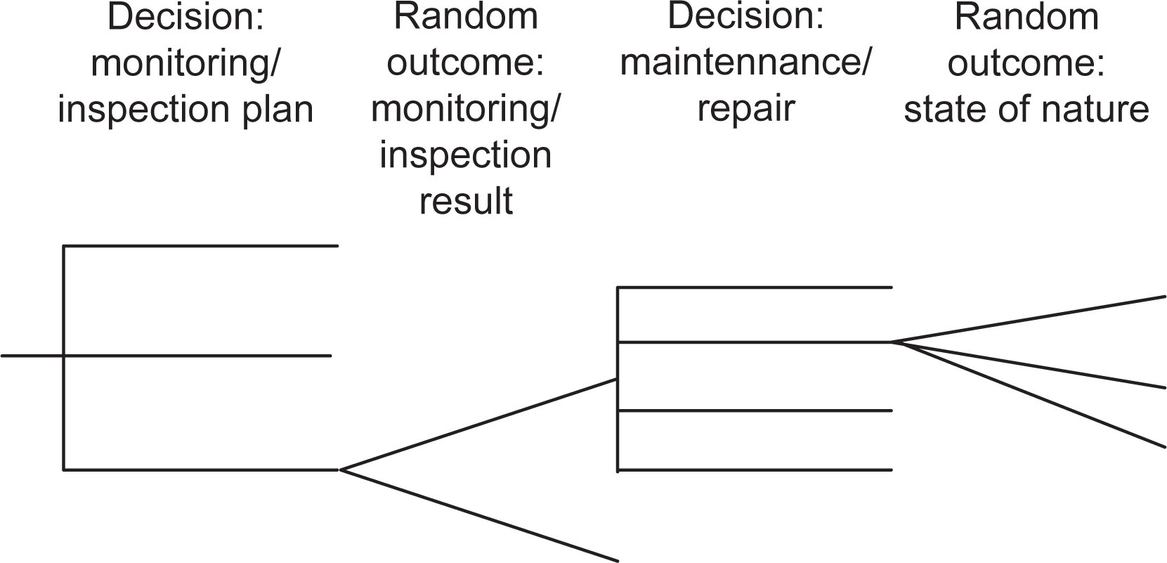
When decisions on inspections and repairs are considered, the decision problem can be illustrated in a decision tree, as shown in Figure 2, where the tree is repeated for each time step. The decisions can be represented by decision rules. In the unreduced case, the decision rules are dependent on all observations from the entire past, and these are unknown when the optimal decision rules are found. An approximation is to use simpler decision rules that do not include the entire past.
2.1. Assessment of Probabilities
In order to use the Bayesian pre-posterior decision analysis, it is necessary to compute the probabilities of failure, probabilities of monitoring results, probabilities of inspection results and probabilities of repair, as they are needed to compute the expected costs. Therefore, probabilistic models are needed for the deterioration process, for monitoring and for inspection.
For the deterioration process, a model for the damage development can be developed, where uncertainties are included. Based on the model, the distribution for the damage size can be found at all time steps. For example, a fracture mechanical model can be used for fatigue, and the parameters for the model can be calibrated based on the design model that is often based on SN models [11]. When monitoring or inspections are available, the probabilities of the different inspection and monitoring outcomes can be evaluated based on the monitoring or inspection model. Furthermore, the probability distribution for the damage size can be updated using Bayesian updating when inspection and monitoring results are available, and thereby, the probability of failure can be updated.
A probabilistic damage model for the damage size at time step i can be formulated as:
For inspections and monitoring, a probabilistic model for the inspection outcome Ii can be formulated as:
2.2. Costs
The costs of inspections, repairs and failures influence the optimal decisions and should be included in the model. Furthermore, the indirect costs due to lost production should be included. Inspections and preventive repairs can be planned during low winds, but in case of failure, there could be a long period with downtime. First, there will be a mobilization period, if spare parts or special vessels need to be ordered, and secondly, the weather might be too harsh for repairs, and it will be necessary to wait until the wave height and wind speed are below the limits for the repair for offshore wind turbines.
3. Methods for Risk-Based Decision Making
As described in Section 2, approximations are generally necessary to solve the decision problem for maintenance. One approximation is to consider only stationary decision rules. Then, the optimization can be performed manually, and there are several approaches for calculating the probabilities, as will be described in Section 3.1. If time-variant decision policies are desired, other approaches can be applied. Sections 3.2 and 3.3 will consider approaches based on limited memory influence diagrams (LIMID) and Markov decision processes.
3.1. Methods with Manual Optimization
For the methods described in this section, the optimization is done manually. That is, the total expected costs are found for various combinations of decision rules, and the optimal set of decision rules is the one yielding the lowest total expected costs. The following methods will be considered:
Decision tree;
Crude Monte Carlo simulations;
Discrete Bayesian network;
Markov chain Monte Carlo simulation;
Simulation in a Bayesian network.
The most simple decision rules are based on a constant or an observed quantity, and those decision rules can easily be implemented in all of the methods. A more complicated option is to use quantities found using Bayesian updating, e.g., the probability of failure. To use that approach, the last option can be applied, simulation in a discrete Bayesian network, or a decision tree can be used to some extent.
3.1.1. Decision Tree
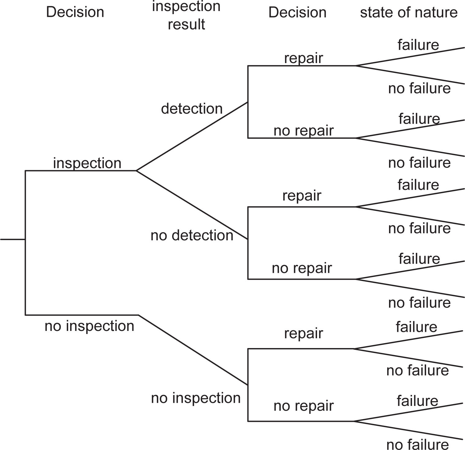
For decision trees, the computation time increases exponentially with the number of time steps, unless there is only one branch. For risk-based inspection planning in the oil and gas industry, this has been solved by using approximations until there is only one branch left to evaluate, as described in [8]. Figure 3 illustrates a typical decision tree for RBI.
A decision rule often introduced is to repair only in case of damage detection at an inspection and, in some cases, to use a threshold for damages that are repaired. Secondly, repaired components are assumed to act as either new components or components with no damage detections. Thirdly, failures are considered to terminate the lifetime of the structure. Finally, the inspections can be made with either a fixed interval or whenever the reliability drops below a certain threshold value. In this way, only one branch in the decision tree continues. In case of preventive repairs, the assumption regarding repaired components determines how the costs are evaluated. In case it acts like a new component, the expected costs are found for lifetimes of all lengths up to the actual lifetime, and the results for shorter lifetimes are used when expected costs are found for longer lifetimes. If it acts like a component with no damage detections, the expected costs for the remaining lifetime are the same for the branch with repair as for the branch with no damage detections, and they can be evaluated as one.
The optimal inspection plan can be found by calculating the expected costs for different inspection intervals or reliability thresholds and choosing the one with the lowest costs. The probabilities needed for the evaluation of the costs are typically found using structural reliability methods, such as FORM (First Order Reliability Method), SORM (Second Order Reliability Method) or Monte Carlo simulation [12].
For offshore wind turbines, many failures happen throughout the lifetime, so failure cannot be considered as a terminal event. However, failed components can be assumed to be repaired and act like preventively repaired components, and the approach could still be used.
3.1.2. Crude Monte Carlo Simulations
The simplest way to assess the expected costs of various maintenance strategies is to run Crude Monte Carlo simulations. N independent samples are drawn from the distribution for each stochastic variable, and simulations are run for various strategies for inspections and repairs. The expected costs can then be found from the mean number of inspections, repairs and failures.
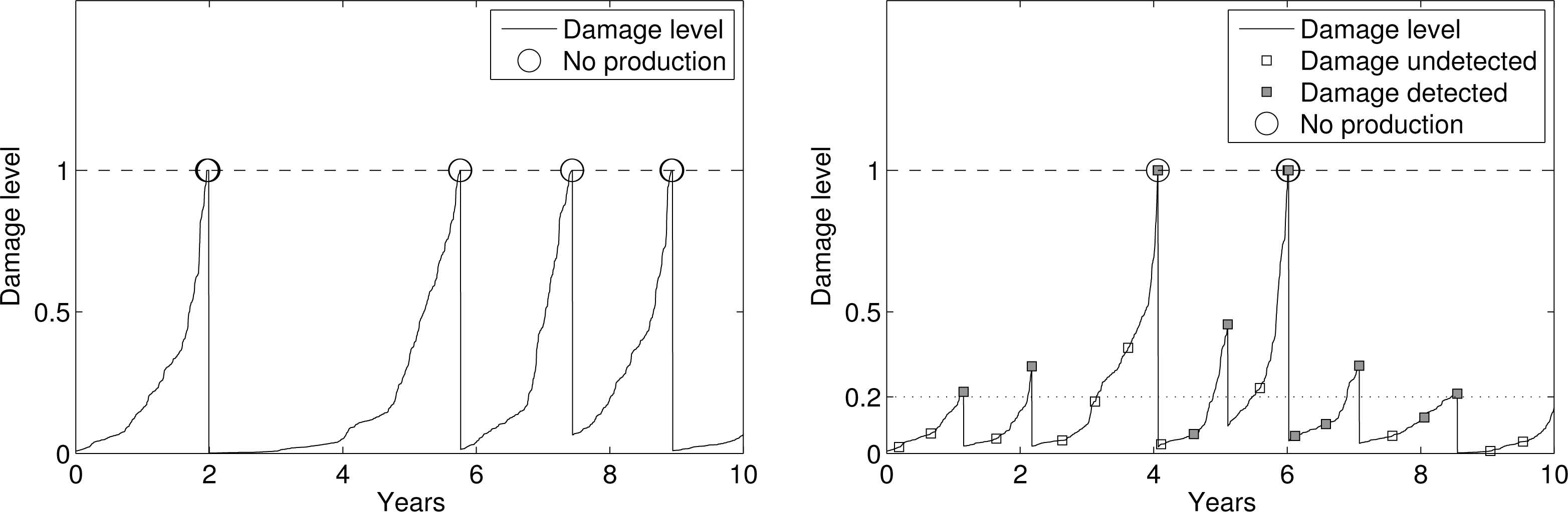
This approach is rather time-consuming and should not be used in cases where the probability of failure is very low, since too many simulations will be needed to give a good approximation of the expected costs. The approach is simple to implement, and an accurate model can be used for, e.g., damage growth. Figure 4 shows an example of simulations with corrective- and condition-based maintenance, respectively. After failure, there is a period with no production of power. When condition-based maintenance is used, there are fewer periods with no production, as some damages are detected during inspections and are repaired preventively. The approach was demonstrated in [13,14].
3.1.3. Discrete Bayesian Network
A Bayesian network is a directed acyclic graphical model consisting of nodes representing stochastic variables and directed links representing causal relationships. For problems with variables that evolve over time, a dynamic Bayesian network (DBN) can be used for the modeling. It consists of a number of time slices equal to the number of time steps in the model, and each slice is connected only to the neighboring slices.
If there is a link from Node A to B, A is called the parent of B and B the child of A. The probability distributions need to be specified for each node, conditional on the parents. For maintenance planning, the decision problem generally contains both continuous and discrete stochastic variables, and often, there will be no closed form solution for the posterior distributions. However, if all nodes are discrete, there are efficient methods for exact Bayesian updating. Therefore, an approach is to discretize all variables, such that those methods can be used.
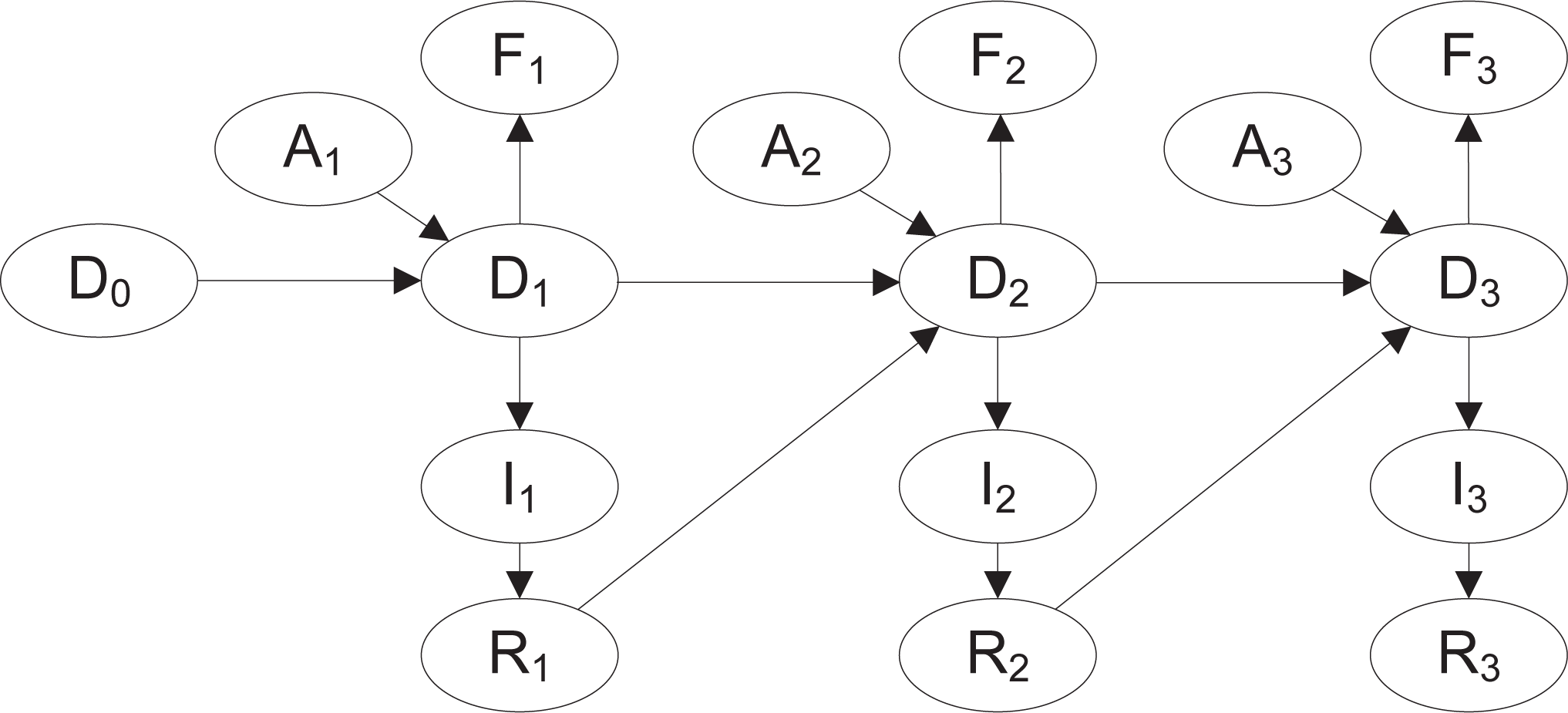
Figure 5 shows an example of a Bayesian network for deterioration modeling. The variables D, A and possibly I are continuous and are discretized in appropriate intervals; see [9,15]. The failure node F is discrete with two states: failure and no failure. Failure is assumed to happen when the damage size reaches the last interval of the node D. The repair node R is also discrete with two states: repair and no repair.
The distributions for the nodes with no parents are found directly by discretizing their continuous distributions. The distribution for the damage node D should be given as a conditional probability distribution:
If the inspection interval is fixed, the step length for time can be set equal to the inspection interval. To optimize the inspection interval, the step length can be reduced, and the nodes I and R can be omitted for time steps with no inspections. The repair policy can be changed by changing the distribution for the repair node R. For a deterministic decision rule, it will contain ones for the event of repair for all inspection outcomes that should lead to repair and zeros for no repair. The network can then be used directly for calculating the expected number of inspections, repairs and failures, and the expected costs can be found by multiplying by the costs for each of them. Different inspection and repair policies can be tried out, and the optimal is the combination yielding the lowest costs.
3.1.4. Markov Chain Monte Carlo Simulation
Another method for statistical inference in a Bayesian network is the Markov Chain Monte Carlo (MCMC) sampling. In the same way as for the discrete Bayesian network, the probability distributions are specified for each variable, conditional on the parents. The Markov Chain Monte Carlo simulation is a simulation technique, where the simulations form a Markov Chain; thus, each set of simulated variables is allowed to depend on the previous set of variables, instead of being independent, as for Crude Monte Carlo simulation. Even though successive sets of simulated variables are correlated, the stationary distribution for the simulated variables can be shown to be the true posterior distribution.
For maintenance planning, the program OpenBugs [16] has been used for MCMC sampling, as the flexibility of the program allows for building models for deterioration processes with inspections, repairs and failures; see [9] for details. The program has various built-in MCMC sampling methods, such as Gibbs sampling, Slice sampling and sampling using the Metropolis–Hastings algorithm, and it selects the most suitable sampling method for each variable based on the model and the available data. The model specifies the relationship between the variables, and both deterministic and probabilistic relationships can be specified. Probabilistic relationships are specified as probability distributions and deterministic relationships as logic functions.
A network similar to the discrete Bayesian network in Figure 5 can be built, and the expected costs can be found for various combinations of deterministic decision rules.
3.1.5. Simulation in Bayesian Network
In the methods considered so far, deterministic decision rules based on constants or observed variables are used. Instead, it could be desirable to use decision rules based on variables found using Bayesian updating, such as the probability of failure. To do so, the crude Monte Carlo simulation can be used in combination with a Bayesian network. For various decision rules, crude Monte Carlo simulations are run. Each time a decision involving Bayesian updating needs to be made, the simulated evidence is put into a Bayesian network, the network is updated and the simulation continues with the decision made using support from the Bayesian network.
As the Bayesian network needs to be updated continuously, the updating should be very fast, so a discrete Bayesian network is most suitable. When the decision rules are to be used in practice, it is again necessary to perform Bayesian updating to use the decision rules.
3.2. Influence Diagrams
An influence diagram is an extension of a discrete Bayesian network representing a decision problem. In addition to the stochastic nodes in a Bayesian network, an influence diagram also contains decision nodes (rectangular) and cost nodes (diamond shaped). To represent the full decision problem, the decision nodes should be dependent on all observations from the entire past. However, this problem is generally intractable, just like the original decision tree, and approximations are necessary.
An approximation is to let the decision depend only on some nodes, instead of the entire past. For this, a limited memory influence diagram (LIMID) has been developed, where the decision policies depend only on the parents of the decision nodes [17]. The decision policies can be time-variant, as the optimal policy is found for each of the decision nodes. The optimal policies are found using a single policy updater algorithm. This algorithm updates one policy at a time, until lower costs cannot be found by changing only one policy. Therefore, the algorithm finds a local minimum, but not necessarily the global minimum. The LIMID should, therefore, be created in such a way that the algorithm will find the global minimum.
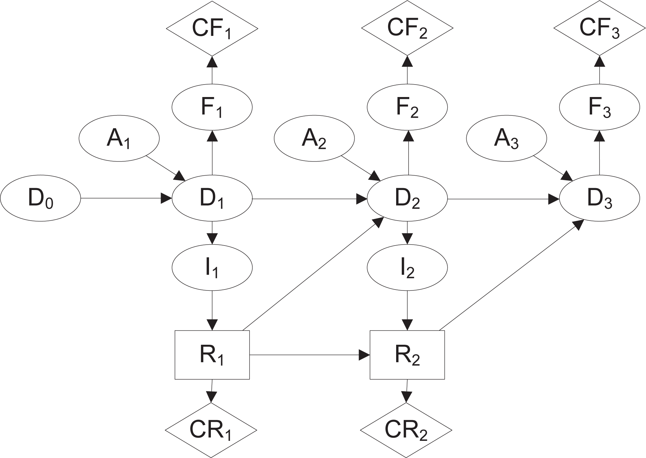
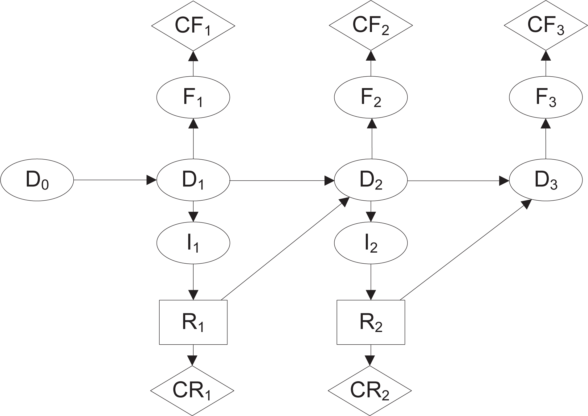
For maintenance problems where a decision needs to be made for each time step, only one type of decision should be modeled to avoid getting stuck at local minima. For example, decisions on repairs could be modeled by decision nodes, and inspections could be scheduled with a fixed interval, as shown in Figure 6. The decision nodes have the most recent inspection outcome, as well as the most recent repair decision as the parent.
If the single policy updating algorithm is run prior to the beginning of the lifetime, the “optimal” policies can be found for the entire lifetime. However, these policies only take the most recent inspection result and the most recent repair decision into account. If, instead, observations are entered into the network throughout the lifetime and the policies are updated each time a decision is made, the entire past is taken into account for the present decision and only future decisions are approximated.
3.3. Markov Decision Processes
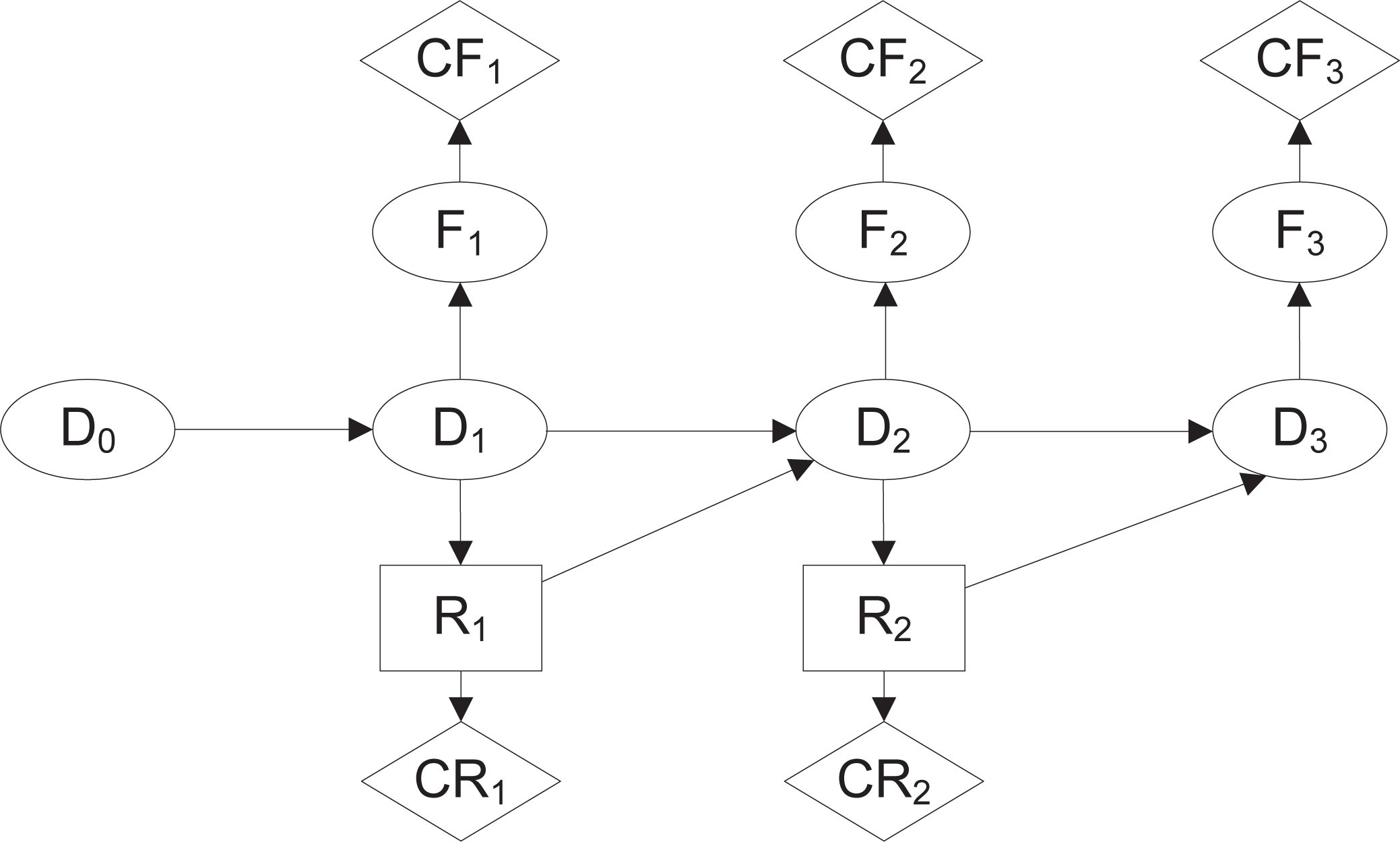
For a Markov process, the future is independent of the past, given the present. This is the case for deterioration models without time-invariant uncertainties, where the future damage development only depends on the present damage size and not the history of damage development. If the damage size is directly observable, the optimal decision only depends on the present damage state, and the decision problem is a fully observable Markov decision process, as illustrated in Figure 7.
This decision problem can efficiently be solved using dynamic programming by exploiting the Markovian assumption [18]. The idea is to calculate the optimal strategy for each possible damage state for each time step, starting at the last time step, and then use the results for later time steps when optimal decisions for former time steps are found. In this way, the computation time is linear with the number of time steps and not exponential, as for the decision tree.
When the damage size is only observable through an indicator, the decision process is a partially observable Markov decision process (POMDP), as illustrated in Figure 8. Here, the damage size is not known for the decision maker, but the same principle can still be used. Instead of finding the optimal decision for each possible damage size, the optimal decision is found for each possible probability distribution for the damage size. In practice, there are infinite possible probability distributions, but the expected costs can be found for a number of grid points, and those results can be used when calculating the expected costs for the former time steps.
Because the decisions are made based on the probability distribution for the damage size, all sorts of information can be used for Bayesian updating of the damage size and thereby be included in the model. Furthermore, more types of decisions can be included. In [19], decisions were made on inspections and repairs, and the distribution for the damage size was updated using monitoring and inspections. However, only three states were used to describe the size of the damage. For more states, the expected costs can be found for grid points for the parameters of an appropriate distribution.
4. Case Study
This section presents a case study where four of the presented optimization methods with different types of decision rules are compared for the same model. The models and costs used in the case are not based on real data, and the case study is only meant to illustrate the difference in results obtained using the methods.
4.1. Model
In the case study, only one damage mode is considered. The damage size is assumed to be continuous and can take values from zero to nine, with values above nine being in the failed state. The damage size is discretized in 10 intervals with lower interval boundaries 0,1,. . . ,9, with the last interval corresponding to failure. Initially, the damage size is within the first interval, and the same is true after a preventive repair and after repair of a failed component. The transition probability is constant for each state, and it is only possible to jump one state during a time step. The mean time to failure is set to 40 years; the time step is one month, and the lifetime is 20 years.
Online monitoring is available with four possible outcomes: no alarm, low alarm, high alarm and failure. The expected value for damages causing low and high alarm is 2.0 and 5.0, respectively, and the coefficient of variation is 1.0 for both. The damage size causing an alarm is considered lognormal distributed. Failures are always detected by the monitoring system. Inspections are modeled in a similar way, and Table 1 shows the possible outcomes for inspections.
The costs are set relative to the cost of an inspection, such that the cost of an inspection is one. The cost of failure is set to 600, including lost production, and the cost of preventive repair is set to 20. The probability of harsh weather for longer than one time step is not included; thus, it is always possible to repair in the same time step where a decision on repair is made or a failure has happened.
4.2. Methods for Decision Making
The methods for decision making considered in this example are:
A, DBN: constant inspection interval and threshold for inspection outcome for repairs.
B, DBN: threshold for monitoring outcome for inspections and threshold for inspection outcome for repairs.
C, simulation in DBN: threshold for the probability of failure for inspections and threshold for inspection outcome for repairs.
D, Markov decision process: the optimal decision for the nearest Weibull distribution is used.
4.2.1. A: Inspection Interval and Inspection Threshold for Repairs
Method A is computationally inexpensive. As all decisions are made based on observed quantities or constants, dynamic Bayesian networks can be applied to find the expected costs directly. The expected costs are evaluated for combinations of number of inspections and thresholds for the inspection outcome for repair decisions.
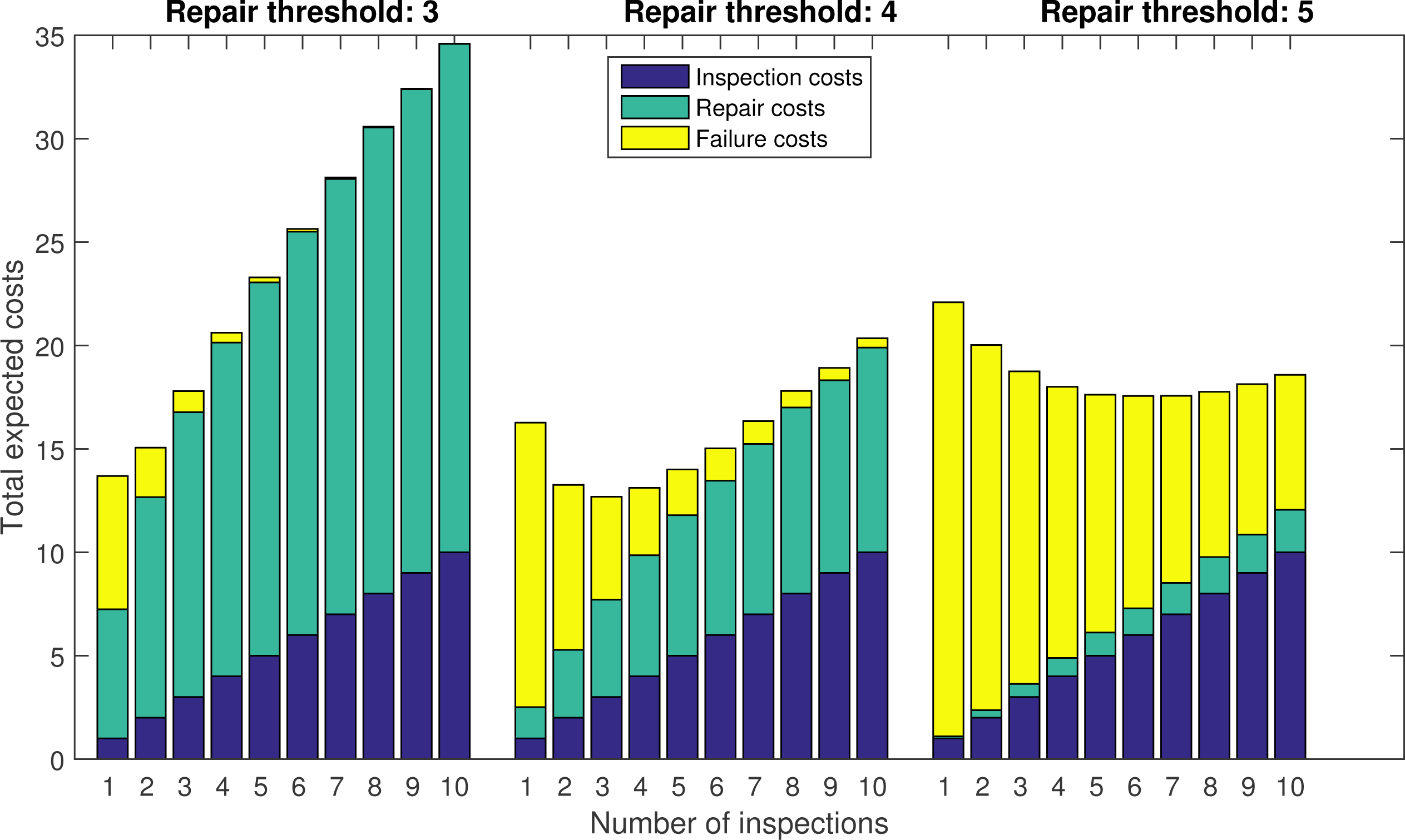
Figure 9 shows the total expected costs for Method A for combinations of number of inspections and threshold for repairs. The lowest costs (12.69) are obtained with three inspections distributed throughout the lifetime of the wind turbine, and a repair threshold corresponding to the inspection outcome of four (significant damage).
4.2.2. B: Monitoring Threshold for Inspections and Inspection Threshold for Repairs
Method B is similar to Method A, except for the decision rule for inspections. The expected costs are evaluated for different combinations of thresholds for monitoring outcome for inspections and thresholds for inspection outcomes for repairs as for Method A. For Method B, the lowest costs (50.05) are obtained at a threshold for inspections at a monitoring outcome of three (high alarm) and a threshold for repairs at an inspection outcome of four (significant damage).
4.2.3. C: Probability of Failure Threshold for Inspections and Inspection Threshold for Repairs
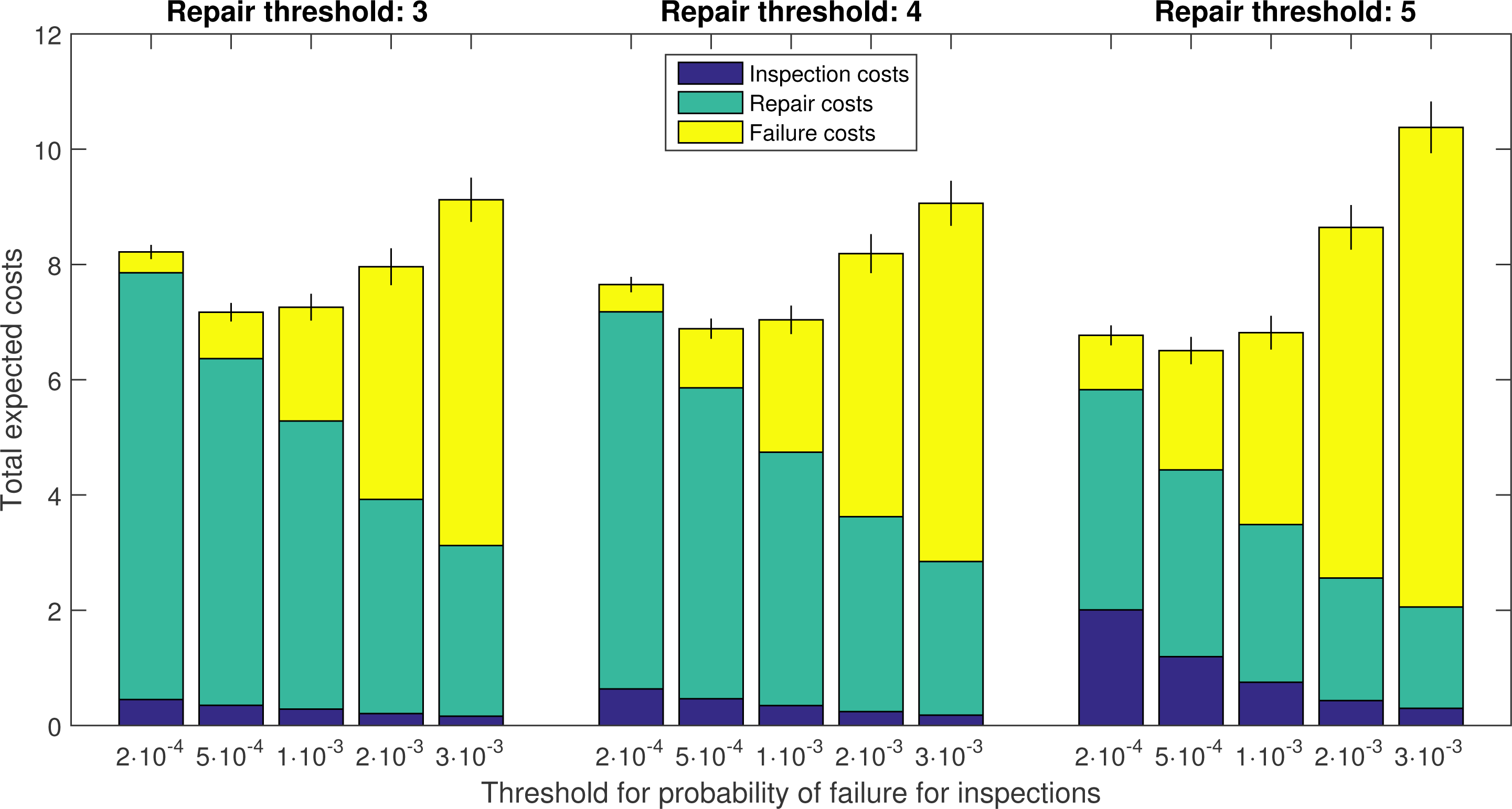
Crude Monte Carlo simulations are necessary to find the optimal decision rules in Method C. The decision rule for inspections are based on the probability of failure within the following time step (one month), evaluated based on the damage model and all previous monitoring and inspection outcomes. The decision rule for repair is based on the most recent inspection outcome.
Figure 10 shows the total expected costs found using Method C for different thresholds for inspections and repairs using 100,000 simulations and 95% confidence intervals for the total expected costs. The lowest costs (6.5) are obtained at a threshold for the probability of failure at 0.0005 per month and a threshold for repairs at an inspection outcome of five (severe damage). However, the result is not very sensitive to changes in the repair threshold.
4.2.4. D: Markov Decision Process
For the Markov decision process, the optimal decisions are in principle found for each time step for each possible probability distribution for the damage size. The grid points for calculating the optimal policies for each time step are found by approximating the distribution by a discretized Weibull distribution with scale parameter a and shape parameter b, truncated before the failure state. For the parameter a, the grid contains values from 0.25 to 11.50 with a step length of 0.05, and for b, the grid contains values from 0.50 to 5.50 with a step length of 0.125. This results in 9267 probability distributions to be evaluated at each time step, including the probability distribution for a failed component. The calculations are done in a recursive manner, where the expected costs for the remaining lifetime are found based on the grid point closest to the current probability distribution for the damage size. The criterion for the selection of the grid point is based on a least squares comparison based on the discrete cumulative distribution function.
The decision on inspection is made based on the probability distribution for the damage size after monitoring, and the repair decision is made based on the probability distribution for the damage size updated using the inspection outcome, if relevant. The decision policies for inspections and repairs depend on time and on the probability distribution for the damage size after monitoring. This probability distribution is approximated by the nearest Weibull distribution in the grid; thus, the inspections policies depend on time, as well as scale and shape parameter a and b. The repair policies additionally depend on the inspection outcome.
Figure 11 illustrates the policies for inspections and repairs five years into the lifetime. The plot shows the difference in the costs between the decision alternatives inspection and no inspection and repair and no repair, respectively. Positive values indicate that the action is recommended.
When the optimal policies are found, the expected costs are also found for the entire lifetime. However, they are found based on the Weibull approximation and could be misleading. Therefore, crude Monte Carlo simulations have been applied to assess the expected costs when applying this approach. The computations for assessing the costs are similar to the method with simulation in a DBN, as only the decision rules differ. The total expected costs using method D is found to 6.6, evaluated based on 100,000 simulations.
4.3. Comparison
Figure 12 shows the expected costs obtained by each of the four methods. Methods A and B are the simplest to implement, as they use only simple decision rules. Even though Method B includes more information than Method A, as it includes monitoring, it performs much worse, since the costs are four-times larger. The reason is the large uncertainty on the monitoring outcome, as high alarms are obtained relatively often and, consequently, too many inspections are performed. Method C also includes monitoring, but the uncertainty is considered, as the monitoring outcome is used to update the probability distribution for the damage size, thereby changing the estimate of the probability of failure in the following time step. Therefore, Method C performs better than Methods A and B. Method D goes even further and uses the updated probability distribution for the damage size for both the decision on inspections and repairs, and repairs can be performed without first performing an inspection. The costs obtained by Method D are similar to Method C.
5. Discussion
The main limitation of the approaches with manual optimization is that all decision rules need to be set up in a deterministic manner prior to the evaluation of the total expected costs. This can be done for various combinations of decision rules for inspections and repairs, and the optimal decision rules are found. In principle, the decision rules do not have to be stationary. They could be time-variant, as long as the variation is set as a deterministic decision rule.
Time-variant decision policies are relevant near the end of the life-time of the wind turbine and when seasons are included in the model. Near the end of the lifetime, expensive repairs will not be profitable if the income from the produced power is less than the cost of the repair. This is considered in the decisions for the LIMID approach and for the Markov decision process. If the possibility of harsh weather is included in the model, it can be relevant to include seasons. During the winter, it is more likely that repairs cannot be made, and therefore, more preventive repairs could be made during the summer, to reduce the risk of downtime. For the Markov decision process, seasons can easily be implemented, as shown in [19]. For the LIMID approach, it could also be included by adding a stochastic node for repairs being possible between the decision node for repair Ri and the node for the damage size at the following time step Di+1. This node should then be the parent for the decision node at the following time step Ri+1 instead of Ri.
In the basic decision model presented in Section 2, information was assumed to be available from inspections only. Only this information is taken into account when using decision rules for repairs based on the inspection outcome. Sometimes, monitoring is also available and could give relevant information to include in the decision problem. The monitoring result could be used as input for the decision rule for making an inspection. However, for the methods with decision rules based on an observed quantity, the monitoring information would not be used when the decision on repair is made. However, it can be taken into account in the other methods. For the LIMID approach, future monitoring results are not taken into account in the future decisions, but past monitoring results can be entered into the network and taken into account for the current decision. For the Markov decision model, monitoring can be implemented, and the information is fully considered for all decisions. If the probability of failure is used for the decision rule and the optimal decision rule is found using simulation in a Bayesian network, it is possible to use monitoring results to update the probability of failure.
For the decision tree, the probability of failure can also be used as a decision rule for when to make inspections. However, monitoring information cannot be used to update the probability of failure in this case, as it would create a new branch for each possible inspection outcome, and the problem would be computationally infeasible. The only information used for updating the probability of failure for the decision tree is whether or not a repair has been made. Because the event of repair is coupled to the inspection result through a deterministic decision rule, the inspection model influences the updating of the probabilities.
The deterioration model presented in Section 2.1 is a Markov model, as the damage size only depends on the damage size on the previous time step and a time-independent model parameter. However, deterioration processes are generally not Markovian if time-invariant uncertainties are present. Deterioration processes can still be modeled using the same approach, as long as the time-invariant uncertainties are modeled with a parameter included in the model. The time-invariant parameter could influence the rate of damage development. If the damage size was observed at several times, the uncertainty on the parameter would be reduced and the prediction of future damage development would be more accurate. In this way, past information can be used to update the time-invariant parameter, and then, the future is independent of the past, given the present damage size and the present value of the time-invariant parameter.
For the Bayesian network models, a time-invariant parameter can easily be included. However, it will not be important when using a decision rule based on an observed quantity. If the decision rule is based on the probability of failure or if a LIMID is used, the information is exploited. The information can also be retained after repairs or failures, and more knowledge of the deterioration process can hereby be gained during the lifetime of the wind turbines.
For the Markov decision process, the optimal decision is found for each time step for each possible distribution for the damage size. To include time-invariant uncertainties, the optimal decision could be found for all possible joint probability distributions for damage size and for a parameter modeling the time-invariant uncertainty. Although possible, this would significantly increase the computation time.
For the models considered in this paper, the decisions are made by only considering one component in one wind turbine. In reality, turbine operators will often have several wind farms containing many wind turbines, each consisting of several components. In many cases, lower costs can be obtained by applying a system approach. For example, there could be joint uncertainties between turbines in a wind farm, and hereby, observing one turbine gives information about the others. Furthermore, the costs could change if a system approach is applied. When large vessels are needed for major repairs, the mobilization costs can be significant, so it could be cheaper to cluster repairs. If all components in all wind turbines were to be united in one decision model, it would not be possible to find an optimal solution, as the problem is too complex. However, approximations of system effects could be taken into account when appropriate. For example, if a large vessel is ordered for a major repair, one could ask if other components should be repaired preventively at the same time, when no additional mobilization costs need to be paid. This can easily be implemented for the Markov decision model [19].
6. Conclusions
The aim of the work was to develop methods for risk-based decision-making for offshore wind turbines, such that available information can be exploited.
For the methods with decision rules based on a constant or an observed quantity, only one input can be used for each decision. For example, monitoring information could be used to determine when to make inspections, and inspections could be used to determine when to make repairs. In practice, the decisions are often made on that basis, and these methods could help find the optimal threshold values for inspections and repairs. Additionally, a result like this is easy to use for the operators. However, the methods lack the ability to use older monitoring and inspection results to predict the future damage development.
For the other methods, several types of information from monitoring and inspections can be used to update the damage model and the probability of failure. Here, the operators need a program in which they can enter the observations, and the program will then tell them the optimal decisions. This needs to be done every time a decision is made. For the LIMID and the Markov decision process, the program could also give the expected costs in the remaining lifetime for each decision alternative, and thereby, the decision maker can let practical things determine the decision if the costs are almost equal for each decision alternative.
The method based on the Markov decision process is in theory the most accurate, since all information is taken into account, and the optimal decisions are used for future decision and not approximated, as with the LIMID. Furthermore, several types of decisions can be included, and the decision policies can be time variant. In principle, the method could be further developed to include time-invariant uncertainties, and if that can be successfully implemented in practice, the method could be the basis for a very strong decision support tool.
Acknowledgments
The work presented in this paper is part of the project “Reliability-based analysis applied for reduction of cost of energy for offshore wind turbines” supported by the The Danish Council for Strategic Research, Grant No. 2104-08-0014. The financial support is greatly appreciated.
Author Contributions
The main idea for the paper was proposed by Jannie Sønderkær Nielsen, and she wrote the first draft of the paper. John Dalsgaard Sørensen thoroughly reviewed the paper.
Conflicts of Interest
The authors declare no conflict of interest.
References
- Engels, W.; Obdam, T.; Savenije, F. Current Developments in Wind - 2009; Technical Report ECN-E–09-96; Energy research Centre of the Netherlands: Petten, The Netherlands, 2009. [Google Scholar]
- Rademakers, L.; Braam, H.; Zaaijer, M.; van Bussel, G. Assessment and optimization of operation and maintenance of offshore wind turbines. In Proceedings of the EWEC 2003, Madrid, Spain, 16–19 June 2003.
- Rademakers, L.; Braam, H.; Obdam, O.; Frohböse, P.; Kruse, N. Tools for estimating operation and maintenance costs of offshore wind farms: State of the art. Proceedings of the EWEC 2008, ECN-M–08-026, Brussels, Belgium, 31 March–3 April 2008.
- Philips, J.; Morgan, C.; Jacquemin, J. Evaluating O&M strategies for offshore wind farms through simulation—the impact of wave climatology. In Proceedings of the OWEMES 2006, Rome, Italy, 20–22 April 2006.
- Stratford, P. Assessing the financial viability of offshore wind farms. In Proceedings of the EWEC 2007, Milan, Italy, 7–10 May 2007.
- JCSS, Risk Assessment in Engineering—Principles, System Representation & Risk Criteria; Technical Report; Joint Commitee on Structural Safety: Zurich, Switzerland, 2008; ISBN: 978-3-909386-78-9.
- Faber, M.H. Risk-based inspection: The framework. Struct. Eng. Int.: J. Int. Assoc. Bridg. Struct. Eng. (IABSE) 2002, 12, 186–194. [Google Scholar]
- Straub, D. Generic Approaches to Risk Based Inspection Planning for Steel Structures. Ph.D. Thesis, Swiss Federal Institute of Technology, ETH Zurich, Zurich, Switzerland. 2004. [Google Scholar]
- Nielsen, J.S. Risk-Based Operation Maintenance of Offshore wind Turbines. Ph.D. Thesis, Department of Civil Engineering, Aalborg University, Aalborg, Denmark. 2013. [Google Scholar]
- Raiffa, H.; Schlaifer, R. Applied Statistical Decision Theory; Harvard University: Cambridge, MA, USA, 1961. [Google Scholar]
- Nielsen, J.J.; Sørensen, J.D. Risk-based operation and maintenance using Bayesian networks: Influence of epistemic uncertainties. Proceedings of the 24th International Congress on Condition Monitoring and Diagnostic Engineering Management (COMADEM2011): Advances in Industrial Asset Integrity Management, Stavanger, Norway, 30 May–1 June 2011.Singh, M., Rao, R.B.K.N., Liyanage, J.P., Eds.; Publishing Services PL: Kolkata, India, 2011; pp. s.639–s.649.
- Madsen, H.O.; Krenk, S.; Lind, N.C. Methods of Structural Safety; Dover Publications: Mineola, NY, USA, 2006. [Google Scholar]
- Nielsen, J.J.; Sørensen, J.D. On risk-based operation and maintenance of offshore wind turbine Components. Reliab. Eng. Syst. Saf 2011, 96, 218–229. [Google Scholar]
- Nielsen, J.J.; Sørensen, J.D. Risk-based operation and maintenance planning for offshore wind turbines. In Proceedings of the Reliability and Optimization of Structural Systems: Proceedings of Reliability and Optimization of Structural Systems, Tum, München, Germany, 7–10 April 2010.Straub, D., Ed.; C R C Press LLC: London, UK, 2010; pp. 131–138.
- Straub, D. Stochastic modeling of deterioration processes through dynamic bayesian networks. J. Eng. Mech 2009, 135, 1089–1099. [Google Scholar]
- Lunn, D.J.; Thomas, A.; Best, N.; Spiegelhalter, D. WinBUGS—A Bayesian modelling framework: Concepts, structure, and extensibility. Stat. Comput 2000, 10, 325–337. [Google Scholar]
- Lauritzen, S.L.; Nilsson, D. Representing and solving decision problems with limited information. Manag. Sci 2001, 47, 1235–1251. [Google Scholar]
- Dasgupta, S.; Papadimitriou, C.; Vazirani, U. Algorithms; McGraw-Hill: New York, NY, USA, 2006. [Google Scholar]
- Nielsen, J.S.; Sørensen, J.D. Maintenance optimization for offshore wind turbines using POMDP. In Proceedings of the Reliability and Optimization of Structural Systems: Proceedings of the 16th Working Conference on the International Federation of Information Processing (IFIP) Working Group 7.5 on Reliability and Optimization of Structural Systems, Yerevan, Armenia, 24–27 June 2012.Der Kiureghian, A., Hajian, A., Eds.; American University of Armenia Press: Yerevan, Armenia, 2012; pp. 175–182.


| State | Description | Mean | COV |
|---|---|---|---|
| 1 | no detection | - | - |
| 2 | mild damage | 2.0 | 1.0 |
| 3 | some damage | 4.0 | 0.8 |
| 4 | significant damage | 6.0 | 0.6 |
| 5 | severe damage | 8.0 | 0.4 |
| 6 | failure | 9.0 | 0.0 |
© 2014 by the authors; licensee MDPI, Basel, Switzerland This article is an open access article distributed under the terms and conditions of the Creative Commons Attribution license (http://creativecommons.org/licenses/by/3.0/).
Share and Cite
Nielsen, J.S.; Sørensen, J.D. Methods for Risk-Based Planning of O&M of Wind Turbines. Energies 2014, 7, 6645-6664. https://doi.org/10.3390/en7106645
Nielsen JS, Sørensen JD. Methods for Risk-Based Planning of O&M of Wind Turbines. Energies. 2014; 7(10):6645-6664. https://doi.org/10.3390/en7106645
Chicago/Turabian StyleNielsen, Jannie Sønderkær, and John Dalsgaard Sørensen. 2014. "Methods for Risk-Based Planning of O&M of Wind Turbines" Energies 7, no. 10: 6645-6664. https://doi.org/10.3390/en7106645