A Review of Methodological Approaches for the Design and Optimization of Wind Farms

Abstract

This article presents a review of the state of the art of the Wind Farm Design and Optimization (WFDO) problem. The WFDO problem refers to a set of advanced planning actions needed to extremize the performance of wind farms, which may be composed of a few individual Wind Turbines (WTs) up to thousands of WTs. The WFDO problem has been investigated in different scenarios, with substantial differences in main objectives, modelling assumptions, constraints, and numerical solution methods. The aim of this paper is: (1) to present an exhaustive survey of the literature covering the full span of the subject, an analysis of the state-of-the-art models describing the performance of wind farms as well as its extensions, and the numerical approaches used to solve the problem; (2) to provide an overview of the available knowledge and recent progress in the application of such strategies to real onshore and offshore wind farms; and (3) to propose a comprehensive agenda for future research.

1. Introduction

The number, size and complexity of wind farms have been steadily increasing over the past few years as consequence of the ambitious target of producing a larger share of energy from the wind [1,2,3]. This has resulted in a remarkable development in the design of large-scale wind energy conversion systems, which in turn have improved the wind energy economies of scale. Proper wind farm planning has major positive economic impacts for both wind farm investors and developers. However, the problem is not only complex from the technological point of view, but is also subject to an undesirable degree of uncertainty that affects the potential profitability of the project during its expected operational lifetime. As a consequence of the inherent risk, both the required investments and the payback period might be too large to the point of economic unviability. Therefore, detailed planning, modeling and optimization are required to guarantee both technical feasibility and financial competitiveness compared to other conventional forms of energy conversion.

In the early 1970s, important factors such as the worldwide social pressure for denuclearization spurred governments, utilities and the scientific community to explore the potential of wind power for large-scale electricity generation. The first scientific works related to the interactions of Wind Turbines (WTs) in arrays appeared in 1974 [4,5,6,7,8,9,10], marking the beginning of successive paradigm shifts in WT wake (see Section 2.2.1 for a detailed description) modeling and WT array layout optimization. The interactions between WTs through wakes were initially modelled as an equivalent increase in surface roughness which modified the Earth’s boundary layer due to the WT-induced drag. Based on this coarse wake-interaction modeling, it was concluded that quite large separations between WTs were required to avoid significant wake-based energy losses. In the subsequent years, staggered equally-spaced (or grid-like) siting schemes were slowly adopted as a rule-of-thumb by wind farm designers [11,12,13,14,15,16,17]. In the late 1970s and the early 1980s, just after the construction of the world’s first electricity-generating wind farm in New Hampshire (USA) in 1980, the first engineering wake models [18,19,20,21,22,23,24], mostly based on flow momentum conservation and linearized far wake expansion assumptions (with the notable exception of the Larsen [25] and Ainslie [26] models), appeared, laying the groundwork for the first study on Wind Farm Design and Optimization (WFDO) [27], which aimed at optimizing the spacing between WTs in a linear array by using a generalized reduced gradient method that maximized the total power conversion of the array. The maximum achieved increase in power conversion for the given generic study case was 1.29% compared to an equally-spaced linear array. At first glance, this might appear to be a poor improvement, however, a mere one percent improvement in electricity output would result in large additional revenues over the typical 20-year lifetime of wind farms. Seven years later, the classic work of Mosetti et al. [28] on WFDO appeared, leading to significant improvements in both the description of the wind farm performance (the minimized objective metric was the cost of power conversion—see Section 4.5 for misconceptions) and the numerical approach to tackle the problem (a population-based metaheuristic; the Simple Genetic Algorithm or SGA). After that, many authors have performed a significant amount of contributions of variable complexity along two main tracks: (1) a track related to improving the performance modeling of wind farms (i.e., by considering the inclusion of complex sub-models for financial prospection, aerodynamics and airflow physics, structural fatigue and degradation, electrical system and grid interconnection, environmental impact and uncertainty among others); and (2) a track related to the development and testing of different numerical solution procedures. However, individual approaches in the literature do not completely respond to the needs of the wind farm designers, since these tracks were treated and developed separately. In this regard, the interested reader might be disoriented, since it is still unclear which models, objectives and numerical schemes are best suited for application in the treatment of the WFDO problem. To overcome this issue, this work reviews and examines the most promising, effective, recurring models and solution methods, highlighting their strengths and weaknesses, and proposes a research agenda. The present work is structured as follows: Section 2 summarizes the most important concepts involved in the wind farm design process. Section 3 analyses the most prominent literature related to the WFDO problem, including the state-of-the-art modeling approaches and solutions methods. Section 4 outlines the research needs and trends in the WFDO problem. Finally, Section 5 presents the overall conclusions.

2. Overview of the Basic Concepts of Wind Farm Design and Optimization

The design and optimization of wind farms is a complex multidisciplinary topic that can proceed in different ways. The starting point are the existing guidelines and international standards, which give a clear overview of the important factors that affect the decision making of the wind farm designer. The present section describes these factors, the design variables and the formal definition of the WFDO problem.

2.1. Wind Farm Planning—Guidelines and Standards

In general, it is recommended to specify and design wind farm projects in accordance with the state-of-the-art standards of the International Electrotechnical Commission (IEC) [29] and the technical guidelines proposed by international wind energy associations. Some examples include, but are not limited to:

-

The European Wind Energy Association (EWEA): European Best Practice Guidelines for Wind Energy Development [30].

-

The American Wind Energy Association (AWEA): Wind Energy Siting Handbook [31], the AWEA fact sheets and the standards for wind energy industry [32].

-

The British Wind Energy Association (BWEA or RenewableUK): Best Practice Guidelines for Wind Energy Development [33].

-

Global Wind Energy Council (GWEC): Global Wind Reports (2006–2012) [34].

-

Sustainable Energy Authority of Ireland (SEAI): How to develop a Wind Farm [35].

-

Wind Energy Handbook, Chapter 9: Wind-turbine Installations and Wind Farms [36].

Four general stages for wind farm planning and development are briefly summarized next:

(1) Wind Farm Site Selection. The siting process [37,38,39,40,41] refers to the investigation of an area/region/district with the purpose of selecting the best location (site) for a wind farm. Wind farms are very versatile and can be integrated successfully into many types of landscapes, from agricultural fields to mountain ridges, among others. The selection of the wind farm location is commonly based on a hierarchy scheme including three general factors: (1) the available infrastructure (i.e., accounting for the current capacity of the electrical, civil engineering and communication infrastructure and its expansion plans); (2) the environmental suitability (e.g., accounting for restricted areas such as natural protected areas or bird conservation areas); and (3) the wind resource. The wind resource quantification [42,43,44,45] is based on long-term records (each record being a 10-min averaged measurement obtained from sampling with a frequency of 1 Hz or higher) of atmospheric variables exhibiting temporal and spatial variations: wind speeds [m/s] at different heights, wind directions [°] at different heights, solar radiation [W/m²], temperatures [°C] at different heights, pressure [Pa], relative humidity [%], rain fall [mm], and sometimes even air quality. Since atmospheric variables are considered to be random on nature, further analyses are performed to study its statistical characteristics (e.g., determine its probability density functions), which allow the wind farm designer to quantify expected values at the potential wind farm site. Additional information that helps the designer to dimension the loads and stresses the potential WT will undergo while operating at the site can be obtained from statistical-dynamical analyses, which include the following measured variables: local ambient turbulence intensity [%], power and turbulence spectra and coherences, mean and maximum gusts [m/s], rain/ice/snow/hail [%], chemical effects (related to corrosion by salts and/or soiling), and atmospheric stability cycles [36]. In engineering practice, wind farm designers usually calculate the local 3D wind field of the site by means of commercial packages [46,47,48,49,50,51,52] that implement and numerically solve the governing equations of fluid mechanics. Different levels of sophistication exist for such calculations, with the approach that considers the Reynolds Averaged Navier-Stokes (RANS) equations, complemented with turbulence models, being widely used. It has been shown that the RANS-based models’ predictions provide reasonable agreement with the experimental data measured at sites with complex topography [53]. The micro-scale flow modeling is usually based on high-resolution maps representing the topography, obstacles and roughness of the region. The output wind field is convoluted numerically with the resulting statistical distributions of the 10-min averaged wind speed measurements at different heights and wind directions, resulting in averaged wind resource maps at different heights, which are the base for the wind farm planning process. Other sources of information such as Mesoscale modeling and the Measure–Correlate–Predict (MCP) techniques [36,42] could also provide valuable information of the local atmospheric behavior and the wind resource potential.

(2) Wind Farm Design. The wind farm sizing refers to the process of designing the size of the wind farm in terms of the constrained land area and its potential capacity. The wind farm size will be a function of many factors including the expected power demand from the energy consumers. The wind farm layout design or micro-siting process refers to the design of: (1) a configuration or arrangement of the individual WTs (specified by locations on spatial coordinates (x, y, z) down to 1 m in resolution); (2) their electrical interconnections; and (3) the auxiliary communication and civil engineering infrastructure within the selected site. The optimal design thus results from an optimization given all economic, environmental, technical and social conditions and constraints by using a mono- or multi-objective criteria. During the wind farm micro-siting process, economic simulations, accounting for all available incentives, are performed with the aim of quantifying the expected economic profits of the project while assuming all energy and environmental regulations to be satisfied. Once the economic feasibility of a preliminary project is determined, land owners are contacted and asked for participation in the project by hosting WTs on their land. Land owners receive incomes (royalty fees) from renting their land and usually receive a percentage of the gross income generated by the project, and extra compensations if roads or other infrastructure are built on their terrain. Depending on the landowner’s participation [54], a wind farm redesign could be required. The legal, leasing and planning application processes are not straightforward and may take a significant amount of time. In addition, wind energy best practices for community engagement and public consultation encourage wind farm designers to develop community outreach programs. In this sense, a significant amount of money is spent during the wind farm design process even without any guarantee that the project can be built.

(3) Energy Regulatory Framework. The energy regulations depend on the country where the project is to be developed. The wind farm designer must be aware of the legislation regarding the production, transmission, transformation and marketing of the electricity, which in turn define the potential profitability of the project. In addition, the wind farm designer must act in accordance with the local and national development plans and policies and the electricity market.

(4) Financing and Funding. Once a complete design and organization is performed, the wind farm developer must have access to funds through banking institutions or special financial organizations. The acceptance/rejection of the funding will depend on several factors such as the results from the wind resource assessment, the Power Purchase Agreements (PPAs) for the energy to be converted and supplied, the full planning permissions, feasibility studies, electrical interconnection and construction agreements, banking/economic climate and insurance against natural disasters among other factors [36]. In this sense, the uncertainty on the project revenue is one of the most important factors determining a successful financing.

The present work focuses on describing in detail the approaches used to develop the second stage of the wind farm planning process, where technical and optimization challenges are commonly encountered. It should be noted that topics regarding the design and optimization of WTs and the optimal control of WTs and wind farms were disregarded during the development of this work and should be considered as important problems to be treated. A comprehensive description of the most important factors influencing the wind farm design process is presented in the next section.

2.2. Adverse Factors and Conflicting Objectives

Determining the best wind farm design involves many design trade-offs [55,56] that must be balanced. The set of factors that most affect the micro-siting process are briefly described next, while the state-of-the-art modeling approaches to account for their side effects are presented in Section 3.

2.2.1. Wind Turbine Wakes

The wake of a WT [57,58,59] is a volume of affected flow that is characterized by a reduced streamwise velocity, high vorticity and increased levels of turbulence compared to the free stream airflow. The consequences of operating WTs in the wakes of obstacles (e.g., WTs, meteorological masts or buildings) have been reported based on field experience: (1) Overall power losses up to 41% may occur, where the precise loss figures depend on the inter-WT distances, wind direction, site complexity (e.g., onshore, offshore), turbulence intensity and WT type, among other relevant factors [60,61,62,63,64,65,66,67,68]; (2) Enhanced fatigue loads of up to 80% [58] that drastically reduce the lifespan of the WT and significantly increase the Operation and Maintenance (O&M) costs. In particular, operating a WT under partial wake conditions (i.e., only a fraction of the rotor of the downwind WT operates in the wake of upstream WTs) results in higher fatigue loads in contrast with operating a WT under full wake conditions as pointed out by Seifert et al. [69], where the blade root bending flatwise, the main shaft torque and the tower head bending moment-based fatigue loads are the most affected. In addition, the WT induced turbulence intensity may not only reduce the power output of the downstream WTs but can also cause dynamic loading and increased levels of noise which, in the long run, lead to blade damage and higher O&M costs. Moreover, wind farm wakes produce important disturbances in the atmospheric boundary layer, thus they can potentially affect neighboring wind farms [70,71,72,73].

WT wakes have special relevance for the wind farm design process, as it is the single factor that accounts for the largest energy losses [58,60,61,63,68]. Consequently, the adequate positioning of each WT within the wind farm site is one of the factors that most influences the profitability of a project throughout its operational lifetime.

2.2.2. Wind Farm Infrastructure

One of the most important prerequisites for a wind project is that there should be enough electrical, civil engineering and telecommunication infrastructure, so the project will not incur in large additional expenses [74,75,76] by building auxiliary infrastructure, which in turn might lead to economical unviability.

The wind farm electrical infrastructure is mainly composed of substations containing step-up transformers, Medium Voltage Alternate Current (MVAC) collection lines and High Voltage Alternate Current (HVAC) or High Voltage Direct Current (HVDC) transmission lines. Typically, each WT contains a transformer that increases the generated voltage (e.g., 220 V~3 kV) to the MVAC collection system voltage (e.g., 3 kV~60 kV). The MVAC collection system is in turn connected to a large capacity transformer that raises the voltage to the HVAC or HVDC transmission system voltage (e.g., 69 kV~161 kV) [77].

In practice, several WTs can be connected to the HVAC or HVDC transmission system by sharing a common MVAC collection line circuit. This strategy has proven to reduce the cable length requirements at the expense of increasing the cable size (cross sectional area) in order to meet capacity constraints [77,78,79,80,81]. The MVAC collection system layout depend on the wind farm layout, where WTs can usually be interconnected in a modular fashion, while accounting for the power lines capacity, to produce a combined power output which can be either increased or decreased through the addition or subtraction of WTs at the different stages of the electric network implementation. For security reasons, all the electrical components are typically over dimensioned (e.g., by 30% above the expected rated capacity) since they are very sensitive to variations in the local climate and to electrical instabilities derived from the main electrical system, among other factors, which in turn can produce significant impacts on their performance [82]. The cable size is typically determined based on an economic analysis that in turn depends on the amount of current the cable can transport without overheating, which is a consequence of the Joule-based power losses. Fixed costs are higher for large cross sectional cables, but Joule losses are lower since they have lower electric resistance [55,77,78,79,80,81,83].

The size and location of the wind farm might lead to the problem of finding suitable electrical interconnection points, which must have enough capacity to handle the energy delivered from the wind farm. In cases where the distance between the electrical interconnection point and the wind farm is large (e.g., around 100 km [55,84]) HVDC transmission lines may become more technologically and/or economically convenient than the conventional HVAC transmission lines [85]. However, the decision of using HVDC transmission lines is stressed by the fact that it is generally difficult to get permission and funds to build new overhead lines and/or substations and, although losses are low for HVDC transmission lines, there are added losses due to the Voltage Source Converter (VSC) components, which are typically difficult to quantify. The decision of using one type of transmission line or another (AC or DC) [85] is mostly based on the amount of reactive power generation and on the amount of Joule-based power losses, which depends on the transmission line length, transmission voltage and the rated power among other factors [78,80,82,85,86,87,88,89,90,91]. Therefore, interconnections between the wind farm and the main electric system and interconnections between WTs within the wind farm must be planned with the aim of reducing reactive power generation, power losses and total costs.

The available civil engineering infrastructure should provide route access (e.g., through highways, paved/unpaved roads, tunnels, bridges, railways, etc.) to the wind farm site. It is also desirable to have airports and/or seaports nearby to improve logistic operations during the construction process. Additionally, it should provide a way (e.g., radio frequency-based, telecommunication, Internet-based, wired connection-based or satellite connection-based) through which important information (e.g., wind resource and wind farm real-time operation) can be consulted and monitored, however it mostly depends on the coverage of the local network service providers. Civil engineering and telecommunication infrastructure is commonly not encountered within the wind farm potential areas, thus the wind farm designer usually incur additional expenses [74,76] by building auxiliary infrastructure (e.g., suitable auxiliary roads), which depends exclusively on the wind farm layout, local orography and restricted areas.

2.2.3. Environmental Impacts

Although the World Health Organization (WHO) recognizes wind energy as the power conversion technology with the lowest impacts (during construction and operation) on human health and the local environment [92,93,94,95,96] precautions must be taken during the wind farm design process. Environmental impacts can be defined as all the potential impacts the wind farm will produce in the environment of the site during its construction and while operating. Environmental Impact Assessments (EIAs), which must be in compliance with existing guidelines proposed by national Environmental Affairs Agencies (EAA), should in general include the description and study of the impacts on the air, water and soil. In addition, EIAs should study the effect of possible pollution emissions and their distributions in space and time, noise generation, shadow flicker issues, visual impact and the impacts on wildlife and biodiversity. Examples of EIA guidelines are the United Nations Environment Programme (UNEP) guidelines [97] and the International Finance Corporation (IFC) performance standards on environmental and social sustainability [98]. The environmental factors that most affect the micro-siting process are briefly described next:

Wildlife and Biodiversity

Wind farms may produce side effects during their construction and while operating on: (1) the local vegetation, by inducing local micro-climate changes (e.g., a spatial and temporal turbulence-induced impact on the heat flux, temperature and moist concentrations of the atmospheric surface layer) [99,100] and (2) the local wildlife, with special emphasis on the short and long-term loss, degradation and fragmentation of bird, bat and marine life (e.g., for offshore wind farms) habitats [36,101,102,103,104,105,106,107]. Most of the potential impacts of wind farms on migrating birds/bats can be reduced to acceptable levels through a smart micro-siting design (e.g., bird electrocution fatalities can be dramatically reduced by burying internal wind farm power lines underground while bird-WT collision fatalities can be reduced by properly separating WTs from sensitive zones such as migration corridors) and by performing site-specific mitigation processes. Identifying zones (e.g., natural protected areas) of possible concern should be done as early as possible in the wind farm planning stage. In high-risk zones the ultimate mitigation solution could be to implement control strategies on selected WTs during bird or bat migration. Decision and assessment of such possible actions will require detailed site-specific studies.

Visual Impact

Compared to other electricity-producing technologies, wind farms produce relatively small visual impacts. Visual impacts are site-specific and can be determined from the size and relative proximity between the observer and the WTs, the spread or extend of WTs, the WTs view orientation, local topography, the position of nearby buildings, and the local vegetation. Global public surveys have reported strong support for having WTs installed close to urban areas [108]. However, local opposition to wind farms may arise depending on the wind farm location and the relatively closeness of WTs to human settlements, rural and/or urban zones. Visual Impact Assessments (VIA) [109,110,111,112,113] essentially consist in documenting the baseline conditions of the potential site, perform accurate visualizations of the proposed wind farm layout with a photo simulation or a three-dimensional planning software, and analyze the changes compared to the baseline situation. The metrics used within the VIA process includes a measure of the visual contrast that WTs introduce to the landscape. Proper micro-siting helps to improve the visual integration of WTs, cables, substations and access roads in the landscape [31]. However, the decision whether WTs intrude on the landscape is highly subjective. Therefore, variations on VIA are commonly encountered depending on human perception of visual effects, and sometimes it is not simply a function of size, number, color or distance between WTs and observers.

WT rotors are prominent objects whose rotational movement induces attention. In special situations, WT blades may interrupt the sunlight or moonlight producing a flicker of light that can affect illumination in nearby areas. This effect is commonly known as shadow flicker or stroboscopic effect. WT shadow flicker has the potential to induce photosensitive epilepsy seizures [114], however, the risk is minimized with a proper wind farm layout planning. Shadow flicker is predictable and can occur only in specific conditions, locations and time of day. The recommended shadow flicker setback distance between WTs and residences is 1 km [94]. However, greater setback distances may be required when WTs are sited on elevated ridges, as the shadow flicker can be cast over larger distances.

Noise

The total noise emitted from a WT can be decomposed into: (1) mechanical noise and (2) aerodynamic noise. The mechanical noise [36,115] is generated from the rotating machinery of the WT (e.g., gear box, generator and yaw system among other sound-emitting components). The aerodynamic noise [36,116] is due to the fact that WT rotors are not 100% efficient when converting kinetic energy from the wind into mechanical energy. Therefore, some of the kinetic energy turns into noise and heat, the former being dominant. The aerodynamic noise is a function of many variables [117] including the relative spatial position between the WTs and the receptor, turbulent inflow conditions (including wakes), WT blade velocity, local wind shear condition and WT blade shape among other variables. The total WT noise intensity decays with distance from the source in an anisotropic way [36,118], however, it can be combined incoherently with other sounds coming from different sources leading to increased levels of noise. Due to the aerodynamic nature of both energy conversion and noise generation, these are conflicting factors. Therefore, appropriate distances should be maintained between WTs and sensitive receptors during wind farm layout design in order to avoid noise nuisance [93,113,119,120,121]. Once the wind farm is in operation, control mitigation techniques can be adopted for particular scenarios, as suggested in [36,122]. However, control mitigation techniques can lead to important reductions in the energy conversion. This problem is stressed when considering cases where wind resources are found close to human settlements, rural and urban zones.

The wind farm designer must perform Noise Impact Assessments (NIA) or follow any of the existing national regulations for noise generation or other regulations or standards such as (1) the Occupational Safety & Health Administration (OSHA) standards [123], which specify permissible noise exposures in terms of a time-weighted average sound level or a daily noise dose; and/or (2) the International Energy Agency (IEA) recommended practices [36,124,125] to reduce impacts at potentially sensitive locations.

Electromagnetic Interference

Any static or dynamic mechanic system located in the vicinity of a transmitter or receiver of electromagnetic signals (e.g., FM broadcast, UHF television broadcasts, Doppler Very High Frequency Omni Range (DVOR), Long Range Navigation (LORAN), microwave links, satellite communications, etc.) may act as a potential source of Electromagnetic Interference (EMI). WTs and power lines can passively and actively produce EMI by: (1) the near electromagnetic fields emitted by the electric generator, electronic devices and components located inside the WT nacelle; (2) diffraction by reflection of a part of a signal, which is a consequence of obstructing the signals path; and (3) forward and backward scattering, in which obstacles absorb signals and act to produce and transmit scattered (modified) signals, which in turn are interpreted as EMI by transmitters and receivers [126,127,128,129,130]. As a result of the signal scattering from the WT blades and tower, the signal at the receiver is generally both amplitude- and phase-modulated, the former being dominant. Signal modulation can adversely affect the performance of electromagnetic systems. The nature and degree of the resulting EMI effects will depend on the signal transmission and reception methods used by the communication systems, the climate, the electromagnetic scattering characteristics of the WT and other electrical components (e.g., WT blade composite materials, the shape, size and material of the WT tower and nacelle, transformers, etc.), the signal frequency and the geometric factors such as the relative position between the WTs and the communication systems. The basic parameter used to measure EMI effects on a given communication system is the ratio of the amplitude of the scattered or secondary signal to the amplitude of the desired ambient or primary signal. Any possible EMI related problems can be prevented by properly designing the wind farm layout. However, other technical solutions or mitigation techniques such as the installation of amplifiers, re-transmitters, transmitting antennas or even repeater stations could reduce the amount of unwanted EMI. EMI can be minimized by ensuring that all equipment complies with relevant electromagnetic compatibility standards, by following any national legislations and by performing EMI assessments [131,132].

2.2.4. Uncertainty and Risk Management

The uncertainty associated to a process can be defined as a state of limited knowledge, in which it is not possible to describe with accuracy and/or precision the actual state and/or a future state and its outcome(s), if any. Uncertainty can be cataloged as epistemic, when a lack-of-knowledge on the process exists, or as random, when parameters vary stochastically during the process development. The metric used to measure uncertainty is the possible deviation in the prediction of the actual and/or future events based on the actual knowledge of the process. The risk of a process, therefore, can be defined as a state of uncertainty where the possible outcomes are undesired. Uncertainties associated to the planning process of wind farms can be decomposed in three main tracks:

(1) Uncertainty related to the wind resource estimation. Uncertainties in wind resource are divided in four general categories [133]: (1) uncertainty due to the measurement processes; (2) uncertainty in the short- and long-term variations of atmospheric variables; (3) uncertainty due to wind resource variability; and (4) uncertainty due site assessment. The large-scale atmospheric effects and the long-term variation of atmospheric variables imposes the major challenge [134,135], as they are considered to be the largest sources of uncertainty during the micro-scale wind resource estimation.

The certainty and quality of the measured wind resource is crucial during: (1) spatial wind mapping and during (2) WT wake-based power losses quantification [136], both inducing additional uncertainty due to their modeling assumptions, inaccuracies and limitations (e.g., the induced uncertainty related to the limited resolution of topographic and roughness maps, wind direction uncertainty, flow modeling limitations, etc. [106]). The objective of the wind farm designer is to increase the accuracy and precision of both the measurements and predictions of atmospheric variables values in space and time.

(2) Uncertainty related to the WT technology. Uncertainties in WT performance may be divided in three: those related to (1) the WT manufacturing process; (2) the WT power conversion model (e.g., the power output as a function of atmospheric variables and other undesirable effects such as wakes, WT blade soiling and degradation and mechanical/electrical losses among others); and (3) those related to the WT technical availability (e.g., O&M scheduling). The objective of the WT designer is to reduce the performance deviations from the theoretical expectations of the constituent mechanical and electrical systems of a WT.

(3) Uncertainty related to economic prospections. The objective of the wind farm designer is to increase the accuracy and precision of the profitability projections of the project accounting for the evolution of the energy prices as well as all relevant variable costs (O&M, WT degradation, civil work, decommissioning, etc.).

All uncertainty tracks are related and each one depends on the previous one as naturally listed before. Therefore, the total economic prospection uncertainty might be high if no proper uncertainty mitigation processes are performed, thus affecting the final potential funding decisions of financial institutions. To improve the economic prospection certainty, the wind farm designer must follow existing guidelines and standards to mitigate uncertainty at all levels. Some examples include, but are not limited to:

-

IEC 61400-12, Annexes D, E, F, G, I, J and K [29]. Anemometry, calibration procedures, meteorological mast geometry and induced flow affectation.

-

Wind Turbine Design Cost and Scaling Model from the National Renewable Energy Laboratory (NREL) [137].

The wind farm designer can considerably reduce the profitability risk and increase the financing possibilities of the project by performing a smart micro-siting (e.g., avoiding WT wake effects, locating WT in zones where wind resource certainty is higher, etc.), given some uncertainty conditions, while providing the expected minimum and maximum levels of profitability [138].

2.3. The Wind Farm Design and Optimization Problem Definition

The WFDO problem is defined as the set of advanced planning actions needed to extremize the performance of wind farms, while satisfying all constraints, given partial or complete information regarding: (1) the wind farm location, the wind farm size, the topography complexity and land-use; (2) the short- and long-term meso- and micro-climate and wind resource; (3) the available infrastructure (e.g., electrical, civil engineering and telecommunication infrastructure); (4) the available technologies (e.g., WT type, size, efficiency and cost); (5) the local environment (e.g., wildlife, bird migration paths, closeness to human settlements, etc.); (6) the national and international regulations, directives and conventions on energetic resources (e.g., government and private sector agreements, historical energy pricing, main electric system condition and capacity); and (7) the potential issues (e.g., cyclic weather phenomena and/or adverse natural phenomena). The definition of performance is given by the objectives to be extremized, which will be covered in Section 3.1.

2.4. The Wind Farm Design Variables and Constraints

The WFDO problem aims at defining the best value of the following set of variables: (1) WTs emplacement locations; (2) WTs type (e.g., the technology including the control/operation strategy); (3) WTs size (e.g., capacity); (4) number of WTs; (5) WTs hub heights; (6) type of tower, sub-structure and foundation; and (7) type, size and capacity of auxiliary infrastructure (e.g., auxiliary roads, power collection systems (i.e., transformer number/type/size/capacity and other electric devices), electrical interconnection layout and capacity (i.e., power lines type and length), repeater stations, etc.). The impact of these variables on the expected economic profit is difficult to assess either due to the uncertainty in the estimation of the involved costs or due to the random nature of some of the adverse factors influencing the variables. Any assumptions and/or constraints imposed on the decision variables will naturally facilitate the optimization process but will limit the design space for the optimal solution, thus possibly resulting in important opportunity costs. Therefore, during the micro-sitting optimization, those variables should not be limited or constrained without a reasonable justification. All the factors described in Section 2.2 will affect the design variables.

All variables are naturally bounded and constrained by physical factors: (1) the WTs emplacement locations are bounded by the considered wind farm site area and constrained by local terrain aspects and environmental and climatological characteristics (e.g., land use, restricted areas, geotechnical capacity, setback constraints, obstacles, etc.); (2) the WTs type is constrained by the available technology; (3) the size and (4) the number of WTs are constrained by the actual power system capacity and the expected demand from the energy consumers. In addition, the theoretical maximum number of WTs can be coarsely calculated as the ratio of the wind farm site area to the individual WT area πR², assuming that two or more WTs cannot be located within an area of πR², otherwise blade collisions would occur. In practice, the maximum number of WTs is much lower due to geometrical and geographical constraints; (5) The minimum and maximum WT heights are constrained by the rotor radius (R), the national aviation regulations and the available technology, respectively; (6) The type of foundation is a function of the water depth (in the case of offshore wind farms), the bearing capacity of the terrain, the expected loading and the available technology; and (7) the auxiliary infrastructure design, often considered an embedded optimization problem, is constrained by all described variables and the current electric, civil engineering and communication system capacity.

2.5. The Computational Complexity of the WFDO Problem

The computational complexity theory [139,140] defines and classifies problems according to their type and degree of difficulty. The motivation of categorizing the complexity of computational problems is two-fold: on the one hand, it allows to dimension the computational resources needed to solve the problem and, on the other hand, it provides the basis for the selection or development of appropriate solution procedures.

Although optimization problems are the most treated problems in the literature (i.e., for practical reasons), other different types of problems exist (e.g., functional problems or decision problems) and their complexity is determined and categorized differently. In mathematics, the term optimization refers to the study of problems with the aim of minimizing and/or maximizing mono- or multi-objective functions by systematically choosing feasible values of the variables describing the mathematical model(s) being extremized. The complexity of an optimization problem model can be measured in terms of the computational requirements (e.g., the memory space or the execution time) needed to compute the objective metric value of a potential solution or by its inherent mathematical logic, among other metrics [139,141,142,143]. A problem is regarded as inherently difficult if its evaluation requires significant time and/or space resources. In order to properly express the complexity measures of an optimization problem model, such as space and time, Turing machine models [144,145], which are hypothetical devices representing computing machines that can simulate the logic and language of any algorithm, are commonly employed. The time complexity of an optimization problem model is related to the number of elementary operations needed to compute the objective metric value of a potential solution and may be expressed as a mathematical function T(m), where m is the input data size to the problem. Elementary operations consume a fixed amount of time when performed, thus the total amount of time taken and the total number of elementary operations performed differ at most by a constant factor (γ). Computational time complexity classes [139,141,143,146,147] are defined as the type of functions T(m) can assume; e.g., if T(m) is a polynomial, then the problem model is said to have a polynomial time evaluation as a function of the input size, and the corresponding complexity class will be Polynomial Optimization (PO) or Non-Deterministic Polynomial Optimization (NPO) if the optimization problem model is solved by a deterministic or by non-deterministic Turing machine respectively. Additional denominations (e.g., hard or complete) are given to a problem depending on the relative complexity it exhibits when contrasted with other problems belonging to the same complexity class. Stating that a problem is the hardest one in a class is equivalent to stating that it is complete for that class with respect to a suitable reduction (e.g., the NPO-complete class encompasses a subset of problems, belonging to the NPO class, such that any other problem belonging to the NPO class can be reduced to them). A reduction [146,148,149] is a method that compares the complexity of two problems and determines if a problem is more difficult than another (i.e., a reduction can be understood as an algorithm for transforming one problem into another problem). A problem A is reducible to a problem B (e.g., $A{\le }_{R}B$) if an algorithm for solving B could also be used to solve the problem A, thus A cannot be harder than B. Different types of reduction exist (e.g., mapping reduction (≤m) or polynomial (or Turing) reduction (≤P), among others). The concepts of time and space complexity, reducibility and completeness were first proposed by Cook [150] to define the hardness of a problem, and have been extended progressively in the last two decades [146,147]. Many problems have been shown to be NPO-complete [147,151]. A common characteristic of such problems is that they do not have a known efficient solution procedure.

Although some authors, based on the terminology proposed by the computational complexity theory, have claimed that the WFDO problem falls into the NP-hard (see Section 4.5 for misconceptions) class problems (problems that are at least as hard as any NP problem) [152,153,154] no formal proof has been given. Therefore, this section provides a formal derivation of the NPO-completeness [146,147,155] of the WFDO problem.

Independently of the considered instance, the WFDO problem design variables, although bounded, describe an infinite search space. However, depending on the assumptions made (e.g., discretization of the available WT positions within the wind farm site as a function of a predefined minimum allowed distance between WTs), the WFDO problem may fall into the class of problems known as combinatorial optimization problems. Let us suppose the simplest version of the WFDO problem (the Linear Wind Farm Design and Optimization (LWFDO) problem [27,156,157]) where WTs are located in a flat discretized straight line, having n discretized segments, which is parallel to unidirectional wind speed. Note that the domain discretization can be uniform or non-uniform as long as the minimum safety distances between WTs are respected. WTs are considered to be of the same height, size, type, and operate in steady state conditions with constant thrust and power coefficients without regard to the inflow condition, but respecting the Betz-Lanchester theoretical limit [158]. No auxiliary infrastructure (e.g., roads or power lines) is to be built, and no other economic or environmental aspects are taken into account. Constant, isotropic free-stream air properties (e.g., density) and wind speed in a neutral atmosphere are assumed. Uniform surface roughness is also assumed. The mono-objective function to be maximized is the total instantaneous mechanical power conversion (see Section 3.1.1 and Section 3.1.2 for details) of the wind farm (defined as the sum of the power conversion of all the WTs, which can be determined using Equation (2)), while considering wake effects (e.g., the Jensen-Katic wake model, Equations (15) and (39), and the wake superposition by sum of squares of velocity deficits method, Equation (41), are assumed). The design variables ($x_i\in \left\{0,1\right\}, \forall i\in \left\{1,2,\dots ,n\right\}$) represent if a WT is located or not on each discretized space.

By summing up all the elementary operations needed to quantify the instantaneous power conversion of a linear wind farm, consisting of 2 ≤ m ≤ n WTs, (i.e., employing Equations (2), (15), (39), and (41)), an expression that quantifies the total computational time required to evaluate the performance of the linear wind farm was derived, as shown in Equation (1):

$$T_{\text{LWFDO}}\left(m\right)=\left(5.5m^2+3.5m-5\right)\gamma$$

(1)

where γ is a factor representing the time required to perform an elementary operation. The LWFDO problem lies within the NPO class, since for a given configuration of m WTs, the mono-objective function can efficiently (in polynomial time) quantify the total instantaneous mechanical power conversion of the wind farm (considering the simplicity of the physical models and their limitations). Considering other currently available engineering wake models and/or wake superposition methods will modify the resultant coefficient values of Equation (1) but will not affect the maximum order of the polynomial.

The LWFDO problem can be easily transformed into a decision problem (LWFD) by translating the main objective (i.e., obtaining the maximum power conversion) into the objective of determining if concrete questions are true or false (e.g., given a specific instance, is there a linear array of WTs that can convert “at least/at most/more than/less than” k amount of mechanical power from wind?). The LWFD decision problem lies within the NP class, as it has the same elementary operation requirements as the LWFDO problem. Both the LWFDO and the LWFD problems, as presented, are non-convex, Integer Nonlinear Programming (INLP) problems. It has been shown by Karp [151] that the general 0–1 integer programing decision problems are NP-complete (problems which are both in the NP and in NP-hard subsets). The demonstration consisted in performing an explicit polynomial-time Turing reduction (or Cook reduction [150]), showing that the Boolean satisfiability problem (e.g., 3-SAT) is reducible to the general 0–1 integer programing problem. Therefore, the Boolean satisfiability problem can be successfully reduced to the LWFD decision problem, resulting in its NP-completeness. When the decision version of an optimization problem is proved to belong to the class of NP-complete problems, then the optimization version is NPO-complete [146,147].

If the LWFDO problem considers a discretized domain with n discretized locations, then there are $2^n-n-1$ non-trivial possible configurations to be evaluated. An exhaustive enumeration algorithm applied to the LWFDO problem will have a time complexity of O(2ⁿ); therefore it is considered to be an intractable, exponential time solution procedure and falls into the NEXPTIME complexity class [139,140,141], one of the most time-consuming optimization procedures. Optimal solutions to the LWFDO problem can be confirmed only for small instance problems (e.g., instances allowing 30 discretized locations will have a search space of 1.0737 × 10⁹ non-trivial possible solutions). For a particular (non-trivial) instance of the LWFDO problem, there is only one optimal solution [156].

The LWFDO problem model cannot be completely described in an analytical form (i.e., providing a closed form analytical expression for the Annual Energy Production [159]) and due to the non-differentiable, non-convex and non-linear behavior of the mono-objective function, calculus-based optimization approaches such as linear/quadratic programming, gradient methods, Newton-Raphson, etc. cannot be used to solve the problem. To attempt solving optimization problems of such complexity, heuristic and metaheuristic approaches are commonly employed, yielding near-optimal solutions as discussed in Section 3.3.

The LWFDO problem can be further extended to two different problems: (1) the two-dimensional Linear Wind Farm Design and Optimization (2DLWFDO) problem in which WTs are allowed to have different hub heights [138,156,160,161]; and (2) the two-dimensional Wind Farm Design and Optimization (2DWFDO) problem in which fixed hub height WTs are located in a finite discretized regular/irregular planar space (which was considered in most of the reviewed works). For both cases, the amount of elementary operations will increase in a polynomial way by considering the partial wake operation of partial wake-affected WTs and by the different inter-distances quantification method. Furthermore, additional elementary operations will be required if multi-directional, anisotropic free-stream wind, realistic WT efficiency and control operation as a function of the inflow condition and other complex objective formulations are considered. However, the total amount of elementary operations can still be described as a polynomial function of the amount of WTs in the two-dimensional array. Nevertheless, depending on the approach taken for the computation of the wind field and the wake interactions (e.g., by using CFD techniques [14,162]) the elementary operations may grow in an exponential or hyper-exponential way. Therefore, the 2DLWFDO and the 2DWFDO problems are NPO-complete as well as their respective decision problem versions. An enumerative algorithm will have the same time complexity, O(2ⁿ), as in the LWFDO case. Two important differences must be noted for the 2DWFDO problem in contrast with the LWFDO and 2DLWFDO problems; the 2DWFDO problem may have multiple optimal solutions (multimodal space) and typically contains more decision variables, thus being harder to solve.

The 2DWFDO problem can be further extended to the generalized WFDO problem. The generalized WFDO problem includes all the mixed-integer variables described in Section 2.4. In addition, it considers the decision variable of designing auxiliary infrastructure (e.g., roads and/or electrical infrastructure), which can be viewed as an embedded NPO-complete problem (e.g., the auxiliary road and/or electrical infrastructure layout design problem can be viewed as a Minimum Spanning Tree problem [135,163,164,165,166] or as a Steiner tree problem [167]; both problems have been categorized as NPO-complete problems [147,151]) or as an embedded NPO-hard problem (e.g., the wind farm array cable layout design problem can be viewed as a vehicle routing problem [168], which has been categorized as a NPO-hard problem). Currently, there is no defined computational complexity category for embedded NPO-complete/NPO-hard problems, and current solution procedures rely in multi-step, nested and hybrid approaches, which will be discussed in Section 3.3.4. Finally, all WFDO problem versions have non-parallelizable objective functions (e.g., it is not possible to parallelize the evaluation of a wind farm configuration due to the multiple wake affectation between WTs) and, therefore, its evaluation proceed in a sequential way. This, however, does not necessarily imply that certain numerical solution procedures cannot parallelize the evaluation of multiple candidate solutions or that cannot parallelize both the objective function and the solution procedure of the embedded optimization problems.

3. Relevant Research in Wind Farm Design and Optimization

The present section describes the evolution of the research in WFDO. A total of one hundred and fifty works were reviewed, consisting of two Ph.D., four M.Sc., and one B.Sc. thesis, seventy journal articles, sixty three conference proceedings, five technical reports, and five book chapters, respectively. Our exhaustive search for literature works, up to 20 October 2013, considered more than fifteen search engines, scientific databases, scientific journals and scientific magazines. As observed in Figure 1, the evolution of the research on this topic has been overwhelming in the last decade. Not unexpectedly, most of the research works were published in journals or conference proceedings related to wind energy science. However, a notable amount of works were published in journals with different scopes. This is mainly due to the multidisciplinary nature of the problem.

Figure 1. Timeline of Scientific Works Related to the WFDO Problem.

Figure 1. Timeline of Scientific Works Related to the WFDO Problem.

Three review articles on the WFDO problem were identified in the literature [169,170,171]. The present work goes beyond the existing review papers by: (1) performing a deep analysis of the models describing the performance of wind farms and the sub-models describing the adverse factors, presented in Section 2.2; and by (2) identifying and reviewing the most prominent published works on the WFDO problem, with particular emphasis on both their shortcomings and on future research opportunities.

3.1. Objective Functions

Five different performance metrics, each one showing different complexity, were identified in the literature, as shown in Figure 2. The most widely used metrics are the wind farm Annual Energy Production (AEP), the instantaneous power conversion and the Cost of Energy (CoE).

Four metrics equivalent to the AEP and the instantaneous power conversion were found in the literature: (1) the wind speed reaching each WT in the wind farm (to be maximized); (2) the wind speed deficit at each WT (to be minimized); (3) the wind farm capacity factor (to be maximized); and (4) the wind farm efficiency (to be maximized), defined as the ratio of the wind farm power conversion to the ideal wind farm power conversion (if no wake and turbulence effects are taken into account).

Two equivalent definitions to the CoE were identified in the literature and are discussed in Section 3.1.2: (1) the Levelized Cost of Energy (LCoE) and (2) the Levelized Production Costs (LPC). In addition, different definitions of Financial Balance (FB) (or economic profits) were identified in the literature. The main difference between FB models reside in which costs are taken into account. Some works did not implement any performance metric, as their objective was to treat a specific issue of the WFDO problem (e.g., review works, derivation of mathematical approximations, etc.).

Figure 2. Timeline of Objective Functions used in the WFDO Problem.

Figure 2. Timeline of Objective Functions used in the WFDO Problem.

3.1.1. Power Conversion and Annual Energy Production (AEP)

The WT mechanical/electrical power conversion and the WT Annual Energy Production (AEP) are the basic metrics used to evaluate the performance of wind farms. More than one third of the reviewed works used one of these metrics as an objective function [11,12,13,14,15,27,156,157,159,163,172,173,174,175,176,177,178,179,180,181,182,183,184,185,186,187,188,189,190,191,192,193,194,195,196,197,198,199,200,201,202,203,204,205,206,207,208,209,210,211,212,213]. Most of the non-linear behavior of the wind farm planning process comes from the quantification of both metrics. The mechanical power of uniform, isotropic and steady wind ($U_{\infty }$ [m/s]) crossing the swept rotor area ($A$ [m²]) of a WT, derived from the first law of thermodynamics, is the product of the wind mass flow rate ($\rho A{U}_{\infty }$ [kg/s]) times the kinetic energy of the wind ($U_{\infty }^2/2$ [m²/s²]), where ρ [kg/m³] is the air density. The instantaneous mechanical power conversion of a WT, as shown in Equation (2), is the product of the power conversion potential times the WT power coefficient ($C_P$), a variable which summarizes both the aerodynamic and the electromechanical properties of the WT under consideration and is often considered as the WT efficiency metric. The power coefficient is a complex function of many variables including the free-stream wind speed, Turbulence Intensity (TI [%]), wind shear, yawing angle misalignment (Δθ [°]), the blade aero-structural condition, blade pitch setting, and the Tip Speed Ratio (TSR, ${\lambda }_{\text{W}}=\Omega R/U_{\infty }$, where $R$ [m] is the rotor radius and $\Omega$ [rad/s] is the rotational speed), among other variables [29,214,215]. Its mathematical representation is strongly influenced by the adopted control strategy (e.g., stall regulation or pitch regulation) and is commonly reported by WT manufacturers as an empirical function of the wind speed at hub height ($U_{\text{Hub}}$ [m/s]), while assuming standardized inflow conditions. Due to the complex requirements of the empirical characterization procedures, it is hard to express the power coefficient as an analytical expression of the previously mentioned variables. Therefore, the power coefficient is often considered to be a function of the assumed homogeneous, isotropic, free-stream wind speed at the rotor ($U_{\text{Hub}}=U_{\infty }$), while accounting for the selected control operation strategy, which in turn accounts for the TSR and other electromechanical variables:

$$P_{\text{Mech}}\left(U_{\infty }\right)=\frac{1}{2}\rho A{U}_{\infty }^3{C}_P\left(U_{\infty }\right)$$

(2)

Since wind speed and density (which is a function of other thermodynamic variables such as pressure, temperature and humidity) are time- and space-dependent, as mentioned in Section 2.1, they are often considered stochastic variables that in most cases show well-defined statistical distributions; often these distributions are assumed to be Weibullian [216] and Normal [217] distributions, respectively [43,218]. Each statistical distribution is defined in terms of statistical parameters, namely the Weibull scale ($c$) and shape ($k$) parameters, and the normal mean ($\mu$) and standard deviation ($\sigma$) parameters, respectively. The wind direction is also considered a stochastic variable with an unknown general statistical distribution. However, it has been shown in [43] that the von Mises distribution, depending on the concentration ($k_c$) and mean (${\mu }_M$) modulation parameters, might fit the statistical wind direction behavior well. In order to properly estimate the mechanical power conversion from the wind, considering the stochastic nature of the atmospheric variables involved, expected values of the power conversion are calculated. The general definition of the expected mechanical power conversion of an isolated WT, assuming anisotropic wind at the rotor, is given in Equation (3):

$$\text{E}\left[P_{\text{Mech}}\right]=\overline{P_{\text{Mech}}}=\underset{A}{\overset{ }{{\displaystyle \int }}}\underset{0}{\overset{U_{\text{Max}}}{{\displaystyle \int }}}\underset{0}{\overset{{\rho }_{\text{Max}}}{{\displaystyle \int }}}\underset{0}{\overset{{\text{TI}}_{\text{Max}}}{{\displaystyle \int }}}\underset{0}{\overset{180}{{\displaystyle \int }}}\frac{1}{2}\rho U^3{C}_P\left(U,\rho ,\text{TI},\text{Δ}\theta \right) p_0\left(U,\rho ,\text{TI},\text{Δ}\theta \right) \text{dΔ}\theta \text{dTId}\rho \text{d}U\text{d}A$$

(3)

where $U_{\text{Max}}$, ${\rho }_{\text{Max}}$ and ${\text{TI}}_{\text{Max}}$ are the maximum wind speed, the maximum density and the maximum turbulence intensity observed at the WT location in a differential segment of area within the WT swept rotor area. $p_0\left(U,\rho ,\text{TI},\text{Δ}\theta \right)$ is a multivariate probability density function used to describe, at least approximately, the probability of occurrence of the correlated, real-valued random variables $U$, $\rho$, TI and $\text{Δ}\theta$. Therefore, $p_0$ represents the probability of occurrence of a wind condition defined by a wind speed $0\le U\le U_{\text{Max}}$, density $0<\rho \le {\rho }_{\text{Max}}$, turbulence intensity $0\le \text{TI}\le {\text{TI}}_{\text{Max}}$ at yaw angle misalignment $0\le \text{Δ}\theta \le 180$ in a differential segment area within the WT swept rotor area. Unfortunately, it is almost impossible to define $p_0$ and $C_P$ as a function of such stochastic variables in practice. Therefore, simplifications in the expected mechanical power conversion quantification are performed; it is commonly assumed that: (1) WTs operate in steady state conditions; (2) the atmospheric variables are uniform within the rotor swept area (e.g., $U=U_{\infty }=U_{\text{Hub}}$); (3) the air density is constant at the rotor swept area and has no effect on $p_0$ (4) TI has no direct effects both on $C_P$ and $p_0$; and (5) yaw misalignment effects are completely neglected as it is assumed that WTs can instantaneously realign themselves with wind direction. The simplified relation for the quantification of expected mechanical power conversion is given in Equation (4):

$$\text{E}\left[P_{\text{Mech}}\right]=\overline{P_{\text{Mech}}}={{\displaystyle \int }}_0^{U_{\text{Max}}}\frac{1}{2}\rho A{U}^3{C}_P\left(U,\rho \right) p_1\left(U\right) \text{d}U$$

(4)

where $p_1\left(U\right)$ is a univariate probability density function that represents the probability of occurrence of a wind condition with wind speed $0\le U\le U_{\text{Max}}$ at hub height and $C_P\left(U,\rho \right)$ is the WT power coefficient corrected for the given air density $\rho$. Even after simplifications, closed-form analytical solutions for Equation (4) cannot be obtained [159], so its value is approximated numerically using Riemann discrete summations, Monte Carlo integration or Gaussian quadrature integration, among other numerical integration methods. The expected mechanical energy conversion of an isolated WT over a time period T [h] (ignoring down time or technical availability) is given in Equation (5):

$$\text{E}\left[E_{\text{Mech}}\right]={{\displaystyle \int }}_0^T\overline{P_{\text{Mech}}} \text{d}T={{\displaystyle \int }}_0^T{{\displaystyle \int }}_0^{U_{\text{Max}}}\frac{1}{2}\rho A{U}^3{C}_P\left(U,\rho ,T\right) p_1\left(U,T\right) \text{d}U\text{d}T$$

(5)

Equation (5) presumes that the WT power coefficient might change in time, as a consequence of WT degradation. It also implies that variations in wind resource might occur during the period time T, which in turn affect the probability density function modulation parameters. It is common in practice to neglect time variations of the power coefficient, since appropriate maintenance is assumed to be performed during the period of time T. In addition, wind resource characterization campaigns are commonly performed in short periods of time (e.g., one or two years), and the measured data is not always reliable due to unexpected issues (sensor calibration, sensor malfunction, etc.). Thus, it is difficult to perform accurate long-term extrapolations of the local wind resource. Therefore, it is common in practice to assume that the $p_1$ modulation parameters will not vary within the period of time T and are well characterized based on the experimental information obtained in the characterization campaign. The standard AEP (or expected annual energy production [kWh/y]) of an isolated WT can be calculated using Equation (6), where 8766 is the number of hours in a year:

$${\text{AEP}}_{\text{WT}}={{\displaystyle \int }}_0^{8766}\overline{P_{\text{Mech}}} \text{d}T=8766{{\displaystyle \int }}_0^{U_{\text{Max}}}\frac{1}{2}\rho A{U}^3{C}_P\left(U,\rho \right) p_1\left(U\right) \text{d}U$$

(6)

For a wind farm composed of N equal WTs, wind direction cannot be neglected during the AEP calculation [136], since WT wakes will reduce the AEP expectations of the wake-affected WTs. Therefore, the AEP of the wind farm (${\text{AEP}}_{\text{Farm}}$) is calculated by multiplying the expected mechanical power conversion of the wind farm with 8766 h/y, as proposed by [55,159,166,199,203,219]:

$${\text{AEP}}_{\text{Farm}}=8766{{\displaystyle \sum }}_{m=1}^N{{\displaystyle \int }}_0^{360}{{\displaystyle \int }}_0^{U_{\text{Max}}}\frac{1}{2}\rho A{U}^3{C}_P\left(U,\rho \right) p_{m,H}\left(U,\text{θ}\right) \text{d}U\text{dθ}$$

(7)

where $p_{m,H}\left(U,\text{θ}\right)$ is a bivariate probability density function that represents the probability of occurrence of a wind condition defined by a wind speed $0\le U\le U_{\text{Max}}$ from a direction $0\le \text{θ}\le 360$ at the position of the m WT and having a hub height $H$. To the wind farm designer, the mathematical form of $p_{m,H}$ is unknown a priori. However, two different approaches that help to approximate the form of $p_{m,H}$ were identified in the literature. The first approach [55,159,219] presumes: (1) that the statistical distributions of wind speed are Weibullian at all the possible WT locations and WT heights within the wind farm; and (2) that the Weibull modulation parameters for each of the WT locations ($k\left(\theta ,m\right)$ and $c\left(\theta ,m\right)$) can be described as continuous functions of the wind direction (i.e., functions that adequately fit the wind speed distribution for each wind direction at each of the WT positions and WT heights). This assumption has been shown to have experimental evidence [138,219]. Therefore, the expected annual energy production of the wind farm (${\text{AEP}}_{\text{Farm}}$) can be approximated as shown in Equation (8) [55,219]:

$${\text{AEP}}_{\text{Farm}}=8766{{\displaystyle \sum }}_{m=1}^N{{\displaystyle \int }}_0^{360}{{\displaystyle \int }}_0^{U_{\text{Max}}}\left[\frac{1}{2}\rho A{U}^3{C}_P\left(U,\rho \right)\right] p_{\theta }\left(\theta ,m\right) \left[\left(\frac{k\left(\theta ,m\right)}{c_{\text{eff}}\left(\theta ,m\right)}\right){\left(\frac{U}{c_{\text{eff}}\left(\theta ,m\right)}\right)}^{k\left(\theta ,m\right)-1}{e}^{-{\left(\frac{U}{c_{\text{eff}}\left(\theta ,m\right)}\right)}^{k\left(\theta ,m\right)}}\right]\text{d}U\text{d}\theta$$

(8)

where $p_{\theta }\left(\theta ,m\right)$ is the wind direction probability density function (e.g., von Mises) and the subscript eff in the Weibull scale parameter refers to the effective scale parameter (e.g., accounting for wake losses) used to calculate the AEP of the mth WT. In order to include wake effects in the ${\text{AEP}}_{\text{Farm}}$ calculation, previous works [159,199,219] assumed that the Weibull scale parameter can be scaled, which is equivalent to scaling wind speed values, while employing any desired wake model. It is often assumed that WT wakes do not affect the Weibull shape parameter ($k\left(\theta ,m\right)$) value.

The second approach to describe $p_{m,H}$ [203] considered a Multivariate and Multimodal Wind Distribution (MMWD) model [218,220], which is based on a non-parametric, multivariate Kernel Density Estimation (KDE) method, used to determine the probability density function of random correlated variables. The MMWD model is more general than the one presented previously, as it has additional flexibility to adequately fit the statistical behavior of the correlated atmospheric variables. However, the inclusion of wake effects during the ${\text{AEP}}_{\text{Farm}}$ is not straightforward, but requires a iterative recalculation of the bivariate probability density function for each wind direction, which in turn might considerably increase the computational requirements during the wind farm design process.

It should be noted that the ${\text{AEP}}_{\text{Farm}}$ considers the transformation of kinetic energy in the wind into mechanical energy in the WT rotor. It is common in practice to include additional constant value factors describing the net mechanical-to-electrical efficiency. However, both the mechanical and electrical efficiencies will often be a non-linear function of the WT operation mode and electric system condition (e.g., TSR, drivetrain efficiency, electric generator efficiency, effective electric load, power line losses, etc.). Therefore, the effective expected electrical energy of the wind farm can be quantified with the inclusion of an electromechanical model, which accounts for the control mechanisms of the WTs integrating the wind farm. In order to simplify the calculations of the effective expected electrical energy, WT manufacturers usually provide empirical electrical power curves ($P_{\text{Elec}}\left(U_{\infty }\right)$), which are a function of the free-stream wind speed at hub height and account for all possible mechanical and electrical losses. The empirical electrical power curve replaces $P_{\text{Mech}}$ in Equations (2)–(8) during the ${\text{AEP}}_{\text{WT}}$ and ${\text{AEP}}_{\text{Farm}}$ calculation, resulting in the effective expected electrical energy conversion of the WT and the wind farm respectively.

The WT availability represents the fraction of time that the WT will be operating and supplying electricity. The availability can be broken into the inherent availability and the operational (or technical) availability. The WT inherent availability excludes preventive maintenance downtime, logistics time, and administrative downtime, but it includes corrective maintenance downtime. The WT operational availability includes logistics time, ready time, administrative downtime, and both preventive and corrective maintenance downtimes. Both types of availability are generally determined based on statistical metrics such as the Mean Time to Failure (MTTF), the Mean Time to Repair (MTTR), the Mean Time Between Failure (MTBF), and the Mean Downtime (MDT), which in addition provide information for WT maintenance scheduling [221,222,223,224,225].

In wind energy, the operational availability measure and the concept of reliability are extended by including external elements to the wind farm (e.g., the main electrical system), which are controlled by logisticians (e.g., main electrical system operators). Therefore, issues related to electrical instabilities and energy curtailments, among other external factors, are often included in the availability and reliability definitions. It is generally acknowledged that energy curtailments produce important impacts on wind economics [226,227]. Curtailments occur for a number of reasons including electrical grid congestion, energy oversupply, and operational issues. Each type of curtailment occurs with different frequency and depends on the regional and the local system’s energy generation and its electrical characteristics. Electrical system operators typically curtail wind-based energy to maintain the system’s balance and reliability. Curtailments can be regarded as electrical system-dependent and country-dependent issues of operating wind farms. The modeling and prediction of curtailments requires specific knowledge of the wind resource, wind farm design, wind farm control system, main electrical system condition, PPAs, and the energy regulatory framework (which, for example, states if any excess in energy conversion may be purchased by the energy supplier/operator or not), among other relevant factors. The WT and the wind farm total availability are often included as constant factors multiplying Equations (6) and (7), respectively. It is common to assume conservative values for the availability factor ranging from 95% to 98% [55,56,135]. However, the WT availability and reliability can be estimated and tracked more accurately by following the IEC 61400-26 availability standard for WT and wind farms [29] and other procedures found in the literature [188,228,229].

3.1.2. Cost of Energy (CoE) and Levelized Cost of Energy (LCoE)

The Cost of Energy (CoE) [$/kWh] is defined as the cost per kWh of energy (i.e., effective expected electrical energy) converted from the wind and represents the price of energy at which the wind farm project won’t have neither economic profits nor economic losses over its operational lifetime (i.e., the breakeven price of energy). The general mathematical expression used to quantify CoE is shown in Equation (9):

$$\text{CoE}={\text{Cost}}_{\text{Farm}}/{\text{AEP}}_{\text{Farm}}$$

(9)

Several definitions of CoE were identified in the literature, differing in the way the total cost of the wind farm (${\text{Cost}}_{\text{Farm}}$) is quantified. More than one third of the total reviewed works (representing more than 80% of the works that adopted the CoE as the wind farm performance metric) [28,54,55,84,137,138,161,181,219,230,231,232,233,234,235,236,237,238,239,240,241,242,243,244,245,246,247,248,249,250,251,252,253,254,255,256,257,258,259,260,261,262,263,264,265,266,267,268,269,270,271] considered the Mosetti’s cost function, in which the total cost of the wind farm is assumed to be an exclusive function of the number of WTs (N) constituting the wind farm, as shown in Equation (10):

$${\text{Cost}}_{\text{Mosetti}}=N\left(2/3+1/3 e^{-0.00174N^2}\right)$$

(10)

It should be noted that Equation (10) is dimensionless and represents only a fraction of the total capital costs of wind farms, while disregarding all other variable costs. Mosetti et al. [28], who first proposed the approximation, assumed a dimension of cost/year [$/y], which is inconsistent. In addition, it is very unlikely that WT manufacturers adopt this simplified WT cost function, in which for N > 35 the function value converges to 2/3N. The reason for using Equation (10) derives primarily from the wish of the authors of the reviewed works to compare their results with the results of the work of Mosetti et al. In such works, the main objective was to develop better numeric solution procedures instead of improving the wind farm performance modeling. Although the acquisition of WT represent the major part of the total capital cost of the wind farm [55,135], other fixed and variable costs cannot be neglected [3,75,76]. More complex cost models, which include additional fixed and variable costs, are discussed in Section 3.2.6.

Equivalent measures of the CoE are given by the Levelized Cost of Energy (LCoE) or the Levelized Production Cost (LPC) [$/kWh]. Both the LCoE and LPC are similar in definition to the CoE, but both make a clear distinction between fixed and variable costs affecting the profitability of the wind farm and might include the time variation of the value of money, which in turn includes the concepts of interest (e.g., related to the additional payments required to pay loans) and the inflation rate. In the novel approach of Elkinton et al. [55,235], within the scope of the OWFLO framework, the LPC was defined as:

$$\text{LPC}=\frac{C_{\text{Inv}}}{a E_a}+\frac{C_{\text{O}\&M}}{E_a}$$

(11)

$$E_a=A_F\left[{{\displaystyle \sum }}_{i=1}^N\left(E_{\text{WT},i}-E_{\text{Loss},\text{wake},i}-E_{\text{Loss},\text{col},i}\right)-E_{\text{Loss},\text{trans}}\right]$$

(12)

where $E_a$ [kWh] is the net effective expected electrical energy of the wind farm, accounting for wake losses and power lines (MVAC and HVAC) losses, $C_{\text{Inv}}=C_{\text{RNA}}+C_{\text{SS}}+C_{\text{Elect}}+C_{\text{Decom}}$ [$] is the total investment cost (or capital cost), $C_{\text{RNA}}$ is the cost of the WT Rotor-Nacelle Assembly (RNA), $C_{\text{SS}}$ is the cost of the support structure (including tower), $C_{\text{Elect}}$ is the cost of electrical interconnection (collection and transmission power lines), $C_{\text{Decom}}$ is the on-time decommissioning cost, $C_{\text{O}\&\text{M}}$ are the annual costs for maintenance and operation of the wind farm, $a=\left(1-{\left(1/\left(1+r_i\right)\right)}^T\right)/r_i$ is the annuity factor, $T$ [y] is the economic lifetime of the wind farm and $r_i$ [%] is the interest rate. Details of the cost components are given in Section 3.2.6 Other LCoE models were found in the literature [137,272,273] but are still not implemented for the WFDO problem. A very comprehensive review of the economics of wind energy and the concepts of CoE and LCoE can be found in [274,275,276]. In addition, the works of Elkinton [55] and González et al. [277,278] present typical costs for both onshore and offshore wind farms, which have been tailored to be used in the WFDO problem.

3.1.3. Sales Revenue, Profit and Financial Balance (FB)

The sales revenue or turnover is the income that a company receives from its business activities (or productive activities), usually from the sale of goods and services to intermediary companies or end customers at a certain instant in time. The economic profit is defined as the net capital goods a company earns from its productive activity. The maximization of economic profits in time corresponds to the accumulation of the largest possible amount of capital goods, which is the driving force behind economic activities within the capitalist scheme, while considering the time value of money. The role of the wind farm designer is to balance the fixed and variable investments such that the economic profits from the energy sales revenues are maximized during the wind farm operational time.

The effective profit and the Financial Balance (FB) [$] are equivalent in definition. A FB model may include: (1) time variations in electricity prices; (2) taxes; (3) payments during construction; (4) residual economic values of the wind farm; and (5) O&M costs that vary over the lifetime of the project and are related to the WT technical availability. A simple generic FB model [166,279], which considers only relevant costs to the WFDO problem in a relative basis, is given in Equation (13):

$$\text{FB}=WP-C_{\text{D}}-C_{\text{O}\&M}-\left(C_{\text{F}}+C_{\text{G}}\right){\left(1+\frac{r_c-r_i}{n_L}\right)}^{T\left(n_L\right)}$$

(13)

where $WP$ is the sales revenue of the expected electrical energy conversion over the wind farm operational lifetime, $C_{\text{D}}$ is the accumulated cost of components degradation, $C_{\text{O}\&M}$ is the cost of overall operation and maintenance, $C_{\text{F}}$ and $C_{\text{G}}$ represent variable investment costs of foundations and electrical infrastructure, $r_c$ [%] is the interest rate, $r_i$ [%] is the inflation rate, $n_L$ is the number of times interests of loans have to be paid in a year, and $T$ is the wind farm expected operational time in years. Detailed explanations on the calculation of cost components are given in Section 3.2.6.

3.1.4. Net Present Value (NPV)

The Net Present Value (NPV) is a widely used financial metric in discounted cash flow analysis and is a standard method implementing the idea of the time value of money to appraise long-term projects, such as wind farms. The NPV is similar in definition to the FB. It is defined as the sum of present values of individual cash flows over finite periods of time. The NPV is a measure of the excess or shortfall of cash flows, in present value terms, above investments. The general mathematical form of the NPV is given in Equation (14), as proposed by Castro Mora [56] and González et al. [135,171,278]:

$$\text{NPV}={{\displaystyle \sum }}_{k=1}^T\frac{N_K}{{\left(1+r_i\right)}^k}-C_{\text{Inv}}+V_{\text{R}}$$

(14)

where $N_k$ represents the net incomes (or profit, which is the value of the energy sales revenue minus all variable costs such as O&M costs) produced by the wind farm during the kth year, $r_i$ represents the equivalent discount rate or interest rate [%], which is an indicator of the opportunity cost of capital goods (e.g., the higher the discount rate, the lower the present value of the future cash flows), $C_{\text{Inv}}$ represents all the present capital investments during the expected operational lifetime, and $V_{\text{R}}$ represents any present residual income/outcome after the lifetime of the project. Note that the first term of Equation (14), commonly known as the cumulative present value of future cash flows, translates the net value of future revenues into present values and proposes a clear difference between the NPV/FB and the standard CoE. In addition, the NPV model works with absolute costs in contrast with the FB model described in Equation (13). A higher NPV is desirable since it means that a proper balance between the minimization of investments and the maximization of the net cash flows is achieved. Each term included in Equation (14), with the exception of the interest rate, is a function of the wind farm layout. The corresponding mathematical expressions for each variable, as proposed by González et al. [135,278,280], will be discussed in Section 3.2.6.

3.2. Sub-Modeling

The complete mathematical model describing the performance of the wind farm must be as accurate as possible, while encompassing all the individual adverse effects described in Section 2. Sub-models are complex mathematical functions that translate the implications of the adverse effects into the performance measures described in Section 3.1 (e.g., the WT wake effects are translated into energy losses and monetary losses through the use of wake models and cost models, respectively). However, some adverse effects (e.g., total noise, visual impact or electromagnetic interference, etc.) cannot be easily translated into performance losses. In addition, the restriction on computational resources, being the processing time the common limiting resource, might influence the scientific approaches applicable for the formulation of both the various sub-models (e.g., wake and turbulence) and the optimization procedures. Therefore, many authors have decided to maintain sub-models as simple as possible at the expense of modeling accuracy. However, since wind farm projects are often huge projects in terms of economic investments, wind farm designers may be willing to spend time and additional resources to get both more accurate and near-optimal solutions to its particular projects, thus potentially enhancing the financing conditions and the expected economic profits. This fact has motivated the research for the development of more complete and complex sub-models. The most important sub-models, used to complement the previously described performance metrics, are analyzed next.

3.2.1. Wind Turbine Wakes and Turbulence Modeling

Wake and turbulence modeling [57,58,59,281] are two of the most challenging research topics in the field of fluid mechanics and are considered unsolved problems in classic physics. However, a significant amount of contributions have been performed in the field during the last four decades resulting in two different types of WT wake modeling approaches. The first modeling approach is based on Engineering Wake Models (EWMs) [18,19,21,23,282,283,284], which, in the present context, are analytical functions derived from empirical regressions, correlations, or simplified Newtonian-based laws of mass flow and momentum conservation, which describe in a simplified way the WT energy conversion and the WT wake evolution processes (e.g., the evolution of the streamwise wind speed at any radial position measured from the WT hub height) while making certain assumptions regarding the near and far wake expansion, the wake speed recovery, and the wake merging process, which in turn are a function of the WT aerodynamics and operation characteristics and the local atmospheric condition. The second modeling approach consist of advanced wake models that are based on the Reynolds-Averaged Navier-Stokes (RANS) equations or Large Eddy Simulations (LES), both complemented with turbulence models and subgrid-scale models respectively, and are combined with the concepts of actuator line and actuator disk approaches for the WT rotor modeling [25,26,57,285,286,287,288].

The second approach (based on either the RANS or the LES approaches) has shown improved accuracy when describing the evolution and the side effects of WT wakes (in both steady and unsteady conditions) but requires a significant amount of computational resources, thus is commonly not adopted by wind farm designers nor by most of the authors of the reviewed works. The first approach (based on EWMs), although simple, physically limited and computationally inexpensive, has proven to describe the wind speed deficit in the far wake zone with reasonable accuracy [60,65,66,67,68]. However, EWMs typically overpredict wake effects [58,60,66,281,289]. Moreover, some commercial software packages (e.g., WindFarmer, WindFarm, WindPro, OpenWind) complement EWMs with Engineering Turbulence Models (ETMs) [288,290,291,292,293,294,295], which describe the net TI evolution within the WT wake. Nonetheless, none of the reviewed works considered the inclusion of ETMs, since TI effects on the energy conversion process are often neglected.

The basic mathematical structure of the EWMs is shown in Equation (15):

$$U_{\text{W}}\left(x,r\right)=U_{\infty }\left(1-U_{\text{Def}}\left(x,r\right)\right)$$

(15)

where $U_{\text{W}}\left(x,r\right)$ is the horizontal wind speed in the wake at some axial ($x$ [m]) and radial ($r$ [m]) position downwind from the WT hub, and $U_{\text{Def}}\left(x,r\right)$ is the velocity deficit, which represents the fraction of the free-stream wind speed that was affected during the energy conversion process. The wind speed in the wake exhibits a natural recovery due to the turbulent and viscous interactions of the wake with the unaffected neighboring free stream. The wake recovery is commonly modeled through the use of wake decay coefficients, which are assumed to be exclusively dependent on the ambient turbulence intensity levels [19,23,282,283].

The differences between common EWMs are essentially the way they approximate $U_{\text{Def}}$. The first wake model, categorized as a Kinematic wake model [59], was proposed by Lissaman in 1977 [19,296,297], and later was updated by him in 1982 [24]. He assumed that the wake of a single WT can be decomposed into two different main regions: the near and the far wake regions. For each region, self-similar wind speed profiles were assumed. Between these two regions is a transition zone, in which the flow profile changes from one self-similar profile to another. The wake is assumed to grow by turbulent entrainment at its edge, which introduces free stream momentum as well as mass into the wake, so these quantities are not conserved in the wake. Nonetheless, the momentum deficit in the wake, considering an idealistic constant pressure field, is conserved. The momentum deficit is defined by the integral shown in Equation (16) across the wake:

$$D={{\displaystyle \int }}^{\text{}} \frac{U_{\text{W}}}{U_{\infty }}\left(1-\frac{U_{\text{W}}}{U_{\infty }}\right)r\text{d}r$$

(16)

where the free-stream wind speed ($U_{\infty }$) was assumed constant and homogeneous. Equation (16), along with the wake growth ($\text{d}{R}_{\text{W}}/\text{d}x$), and the wake profile at a radius r [m], measured from the wake centerline and given by a function of the form $F\left(r/R_{\text{W}}\right)=U_{\text{W}}/U_{\infty }$ (where $R_{\text{W}}$ is the effective outer radius of the wake), are the most important mechanisms modeling the wake. The momentum deficit of the wake can be computed from the initial state of the wake, which can be directly related to the thrust force, or the thrust coefficient ($c_T$), of the WT rotor and its output power. The thrust coefficient of the WT represents the normalized axial force produced by the wind on the WT rotor, or conversely, of the rotor on the wind. The thrust coefficient can be viewed as a basic parameter representing the aero-structural loading of the WT and is dependent on the same variables as the power coefficient (e.g., $U$, $\rho$, TI and $\text{Δ}\theta$), as discussed in Section 3.1.1. Similarly to the power coefficient, the thrust coefficient is strongly influenced by the adopted control strategy and is commonly reported by WT manufactures as an empirical function of the wind speed at hub height, while assuming standardized inflow conditions and disregarding any other dependence on the previously mentioned atmospheric variables.

Lissaman assumed that turbulence near the edge of the wake controls the lateral growth. This turbulence is a functional combination of: (1) the ambient turbulence intensity; (2) the turbulence generated by the shear due to the wind speed gradients within the wake itself (or wake shear); and (3) the mechanically added turbulence generated by the viscous interactions of the free-stream flow and the WT rotor (i.e., the mechanically generated turbulence). These terms have a different relative importance in the different regions of the wake. The ambient turbulence (assumed isotropic and uniform in the free stream) controls the wake growth after the mechanically added turbulence and the turbulence generated by the wake shear have decayed. Thus in the near wake region, the three turbulent components drive the wake growth, and in the far region only the ambient component drives the wake growth.

At the beginning of the near wake region, the radius of the wake is given by $r_0=R\sqrt{\left(m_{\text{W}}+1\right)/2}$ and at the end of the near wake region is given by $r_c=r_0/{\left(0.214+0.144m_{\text{W}}\right)}^{1/2}$, where R [m] is the WT rotor radius and $m_{\text{W}}=U_{\infty }/U_{\text{CW}}$ is the inverse of the normalized wake speed at the wake core ($U_{\text{CW}}$). In the near wake region, the transversal wake profile has a potential core of uniform velocity ($U_{\text{CW}}$) and radius $r\prime$. Outside the wake core (e.g., $r\prime <r<R_{\text{W}}$), the transversal wake profile is defined by a characteristic shear layer, which in turn defines the wake velocity deficit, as shown in Equation (17):

$$U_{\text{Def}}=\left(\frac{U_{\infty }\left(m_{\text{W}}-1\right)}{m_{\text{W}}}\right)\left(1-{\left(1-{\eta }_{\text{W}}^{1.5}\right)}^2\right)$$

(17)

where ${\eta }_{\text{W}}=\left(R_{\text{W}}-r\right)/\left(R_{\text{W}}-r\prime \right)$, so that $R_{\text{W}}-r\prime$ is the width of the turbulent mixed zone in the transversal wake profile. The shear layer expands outward (i.e., $r>R_{\text{W}}$) and inward (i.e., $r<r\prime$) from the edge of the wake as it develops in the streamwise direction ($x$ [m]). It is considered that the near wake region terminates when the outer shear layer meet the centerline of the wake, so the center velocity deficit starts to decrease with increasing distance from the WT. The downstream extent ($x_C$ [m]) of the near wake can be computed using Equation (18):

$$x_C=r_0{\left({\left(\frac{\text{d}{R}_{\text{W}}}{\text{d}x}\right)}_a^2+{\left(\frac{\text{d}{R}_{\text{W}}}{\text{d}x}\right)}_m^2+{\left(\frac{\text{d}{R}_{\text{W}}}{\text{d}x}\right)}_{{\lambda }_{\text{W}}}^2\right)}^{-\frac{1}{2}}$$

(18)

where ${\left(\text{d}{R}_{\text{W}}/\text{d}x\right)}_a=I_a/0.36$, ${\left(\text{d}{R}_{\text{W}}/\text{d}x\right)}_m=0.27{\left(0.214+0.144m_{\text{W}}\right)}^{1/2}\left(m_{\text{W}}-1\right)/\left(m_{\text{W}}+1\right)$, and ${\left(\text{d}{R}_{\text{W}}/\text{d}x\right)}_{{\lambda }_{\text{W}}}={\left(c_T {\sigma }_{\text{L}} m_{\text{W}} {\lambda }_{\text{W}}^3/\left(6m_{\text{W}}+6\right)\right)}^{1/2}$ are the wake growth contributions due to ambient turbulence, due to the turbulence generated by the wake shear, and due to the mechanically added turbulence from the WT rotor. Moreover, ${\sigma }_{\text{L}}$ is the rotor solidity, $I_a$ [%] is the ambient turbulence intensity, $c_T$ is the thrust (or drag) coefficient of the blade profile, and ${\lambda }_{\text{W}}$ is the tip speed ratio. The wake growth rate is assumed linear and given by $\text{d}{R}_{\text{W}}/\text{d}x=\left(r_c-r_0\right)/x_C$.

In the transition region, the velocity deficit is given by a linear combination of profiles at the extremes of the transition region. At the beginning of the transition region, the radius of the wake is $r_c$ and at the end of the transition region is $r_F=r_0/{\left(0.134+0.124m_{\text{W}}\right)}^{1/2}$. The extent of the transition region can be calculated using Equation (19):

$$x_F=\frac{x_c{\left(0.214+0.144\right)}^{\frac{1}{2}}\left(1-{\left(0.134+0.124m_{\text{W}}\right)}^{\frac{1}{2}} \right)}{\left({\left(0.134+0.124m_{\text{W}}\right)}^{\frac{1}{2}}\right)\left(1-{\left(0.214+0.144\right)}^{\frac{1}{2}}\right)}$$

(19)

The wake growth rate at the transition region is the same as in the near wake region, given by $\text{d}{R}_{\text{W}}/\text{d}x=\left(r_c-r_0\right)/x_c$.

In the far wake, the velocity deficit is given by Equation (20):

$$U_{\text{Def}}=U_{\text{Def}}^{\text{CM}}\left(\frac{-0.258m_{\text{W}}+{\left({\left(0.258m_{\text{W}}\right)}^2+0.536\left(1-m_{\text{W}}\right){\left(\frac{r_0}{R_{\text{W}}}\right)}^2\right)}^{\frac{1}{2}}}{0.268\left(1-m_{\text{W}}\right)}\right){\left(1-{\left(\frac{r}{R_{\text{W}}}\right)}^{1.5}\right)}^2$$

(20)

where $U_{\text{Def}}^{\text{CM}}$ is the velocity deficit at the wake core. The wake growth rate in the far region is governed only by the ambient turbulence intensity, resulting in $\text{d}{R}_{\text{W}}/\text{d}x=I_a/0.36$. Thus the radius of the far wake at any point downstream ($x\ge x_F$) can be calculated as $R_{\text{W}}=r_F+\left(I_a/0.36\right)\left(x-x_F\right)$.

The ground has the effect of reducing vertical downward wake growth, both by suppression of the turbulence near the ground and by the direct presence of the ground. The effects of the ground were modeled by classical reflection techniques (or imaging techniques) [281], in which an imaginary WT is added below the ground (in a symmetrical fashion), so the wakes of both WTs expand beyond the ground and then their velocity deficits are added, thus the momentum deficit of the original wake is conserved. However, as pointed out by Crespo et al. [281], this approach is not completely valid as the wake velocity deficit is not actually conserved because of the friction (viscous) effects at the surface. To overcome this issue, Crespo et al. [281] considered an antisymmetric WT wake, so that velocity deficits are subtracted and result in a zero perturbation at the ground. However, although this alternative procedure eliminates the previously mentioned issue, it is not clear if it is valid throughout the wind field, where surface effects might not be important. Finally, the tower wake was introduced by treating the tower as a drag producing cylinder, which can be regarded as an approximately two-dimensional problem and has appropriate two-dimensional growth rates (i.e., the wake of the tower expands only in the plane parallel to the ground).

Another interesting wake model, categorized as a parabolic field model [59], was developed by Ainslie [26] in 1988. The model considers that the wake is axisymmetric, fully turbulent, having nil circumferential velocities, and stationary with time. In addition, the pressure gradients in the co-flowing fluid outside the wake were assumed negligible. The model is based on the Reynolds-Averaged Navier-Stokes equations, which are complemented with an eddy viscosity model as turbulence closure. The eddy viscosity is predicted by a simple analytical form of the Prandtl’s free shear layer model and includes contributions by the ambient turbulence. The set of equations were simplified by adopting the thin shear layer approximation and by disregarding the viscous terms. The complete Ainslie far wake model is shown in Equations (21) and (22):

$$\overline{u_x}\frac{\partial \overline{u_x}}{\partial x}+\overline{u_r}\frac{\partial \overline{u_x}}{\partial r}=-\frac{1}{r}\left(\frac{\partial \left(r\overline{u_x^{\prime }{u}_r^{\prime }}\right)}{\partial r}\right)$$

(21)

$$-\overline{u_x^{\prime }{u}_r^{\prime }}=\epsilon \frac{\partial \overline{u_x}}{\partial r}$$

(22)

where $\overline{u_x}$ [m/s] is the axial mean velocity, $\overline{u_r}$ [m/s] is the radial mean velocity, x [m/s] is the axial distance coordinate (downwind from the WT position), r [m] is the radial distance coordinate (measured from the wake centerline), $\overline{u_x^{\prime }{u}_r^{\prime }}$ [m²/s²] is the Reynolds stress cross-correlation, $\epsilon$ [m²/s] is the eddy viscosity, $l_{\text{W}}$ and $U_{\text{W}}^S$ are suitable length and velocity scales describing the wake shear layer, and ${\epsilon }_a$ [m²/s] is the ambient turbulence contribution to the eddy viscosity.

The length and velocity scales were taken to be proportional to the wake width $b_{\text{W}}$ [m] and the velocity difference $U_{\infty }-U_{\text{W}}^C$ [m/s] across the wake shear layer (where $U_{\text{W}}^C$ is the centerline wake velocity), respectively. ${\epsilon }_a$ is given by the atmospheric eddy diffusivity of momentum ${\epsilon }_a=k_{\text{M}}=k{u}^{*}z/{\varphi }_{\text{m}}\left(z/L\right)$, where k is the Von Karman constant ($k=0.4$), $u^{*}$ [m/s] is the friction velocity, z [m] is the height above the ground, L [m] is the Monin-Obukhov length, and ${\varphi }_{\text{m}}\left(z/L\right)$ is a similarity function reflecting the influence of the thermal stability condition on the turbulent mixing process (e.g., ${\varphi }_{\text{m}}=1$ for neutral conditions). The value of the friction velocity depends on the atmospheric surface shear layer, which can be approximated with the use of the logarithmic laws. For neutral conditions, the logarithmic law states that the axial wind speed ($\overline{u_x}$ [m/s]) at any height within the atmospheric surface layer (e.g., up to 100 m) is governed by the roughness length ($z_0$ [m]) and the friction velocity as given by $\overline{u_x}=\left(u^{*}/k\right) \text{ln}\left(z/z_0\right)$.

A modification is required in order to use the eddy viscosity equation in the near wake region (which length was taken to be approximately five rotor diameters), since a lack of equilibrium between the mean velocity field and the turbulence field was observed. A filter function $F_A$, shown in Equation (23), was proposed to modulate the build-up of turbulence in the shear layer of the wake:

$$F_A=\{\begin{array}{c}\begin{array}{cc}0.65+{\left(\frac{x-4.5}{23.32}\right)}^{\frac{1}{3}}& x<5.5\end{array}\\ \begin{array}{cc}1& x>5.5\end{array}\end{array}$$

(23)

The resultant eddy viscosity closure, incorporating the previous approximation, results in Equation (24):

$$\epsilon =F\left[k_1{b}_{\text{W}}\left(U_{\infty }-U_{\text{W}}^C\right)+k_{\text{M}}\right]$$

(24)

where $k_1$ is a constant, which is a property of the shear layer and largely independent of the ambient turbulence and the WT characteristics. Ainslie conducted wind tunnel experiments for different inflow conditions at low ambient turbulence intensities and found that the value k₁ = 0.015 was adequate.

The solution of the Ainslie model should be calculated considering downstream distances of more than two rotor diameters, where pressure gradients no longer dominate the flow. The wake transversal profile was defined using a Gaussian profile of the form $1-\overline{u_x}/U_{\infty }=D_{\text{M}}\text{exp}\left(-3.56{\left(r/b_{\text{W}}\right)}^2\right)$, where $D_{\text{M}}=c_T-0.05-\left(16c_T-0.5\right)I_a/1000$, $I_a$ [%] is the ambient turbulence intensity, $c_T$ is the thrust coefficient of the WT, and $b_{\text{W}}={\left(3.56c_T/\left(8D_{\text{M}}\left(1-0.5D_{\text{M}}\right)\right)\right)}^{1/2}$.

To complement the wake model, Ainslie provided a simple model for the treatment of the wake meandering [59,281], a phenomenon in which the wake meanders relative to an observer fixed on the ground due to fluctuations in wind direction. The wake meandering results in a reduced centerline velocity deficit measured by the fixed observer when compared with the centerline velocity deficit of a stationary case, because the measurement point sweeps across a region of the wake profile during the averaging period of the measurement. When meandering occurs (e.g., in neutral and unstable atmospheres), the deficit measured by a fixed observed can be determined using Equation (25):

$$\widehat{d}=d_0{\left(1+7.12{\left(\frac{{\sigma }_{\theta }x}{b_{\text{W}}}\right)}^2 \right)}^{-\frac{1}{2}}$$

(25)

where $d_0$ is the uncorrected centerline velocity deficit and ${\sigma }_{\theta }$ is the standard deviation of wind direction fluctuations, measured over the same averaging time as the wake measurements (but not including very short time timescale fluctuations). Finally, the Ainslie model do not account for ground effects, tower effects, and variations in turbulent properties across the wake in its basic formulation.

Another relevant wake modeling approach was proposed by Larsen, who derived two similar wake models in 1988 [25], which were updated by him later in 2009 [287]. The models are based on the turbulent boundary equations (a simplified version of the Reynolds-Averaged Navier-Stokes equations), from which closed-from analytical solutions were obtained for the wake width as well as for the mean wind speed profile within the WT wake. Similarity assumptions and the Prandtl’s mixing length theory for the description of the turbulent stresses were considered. Both models have different levels of sophistication; the first model only takes into account the dominant terms of the turbulent boundary equations, whereas the second model takes into account the full system of equations. The free-stream airflow was considered turbulent, homogeneous, incompressible and stationary. Larsen simplified the original set of parabolic differential equations, expressed in cylindrical coordinates, by assuming an axisymmetric wake, by neglecting some terms (e.g., the pressure terms and distance terms of the form $x^{-7/3}$), by conducting analyses of order of magnitude (e.g., the thin shear approximation), and by using similarity assumptions for the description of the wake profile evolution, resulting in the first order model. The analytical solution to the first order model, together with the semi-analytical calibration of the involved constants, is shown in Equations (26)–(28):

$$u_x\left(x,r\right)=-\frac{U_{\infty }}{9}{\left(c_{T}A{x}^{-2}\right)}^{\frac{1}{3}}{\left[r^{\frac{3}{2}}{\left(3c_1^2{c}_{T}Ax\right)}^{-\frac{1}{2}}-{\left(\frac{35}{2\text{π}}\right)}^{\frac{3}{10}}{\left(3c_1^2\right)}^{-\frac{1}{5}}\right]}^2$$

(26)

$$u_r\left(x,r\right)=\frac{U_{\infty }}{3}{\left(c_{T}A\right)}^{\frac{1}{3}}{x}^{-\frac{5}{3}}r{\left[r^{\frac{3}{2}}{\left(3c_1^2{c}_{T}Ax\right)}^{-\frac{1}{2}}-{\left(\frac{35}{2\text{π}}\right)}^{\frac{3}{10}}{\left(3c_1^2\right)}^{-\frac{1}{5}}\right]}^2$$

(27)

$$R_{\text{W}}\left(x\right)={\left(\frac{35}{2\text{π}}\right)}^{\frac{1}{5}}{\left(3c_1^2\right)}^{\frac{1}{5}}{\left(c_{T}Ax\right)}^{\frac{1}{3}}$$

(28)

where $u_x$ [m/s] is the axial wind speed magnitude at some axial (x [m]) and radial (r [m]) position within the wake, $u_r$ [m/s] is the radial wind speed magnitude at some axial and radial position within the wake, $c_T$ is the thrust coefficient of the WT, A [m²] is the rotor swept area, $c_1={\left(D/2{\alpha }_1\right)}^{5/2}{x}_0^{-5/6}$, D [m] is the rotor diameter, ${\alpha }_1={\left(105/2\text{π}\right)}^{1/5}{\left(c_{T}A\right)}^{1/3}$, $x_0={\left({\left(D/2{\alpha }_1\right)}^{-3}{\left({\beta }_1/\left(U_{\infty }-U_m\right)\right)}^{3/4}-1\right)}^{-1}\text{Δ}x$, $U_m=U_{\infty }\left(1-{\beta }_1{c}_1^{-4/5}{\left(x_0+\text{Δ}x\right)}^{-2/3}\right)$ is a measured axial velocity that depends on $\text{Δ}x$ [m], which represents a distance measured from the WT rotor, and ${\beta }_1=\left(1/9\right){\left(3\right)}^{-2/5}{\left(35/2\text{π}\right)}^{3/5}{\left(c_{T}A\right)}^{1/3}$. The second order model of Larsen included the previously neglected distance terms of the form $x^{-7/3}$ and its analytical solution, together with additional assumptions, resulted in a very large model that is not described here for the sake of brevity.

The updated version of the Larsen model [287] included two major improvements: an approach to merge wakes, which is necessary to quantify the performance of wind farms, and a proper calibration of the model with full-scale experiments. The updated first order model is shown in Equations (29) and (30):

$$u_x\left(x,r\right)=-\frac{U_{\infty }}{9}{\left(c_{T}A{\left(x+x_0\right)}^{-2}\right)}^{\frac{1}{3}}{\left[r^{\frac{3}{2}}{\left(3c_1^2{c}_{T}A\left(x+x_0\right)\right)}^{-\frac{1}{2}}-{\left(\frac{35}{2\text{π}}\right)}^{\frac{3}{10}}{\left(3c_1^2\right)}^{-\frac{1}{5}}\right]}^2$$

(29)

$$R_{\text{W}}\left(x\right)={\left(\frac{35}{2\text{π}}\right)}^{\frac{1}{5}}{\left(3c_1^2\right)}^{\frac{1}{5}}{\left(c_{T}A\left(x+x_0\right)\right)}^{\frac{1}{3}}$$

(30)

where $c_1={\left(105/2\pi \right)}^{-1/2}{\left(d_{1}D/2\right)}^{5/2}{\left(c_{T}A{x}_0 \right)}^{-5/6}$, $x_0=9.6D/\left({\left(2R_{9.6}/d_{1}D\right)}^3-1\right)$, $d_1={\left(\left(1+1/\sqrt{1-c_T}\right)/2\right)}^{1/2}$, $R_{9.6}$ is the wake radius at 9.6 rotor diameters downstream from the WT, which was calculated empirically form the Vindeby offshore wind farm data and expressed by $R_{9.6}=a_1\text{exp}\left(a_2{c}_T^2+a_3{c}_T+a_4\right)\left(b_1{I}_a+1\right)D$, where the $a_i$ coefficients are resumed in [287].

In order to calculate the effective wind speed of merged wakes in wind farms, Larsen considered the calculation of the mean effective wind speed reaching the rotor of a WT, given by either $U_{\text{eff}}=1/A{{\displaystyle \int }}^{\text{}}U\text{d}A$ or $U_{\text{eff}}^2=1/A{{\displaystyle \int }}^{\text{}}{U}^2\text{d}A$, where the wind shear was assumed to be described by the logarithmic laws. The effective wind speed within the wind farm was calculated using a linear superposition of wakes, as shown in Equation (31):

$$U_{\text{W}}^{\text{eff}}=U_{\text{eff}}-{{\displaystyle \sum }}_{i=1}^{N_u}{u}_{x_i}$$

(31)

where $N_u$ is the number of upstream WT. A second approach was suggested by using the effective kinetic energy reaching the WTs, as shown in Equation (32):

$$U_{\text{W}}^{\text{eff}}=\sqrt{\frac{1}{A}{{\displaystyle \int }}^{\text{}}{\left(U_{\text{eff}}-{{\displaystyle \sum }}_{i=1}^{N_u}{u}_{x_i}\right)}^2\text{d}A}$$

(32)

Finally, like the Ainslie wake model, the Larsen models do not account for the ground effects or the tower effects in its basic formulations.

Another wake modeling approach was suggested by Frandsen et al. in 2006 [283]. For the description of single WT wakes, they considered expressions derived from the Betz-Lanchester theory, which link the thrust and power coefficient of the WT to the flow speed deficit in the wake. A cylindrical control volume with constant cross-sectional area equal to the wake area, with horizontal axis parallel to the mean wind velocity vector, and with no flow across its surface was used to perform a momentum balance between the free-stream flow and the WT wake, considering a simplified integral version of the momentum equation, to determine the momentum deficit in the wake. The simplified momentum equation disregarded pressure gradients (e.g., the control volume extends upwind, $0.5D<x<D$, and downwind, $2D<x<3D$, far enough for the pressure to become equal to the free-stream pressure), the gravity force, viscous forces (e.g., shear forces in the cylinder surface were neglected), rotational effects, and tower effects. The free-stream wind speed was considered constant, homogeneous, stationary, and incompressible. The wake was considered axisymmetric and its transversal profile constant (i.e., a top-hat profile was considered). The model defines the wake wind speed ($U_{\text{W}}$) as shown in Equation (33):

$$\frac{U_{\text{W}}\left(x\right)}{U_{\infty }}=\frac{1}{2}\pm \frac{1}{2}\sqrt{1-2\frac{A}{A_{\text{W}}\left(x\right)}{c}_T}$$

(33)

where $A$ [m²] is the swept area of the WT rotor, $A_{\text{W}}\left(x\right)$ is the area of the wake, which is assumed to be a function of the downstream distance (x [m]), and “+” in Equation (33) applies when $0\le c_T\le 0.75$ and “−” when $c_T>0.75$. The wake area after it initially expands (assumed to happen at the rotor position, so $A_{\text{W}}\left(x=0\right)=A_{\text{W}}^I$) is given by $A_{\text{W}}^I=\beta A$, where $\beta =\left(1+\sqrt{1-c_T}\right)/\left(2\sqrt{1-c_T}\right)$.

The evolution of the wake diameter downstream the WT was defined as shown in Equation (34):

$$D_{\text{W}}\left(x\right)={\left({\beta }^{\frac{k_s}{2}}+{\alpha }_{s}s\right)}^{1/k_s}D$$

(34)

where ${\alpha }_s={\beta }^{\frac{k_s}{2}}\left({\left(1+2{\alpha }_{noj}s\right)}^{k_s}-1\right)s^{-1}$ is a wake decay factor, ${\alpha }_{noj}\approx 0.05$, $s=x/D$, $k_s=2$, and the initial wake initial wake diameter is $D_{\text{W}}\left(x=0\right)=D_{\text{W}}^I=\sqrt{\beta }D$. Nonetheless, ${\alpha }_s$ must be determined depending on the study case; for small $c_T$ and large $s$, the decay factor ${\alpha }_s$ is of the order 10 ${\alpha }_{noj}$.

The model was used to predict the performance of regular arrays of WTs. Three different scenarios were considered; in the first scenario, a row of WTs, with each WT exposed to multiple wakes, was studied and an analytical link between the wake expansion and the asymptotic flow speed deficit was derived. The wake-affected wind speed reaching a WT was derived from the momentum balance within the control volume, resulting in the expression given in Equation (35):

$$\frac{U_{\text{W}}^{n+1}}{U_{\infty }}\left(1-\frac{U_{\text{W}}^{n+1}}{U_{\infty }}\right)=\frac{A_{\text{W}}^n}{A_{\text{W}}^{n+1}}\left(\frac{U_{\text{W}}^n}{U_{\infty }}\right)\left(1-\frac{U_{\text{W}}^n}{U_{\infty }}\right)+\frac{1}{2}\frac{A}{A_{\text{W}}^{n+1}}{\left(\frac{U_{\text{W}}^n}{U_{\infty }}\right)}^2{c}_T$$

(35)

where $U_{\text{W}}^{n+1}$ is the wake speed reaching a WT $n+1$, $A_{\text{W}}^{n+1}$ is the wake area at the position of the WT $n+1$, $A_{\text{W}}^n=A_{\text{W}}^n\left(s\right)=A_{\text{W}}^n\left(n{s}_r\right)$, $s_r=x_r/D$, and $x_r$ is a constant separation distance among the WTs. The effects from boundaries, such as the ground, were included implicitly through the wake area growth $\text{d}{A}_{\text{W}}^n=A_{\text{W}}^{n+1}-A_{\text{W}}^n$. For an infinitely large wind farm, it was assumed that there is an asymptotic, non-zero wake flow speed, thus $\left(U_{\text{W}}^n/U_{\infty }\right)-\left(U_{\text{W}}^{n+1}/U_{\infty }\right)\approx 0$ when $n\to \infty$. In such cases, the wake speed and the wake area are given by Equations (36) and (37):

$$\frac{U_{\text{W}}^n}{U_{\infty }}\left(1-\frac{U_{\text{W}}^n}{U_{\infty }}\right)=\frac{A_{\text{W}}^n}{A_{\text{W}}^{n+1}}\left(\frac{U_{\text{W}}^n}{U_{\infty }}\right)\left(1-\frac{U_{\text{W}}^n}{U_{\infty }}\right)+\frac{1}{2}\frac{A}{A_{\text{W}}^{n+1}}{\left(\frac{U_{\text{W}}^n}{U_{\infty }}\right)}^2{c}_T$$

(36)

$$A_{\text{W}}^{n+1}-A_{\text{W}}^n=\frac{1}{2}A\frac{\left(\frac{U_{\text{W}}^n}{U_{\infty }}\right)}{\left(1-\frac{U_{\text{W}}^n}{U_{\infty }}\right)}{c}_T$$

(37)

The right hand side of Equation (37) is a constant value, thus the wake cross-sectional area expands linearly with increasing downstream distance. The wake decay factor when $n\to \infty$ is given by ${\alpha }_s=c_T\left(U_{\text{W}}^n/U_{\infty }\right)/\left(2s_r\left(1-\left(U_{\text{W}}^n/U_{\infty }\right)\right)\right)$.

In the second scenario, the wakes from neighboring rows of WTs merge and the resultant wake can only expand vertically after that point. Since the area must, asymptotically, expand linearly (e.g., Equation (37)), the height of the wake must increase linearly. Therefore, the growth (h) of the internal boundary layer in the limit for $n\to \infty$ is given by Equation (38):

$$h=\frac{\left(\frac{U_{\text{W}}}{U_{\infty }}\right)}{\left(1-\frac{U_{\text{W}}}{U_{\infty }}\right)}\left(\frac{\text{π}{c}_T}{8s_r{s}_f}\right)\left(x-x_0\right)+h_0$$

(38)

where $s_f$ is the dimensionless distance between neighboring rows, $x_0$ and $h_0$ are the axial distance and wake height when the neighboring wakes start to merge.

The third scenario is when the wind farm is infinitely large and the wake-affected flow is in balance with the atmospheric boundary layer. The interested reader is referred to [283,298] for a complete description of the model, which links the surface wind speed to the geostrophic wind speed by defining two flow layers divided at the WT hub height and by introducing the geostrophic drag law.

The most widely used EWM is the Jensen-Katic model [21,23,282], as shown in Figure 3. The Jensen-Katic wake model defines the velocity deficit as shown in Equation (39):

$$U_{\text{Def}}\left(C_T,x\right)=\frac{1-\sqrt{1-c_T}}{{\left(1+\frac{I_{a}x}{D}\right)}^2}$$

(39)

where $I_{\text{a}}$ [%] is the ambient turbulence intensity, representing the effect of turbulent forces on the WT wake recovery and wake expansion, $c_T$ is the thrust coefficient, and D [m] is the WT rotor diameter. $I_a$ is sometimes written as $I_a=2\alpha$, where $\alpha$ denotes the momentum entrainment constant (or wake decay coefficient) modulating both the wind speed recovery and the wake expansion, as first proposed in [23,298] and as shown in Equation (40):

$$I_a=2\alpha =\frac{1}{\ln \left(\frac{z}{z_0}\right)}$$

(40)

where $z$ is the height above ground [m], and $z_0$ is the roughness length [m], representing the height above ground level at which a zero wind speed is found. Equation (40) implies that the wake recovery and expansion is lower with increasing height, since lower ambient turbulence intensities are found far from the surface. The wake expansion is commonly assumed to be proportional to the downwind distance (x [m]) from the WT hub such that $R_{\text{W}}=\alpha x+R$, where $R_{\text{W}}$ [m] is the radius of the wake and $R$ [m] is the rotor radius.

Figure 3. Timeline of Wake Models used in the WFDO Problem.

Figure 3. Timeline of Wake Models used in the WFDO Problem.

Like Frandsen’s wake model, the Jensen-Katic wake model disregards pressure gradients, the gravity force, viscous forces (e.g., shear forces in the edge of the wake were neglected), rotational effects, ground effects, and tower effects. The free-stream wind speed was considered constant, homogeneous, stationary, and incompressible. Moreover, the wake was considered axisymmetric and its transversal profile constant (i.e., a top-hat profile was considered). The Jensen-Katic wake model relies on momentum conservation in a fully developed wake, thus its validity is limited to the far wake region. However, conflicting views about which is the axial length at which the wake can be considered to be in the far region arise in the literature. It is often considered that the far wake starts at an axial distance of about three to four rotor diameters downstream from the WT. A formal definition for such a distance, however, should be based on the necessary distance required for the reestablishment of the axial and radial pressure field, turbulent kinetic energy and angular momentum values, which in turn are a function of the WT operation mode, as previously described.

It has been observed that the total velocity deficit, composed of several merged wakes, depends mostly on the closest WT [59,299,300]. However, the interaction of multiple wakes is not fully understood and is subject of many studies in the fluid mechanics field. Different methods for calculating the total effect of merged WT wakes have been proposed in the literature [23,269,300]. The wake merging process is based on the concept of constructive superposition, where several wakes can be combined to produce a stronger wake. One effective and recurring way to calculate the effective value of the velocity deficit ($U_{\text{Def}}^{\text{eff}}$) in merged wakes is to sum the kinetic energy deficits of all WTs contributing to the wake (i.e., the sum of the square of the velocity deficits) as shown in Equation (41):

$$U_{\text{Def}}^{\text{eff}}\left(x,r\right)=\sqrt{{{\displaystyle \sum }}_{i=1}^{N_u}{\left(1-\frac{U_{\text{W}}^i\left(x,r\right)}{U_{\infty }}\right)}^2}$$

(41)

where $U_{\text{W}}^i\left(x,r\right)$ is the velocity deficit contribution of the upstream WT i, and $N_u$ is the number of upstream WTs. The effect on the energy conversion of a WT operating under partial wake conditions is commonly modeled through the use of a geometric factor [156,178,301] that affects the value of the effective wind speed deficit (i.e., Equations (39) and (41)). The geometric factor is commonly defined as the ratio of the wake affected rotor area to the WT rotor area ($A_{\text{Overlap}}/A$ ). Therefore, the modeled partial wake operation is less harmful, in terms of power conversion, than full wake operation. The assumption, however, does not account for the increased fatigue loading the WT will undergo while operating in partial wake conditions, which is important as denoted by the experimental findings of Seifert et al. [69]. Moreover, the tower and nacelle contributions to the wake are usually not considered explicitly by EWMs. Nevertheless, its effects can be included indirectly through the use of empirical values of $c_T$, which may contain contributions from all passive and active parts of the WT.

New semi-empirical approximations that complement the Jensen-Katic wake model have been proposed to describe: (1) the wake expansion and recovery as a function of the net TI (composed of both the ambient and the WT mechanically added turbulence intensities); (2) the effects of yaw misalignment and unsteady conditions in wake development; and (3) the effects of operating WTs under partial wake conditions [282].

3.2.2. Structural Fatigue and Degradation Modeling

Most of the published works on the WFDO problem have ignored both the environmental and the mechanical factors that produce unfavorable effects on the energy conversion efficiency such as the WT aero-structural loading and structural fatigue degradation (which is commonly related to O&M costs). Although the effects of TI and unsteady aerodynamics on structural fatigue loading have been observed and have been the subject of several studies [59,290,302], a general model to account for its overall effects has not yet been developed and validated. The reason is probably related to the limited state of knowledge on their effects and the impossibility of describing them through simple mathematical expressions.

The only existing approach to model structural fatigue and degradation impacts in the wind farm financial balance was proposed by Larsen [166,279]. Larsen’s model rely on the accurate estimation of the mean accumulated equivalent fatigue load ($L_{eq}$ [Pa]) for each WT in the wind farm and for each of the WT structural members, which can be calculated, as shown in Equation (42), by summing all possible contributions from individual load cases and while taking into account the probability of occurrence of each load case and the total number of equivalent load cycles the WT will undergo during its expected operational lifetime:

$$L_{eq}={\left[\frac{1}{n_{eq,L}}{{\displaystyle \sum }}_{j=1}^{n_{WD}}{{\displaystyle \sum }}_{i=1}^{n_{WS}}{R}_{eq}{\left(U_{i,j}\right)}^m{n}_{eq} p\left(U_{i,j}\right)n_T {\text{Δ}}_{n_{WD}}{\text{Δ}}_{n_{WS}}\right]}^{\frac{1}{m}}$$

(42)

where $R_{eq}$ [Pa] is the equivalent load for the load case [279], defined by the mean wind speed i in the direction j ($U_{i,j}$), $m$ is the Wöhler exponent [29] for the WT member considered, $n_{eq}$ is the number of 600 s cycles corresponding to $R_{eq}\left(U\right)$. $p\left(U\right)$ is the probability for the load case, $n_T$ is the number of 10-min cycles corresponding to the wind farm expected lifetime, $n_{eq,L}$ is the lifetime equivalent number of cycles. $n_{WD}$ and $n_{WS}$ are defined as the number of discretized wind directions and wind speeds during the calculation. ${\text{Δ}}_{n_{WD}}$ and ${\text{Δ}}_{n_{WS}}$ are defined as wind direction and wind speed differentials.

As suggested by Réthoré et al. [166], a simplified approach can be implemented, in which an extensive database of generic individual load cases is pre-calculated using aero-elastic simulations [303] and subsequently used during the WFDO process. The database should encompass several different situations in which the WT under consideration operate under the wake of another WT (e.g., different free-stream inflow conditions, turbulence intensities, WT spacings, etc.). The computed structural degradation can be used during the calculation of the expected O&M and fatigue degradation costs, as discussed in Section 3.2.6.

3.2.3. Civil Engineering and Electrical Infrastructure

The layout of the civil engineering infrastructure of a wind farm can be considered as an embedded problem, where the main objectives are: (1) minimizing the distance, or costs, of the roads accessing the WTs and (2) minimize the costs associated to WT foundations. The wind farm road design problem has been treated previously, within the scope of WFDO problem, by translating the problem into a minimum spanning tree problem [135,278] and into a Steiner tree problem [167]. The assumptions in both approaches were that the wind farm was planar (e.g., flat terrain), and that the cost per kilometer of road was constant and independent of the WT positions. The Steiner tree problem implementation allowed to find shorter road paths involving nodes (Steiner points), that were not necessarily active WT locations, when compared with the output of the minimum spanning tree approach. However, the Steiner tree problem is significantly more difficult to solve than the minimum spanning tree problem, requiring specialized solution procedures [167]. Although several algorithms have been developed to solve the minimum spanning tree problem, the most widely used are the Prim–Jarník and the Kruskal greedy algorithms [304,305].

The problem of deciding the kind of WT foundation to use is significantly more complex for offshore wind projects than for onshore wind projects in both economic and technologic terms. For offshore cases, the problem has been treated by Elkinton et al. [55,234], within the OWFLO framework, Réthoré et al. [166], within the TOPFARM framework [306], and by González et al. [307,308,309,310]. In all cases, cost functions that depend on the WT individual locations, as discussed in Section 3.2.6, were developed to model cost of foundations due to seabed depth. The most robust approach was proposed by Elkinton [55], who considered the selection of the kind of tower, type of sub-structure and type of foundation during the optimization process while accounting for wind and wave loads and validated cost functions obtained from different real offshore wind farms. A detailed description of the commonly used offshore foundation technologies and its costs can be found in [55,83]. For onshore cases, the problem has been treated by Fagerfjäll [167], and González et al. [135,278,280]. Both approaches assumed that foundation costs are an exclusive function of the soil bearing capacity.

In addition to the civil engineering infrastructure, the wind farm electrical grid layout, which is mainly composed of substations and power lines of different types and capacities, must be designed with the aim of minimizing the overall costs, as mentioned in Section 2.2.2. The electrical layout design is significantly different between offshore wind farms and onshore wind farms. For offshore cases, the problem has been treated by: (1) Elkinton [55], who considered a validated model, based on transmission line theory, to quantity the HVAC transmission cable losses and the MVAC collection cable losses and while accounting for its finite capacity; (2) by González et al. [309,310], who proposed a capacitated internal collection network design based on a minimum spanning tree procedure while accounting for Joule-based power losses; (3) by Réthoré et al. [166], who proposed a deterministic heuristic procedure based on clustering of non-capacitated power lines, which is similar to the minimum spanning tree approach; (4) by Nandigam and Dhali [84], who developed models accounting for the cost, loss and reliability of the transmission and collection power lines and proposed an optimization strategy for the electrical layout design based on geometric programing; and (5) by Bauer and Lysgaard [168], who proposed a vehicle route problem approach, which minimized the total cable cost subject to capacity and physical constraints (e.g., cables did not cross each other in the final optimized electric implementation). For onshore cases, the problem has been treated by: (1) Fagerfjäll [167], who proposed a Mixed-Integer Non-Linear Programming (MINLP) model for capacitated cables based on a Steiner tree formulation; (2) by González et al. [278], who restricted the capacity of the MVAC collection lines, the HVAC transmission lines and the substations while considering a minimum spanning tree approach; and (3) by Tran et al. [163], who proposed a multi-objective optimization procedure in which the electrical layout was designed through a minimum spanning approach while considering non-capacitated power lines. The best power line losses model was provided by Elkinton [55], as it accounts for most of the involved physics of electricity transmission, while the best optimization procedure was provided by Fagerfjäll [167] by implementing a Steiner tree approach. In all the reviewed works, the common assumptions were that the wind farm site is flat, so the transmission and collection power lines length can be computed by summing the distances between WTs based on the resultant electrical layout of the minimum spanning tree or Steiner tree implementation. In addition, it was assumed that no additional accessories/technologies are required to introduce the power lines in the environment (sea cables, underground cabling, etc.), and that no maintenance is required during the wind farm operational lifetime.

3.2.4. Environmental Impacts

Most of the reviewed works did not include in their optimization strategies any of the environmental adverse effects described in Section 2. However, different approaches to model such adverse effects were found in the literature and are summarized next.

Visual Impacts (VI)

None of the reviewed works incorporated VI in their optimization approaches. However, models and methods for visibility analysis are presented in [109,110]. A conceptual model for assessing visual effects can be described as a procedure that calculates shadow flicker for both sun and moon induced exposure on the entire neighboring of the wind farm based on the actual location of the WTs and all other factors as described in Section 2.2.3. Conservative assumptions might be used to ensure maximum protection against adverse human health effects and minimize risks. However, a standardized shadow flicker dose-response has not yet defined, primarily due to the lack of experimental results and published studies, and thus remains an important topic of research.

Electromagnetic Interference (EMI)

In none of the reviewed works the wind farm EMI effects were considered. However, other literature works have reported different models and methods for calculating the EMI effects produced by wind farms [36,311]. Most approaches assume that signal scattering is the most important source of EMI from WTs [36,312], among the factors described in Section 2.2.3. The common procedure to determine the overall EMI effects is to calculate all the possible attenuations of original signal and compare the resultant signal with the original signal. The amplitude of a useful electromagnetic signal reaching a receiver ($C_S$) can be approximated using Equation (43):

$$C_S=P_{\text{T}}-A_{\text{TR}}+G_{\text{TR}}$$

(43)

where $P_{\text{T}}$ [dB] is the transmitter power, $A_{\text{TR}}$ [dB] is the attenuation between the transmitter and receiver, and $G_{\text{TR}}$ [dB] is the receiver antenna gain in the direction of transmitted signal. A WT interfering signal, ($I_S$) can be calculated using Equation (44):

$$I_S=P_{\text{T}}-A_{\text{TW}}+10{\log }_{10}\left(\frac{4\text{π}{\sigma }_S}{{\lambda }^2}\right)-A_{\text{WR}}+G_{\text{WR}}$$

(44)

where $A_{\text{TW}}$ [dB] is the attenuation between the transmitter and the WT, $A_{\text{WR}}$ [dB] is the attenuation between the WT and the receiver, $G_{\text{WR}}$ [dB] is the receiver antenna signal gain in the direction of the reflected signal, $10{\log }_{10}\left(4\text{π}{\sigma }_S/{\lambda }^2\right)$ [dB] is the contribution to the signal scattering by the WT, ${\sigma }_S$ [m²] is commonly known as the radar cross section (and can be considered a function of the WT geometry, WT dielectric properties and the incident signal wave length) and $\lambda$ [m] is the signal wavelength. The difference between the useful and the interfering signals is:

$$C_S-I_S=A_{\text{TW}}-10{\log }_{10}\left(\frac{4\text{π}{\sigma }_S}{{\lambda }^2}\right)+A_{\text{WR}}-A_{\text{TR}}+G_{\text{TR}}–G_{\text{WR}}$$

(45)

If a forward scattering case is considered, where a WT is between transmitters and receivers, and if the distance between the transmitter and receiver ($d_{\text{TR}}$) is much larger than the distance between the WT and the receiver ($d_{\text{WR}}$) then $A_{\text{TW}}\approx A_{\text{TR}}$. Furthermore, the free space loss is commonly approximated as $A_{\text{WR}}=20{\log }_{10}\left(4\text{π}{d}_{\text{WR}}/\lambda \right)$, resulting in:

$$C_S-I_S=10{\log }_{10}\left(4\text{π}\right)+20{\log }_{10}\left(d_{\text{WR}}\right)-10{\log }_{10}\left({\sigma }_S\right)+G_{\text{TR}}-G_{\text{WR}}$$

(46)

Equation (46) suggests that the difference between the useful signal and the interference signal may be improved by: (1) increasing the distance between WT and receivers; (2) reducing the radar cross section (${\sigma }_S$); (3) enhancing the signal gain between the transmitter and the receiver; and (4) reducing the signal gain between the WT and the receiver. Some of the suggested improvements, however, have strong impacts in the WT energy conversion (e.g., separating WT from key locations) and induce the need to spend more capital costs for mitigation (e.g., by incorporating amplifiers, re-transmitters or additional transmitting antennas). Equation (46) can be rearranged to define a forbidden zone, in terms of the distance $Fz$, within which a WT may not be located if an adequate interference level ($I_{S,Req}$) is to be maintained:

$$Fz=20{\log }_{10}\left(d_{\text{TR}}\right)=\left(C_S-I_{S,Req}\right)+10{\log }_{10}\left({\sigma }_S\right)-G_{\text{TR}}+G_{\text{WR}}-11$$

(47)

The term $Fz$ is highly dependent of the radar cross section (${\sigma }_S$), which, unfortunately, is not easy to calculate and is dependent on the direction the signal is transmitted. Different approaches in literature have suggested how to calculate ${\sigma }_S$ [36,129,312,313,314], where the method of moments is applied to calculate the EMI contributions of both the WT tower and the WT rotor, assumed to be composed of perfect electric conductor materials (which, however, is not the case in practice). It is suggested that, in the back-scatter region, reflection is caused only by the metallic parts of the blades, thus the blade dimensions are used to calculate the radar cross section and typically results in a smaller $Fz$, in contrast with the forward-scattering $Fz$ in which the whole WT is considered to contribute to the electromagnetic signal modulation. A common accepted relation for ${\sigma }_S$ [dBm²] was proposed by Hall [314], as shown in Equation (48):

$$10{\log }_{10}\left({\sigma }_S\right)=20{\log }_{10}\left(A_B\frac{f\left(\theta \right)}{\lambda }\right)+11-C$$

(48)

where $A_B$ [m²] is the superficial area of one blade, $f\left(\theta \right)$ is a function describing the amplitude of the scattered signal in the direction $\theta$, and $C$ is a calibration constant with an approximated value of 15 dB. Other complex approaches have been proposed [36,311], however, significant further work is required to develop more precise techniques to calculate the radar cross section area and the overall EMI effects of WTs and wind farms. In particular, techniques to determine the effects of irregular terrain and the effects of the blade shape and structural materials have yet to be developed and validated.

Noise

Only two works incorporated noise concerns into the WFDO problem. The first work, developed by Fagerfjäll [167], considered noise as a constraint with a certain maximum threshold value in the optimization framework. A noticeable improvement was introduced by Kwong et al. [199,202] who implemented a multi-objective strategy, based on the Non-Domination Sorting Genetic Algorithm (NSGA-II), in which the total noise at the boundaries of the wind farm was minimized while the ${\text{AEP}}_{\text{Farm}}$ was maximized. Not unexpectedly, a comparison between the results of single-objective optimizations of noise and energy (i.e., when considered these objectives individually) showed that the WT layouts and the inter-WT distances distributions were different. The noise calculation was based on the ISO-9613-2 standard [315], which proposes a general model for isotropic noise calculation. According to the ISO-9613-2, the sound pressure level (L_P) of an isotropic sound source can be calculated as follows:

$$L_{\text{P}}=L_{\text{W}}+D_{\text{C}}-A_f$$

(49)

where $L_{\text{W}}$ is the octave-band sound power emitted by the source, $D_{\text{C}}$ is the directivity correction for sources that are not omni-directional, $A_f$ is the octave-band attenuation, which is composed of different attenuation effects (e.g., geometrical divergence, atmospheric absorption, ground effects, and sound barrier, among others [315]). Because of the acoustic response of the human ear, a logarithmic scale is often used based on reference levels that correspond to the limit of human hearing. Therefore, it is common to weight the noise measurements (e.g., tone control) to reflect the response of the human ear with frequency. In practice, A-weighting noise calculation is performed to measure hearing risk annoyance based on a daily noise dose, which is in compliance with OSHA and MSHA regulations that specify permissible noise exposures. The equivalent continuous A-weighted downwind sound pressure level (or average sound pressure level, $L_{{\text{P}}_{\text{Avg}}}$) at a specific location can be calculated from the summation of the contributions of each point sound source at each octave band ($f$) as shown in Equation (50):

$$L_{{\text{P}}_{\text{Avg}}}=10\log \left({{\displaystyle \sum }}_{i=1}^{n_S}{{\displaystyle \sum }}_{j=1}^8{10}^{0.1\left[L_{\text{P}}\left(i,j\right)+A_f\left(j\right)\right]}\right)$$

(50)

where $n_s$ is the number of sound sources, $j$ is the index representing one of the eight standard octave-band mind-band frequencies from 63 Hz to 8 kHz, and $A_f\left(j\right)$ are the standard A-weighting coefficients [315].

More complex noise models were found in the literature [36,124,125,316]. In such models, two different measures are used to describe WT noise: the sound power level of the source ($L_{\text{W}}$ [dB]) and the sound pressure level ($L_{\text{P}}$ [dB]) at the location. A noise source is described in terms of its sound power level as shown in Equation (51):

$$L_{\text{W}}=10{\log }_{10}\left(\frac{W}{W_0}\right)$$

(51)

where $W$ [W] is the total sound power level emitted from the source and $W_0$ is a reference value of ${10}^{-12}$ W. The sound pressure level ($L_{\text{P}}$) is calculated by replacing $W$ and $W_0$ by $P$ [Pa], the RMS value of the sound pressure, and $P_0=2 \times {10}^{-5}$ Pa, a reference pressure value, respectively. The total sound pressure ($L_{\text{P},\text{T}}$) of $n_s$ sound pressure levels can be quantified using Equation (52):

$$L_{\text{P},\text{T}}=10{\log }_{10}{{\displaystyle \sum }}_{s=1}^{s=n_s}{10}^{L_{\text{P}\left(s\right)}/10}$$

(52)

Equation (52) implies that by adding two sound pressure levels of the same magnitude an increase of 3 dB can be obtained over the base level. An equivalent sound pressure level $L_{\text{eq},\text{T}}$ is the value of a continuous steady sound that, within the specified time interval ($T$), has the same mean square sound pressure level as the sound under consideration, which varies with time [124,125]:

$$L_{\text{eq},\text{T}}=10{\log }_{10}\left(\frac{1}{T}{{\displaystyle \int }}_0^T\frac{P^2}{P_0^2}\text{d}t\right)$$

(53)

A similar calculation can be performed using A-weighted values to give $L_{\text{Aeq},\text{T}}$:

$$L_{\text{Aeq},\text{T}}=10{\log }_{10}\left(\frac{1}{T}{{\displaystyle \int }}_0^T\frac{P_A^2}{P_0^2}\text{d}t\right)$$

(54)

where $L_{\text{Aeq},\text{T}}$ is the equivalent continuous A-weighted sound pressure level determined over time $T$ and $P_{\text{A}}$ is the instantaneous A-weighted sound pressure. The sound intensity ($I=W/A$) is the sound power transmitted through and unit area, A. The sound intensity far from the source, assuming a uniform noise flux, can be approximated as $I=P^2/Z_0$, where $P$ is the RMS value of the sound pressure level, and $Z_0$ is the characteristic acoustic impedance. The sound pressure level may be expressed in terms of sound intensity as shown in Equation (55):

$$L_{\text{P}}=10{\log }_{10}\left(\frac{I}{I_{\text{ref}}}\right)$$

(55)

where $I_{\text{ref}}$ is a reference intensity (e.g., ${10}^{-12}$ W/m²). In addition, the sound may spread in an isotropic or anisotropic way. In the former case, a spherical or a hemispherical spreading can be assumed. For a spherical spreading, the intensity will decrease with distance from the source of sound as $I=W/4\text{π}{r}_s^2$, where $r_s$ is the radial distance from the source. Hence, under conditions of ideal spherical spreading, the sound pressure level can be approximated as shown in Equation (56):

$$L_{\text{P}}=10{\log }_{10}\left(\frac{W}{4\text{π}{r}_s^2{10}^{-12}}\right)=L_{\text{W}}-10{\log }_{10}\left(4\text{π}{r}_s^2\right)$$

(56)

Equation (56) implies that for each doubling of distance the sound pressure level is reduced by 6 dB. In addition, it implies that the terrain surface and all the nearby objects will act as perfect noise absorbers, otherwise sound reflections may occur and the sound pressure level may not decay with the same rate. Equation (56) can be rewritten to consider hemispherical spreading (with $I=W/2\text{π}{r}_s^2$), which in turn implies that the terrain surface and all nearby objects will act as perfect noise reflectors. Hence, the determination of the reflecting/absorbing properties of the terrain and the nearby objects is important during noise intensity computations.

The International Energy Agency (IEA) [124,125] provides a method to estimate the sound pressure level of a single WT or a group of WTs, assuming that they are located in flat and open terrain. The calculation is based on hemispherical spreading and considers a correction for atmospheric absorption:

$$L_{\text{P}}\left(r_s\right)=L_{\text{W}}-10{\log }_{10}\left(2\text{π}{r}_s^2\right)-\text{Δ}{L}_a$$

(57)

where $\text{Δ}{L}_a$ is the atmospheric absorption and can be calculated from $\text{Δ}{L}_a=r_s{\alpha }_s$, where ${\alpha }_s$ is a coefficient for sound absorption for each octave band, and $r_s$ is the Euclidean distance between the WT hub and the key location (e.g., a household). An alternative approach is to consider the value α_s = 0.005 dB/m [317] and $L_{\text{W}}$ specified as a single, broadband sound power level. If there are several WTs which influence the sound pressure level, the individual contributions are calculated separately and summed, as previously shown in Equation (52). The IEA method ignores any effects of meteorological gradients [36,316] (e.g., the sound waves can be curved by density gradients, which are a function of temperature, pressure and relative humidity). The IEA study proposes that a rather straightforward spherical propagation model should be assumed to quantify the total noise of wind farms, with additional terms included to account for directivity, air absorption and topographical effects.

More noise models of increased complexity, which account for additional noise mechanisms linked to the WT rotor geometry and turbulent inflow conditions in quasi-steady states (e.g., trailing edge noise, tip noise, stall effects, blunt trailing edge noise, surface imperfections, etc.), were found in the literature [117]. However, these models are not yet implemented in the WFDO problem, since they are currently being improved and validated.

3.2.5. Uncertainty and Risk Modeling

The works presented by González et al. [135,310,318] were the first to introduce the concept of uncertainty and risk within the scope of the WFDO problem. González et al. pointed out that energy future prices, future variable costs, discount rate (e.g., accounting the time value of money) and wind resource estimation are the main factors contributing to the overall uncertainty in the profitability of wind farm projects. González et al. studied the effects of the uncertainty on the wind resource (i.e., the wind direction and wind speed). They developed a probabilistic optimization methodology, which attempted to mimic the effects of both short and long-term variations in wind resource, where a set of possible scenarios and their probability of occurrence were taken into account during the calculation of the project expected NPV, as shown in Equation (58):

$$\text{E}\left[\text{NPV}\right]={{\displaystyle \sum }}_{q=1}^m{\text{NPV}}_q{p}_q$$

(58)

where $\text{E}\left[\text{NPV}\right]$ is the expected net present value of the wind farm, and $p_q$ denotes the probability of occurrence of the scenario $q$. An additional criterion was proposed, incorporating concepts of utility theory (UT), in which a utility function, as shown in Equation (59), was used to express the level of risk the wind farm designer is willing to assume given the different possible scenarios:

$$\text{u}\left(\text{NPV}\left(x_F\right)\right)=\{\begin{array}{c}\frac{1-{\text{e}}^{-\frac{\text{NPV}\left(x_F\right)-{\text{NPV}}_{\text{min}}}{{\rho }_R}}}{1-{\text{e}}^{-\frac{{\text{NPV}}_{\text{max}}-{\text{NPV}}_{\text{min}}}{{\rho }_R}}}, if {\rho }_{\text{R}}\ne \infty \\ \frac{\text{NPV}\left(x_F\right)-{\text{NPV}}_{\text{min}}}{{\text{NPV}}_{\text{max}}-{\text{NPV}}_{\text{min}}}, if {\rho }_{\text{R}}\to \infty \end{array}$$

(59)

where $u$ is the utility value corresponding to $\text{NPV}\left(x_F\right)$, $x_F$ is the wind farm configuration, and ${\rho }_{\text{R}}$ is the parameter of risk tolerance, which allows modeling the risk attitude of the wind farm designer (e.g., ${\rho }_{\text{R}}<0$ increases risk level). ${\text{NPV}}_{\text{min}}$ is the minimum value of NPV that the wind farm designer would be willing to accept to undertake the project. Therefore, the expected value of the utility function can be calculated using Equation (60):

$$\text{E}\left[\text{u}\left(\text{NPV}\right)\right]={{\displaystyle \sum }}_{q=1}^m\text{u}\left({\text{NPV}}_q\right)p_q$$

(60)

González et al. [135] concluded that by increasing the risk attitude, the optimized wind farm layouts are more sensitive to changes in wind resource, however, the expected profitability increases. In addition, they concluded that the risk analysis (considering conservative risk attitude levels) led to wind farm configurations that are less sensitive to uncertainty in contrast with common deterministic approaches.

Another interesting approach was provided by Afanasyeva et al. [134], who considered the effects of the uncertainty on the WT power curve and the uncertainty on the wind resource (wind speed and direction) during the calculation of the ${\text{AEP}}_{\text{Farm}}$. The uncertainty in the ${\text{AEP}}_{\text{Farm}}$ was translated into uncertainty in the NPV of the project, which was the maximized objective metric during the optimization procedure. They employed an embedded Monte Carlo simulation method to obtain the probability distribution of the NPV of the project (i.e., the approach maximized the NPV for a chosen certainty level). The input variables were given as probability density functions instead of expected values, which were assumed uncorrelated, to the objective function during the optimization process. The standard uncertainty of the experimental WT electrical power curve was assumed to follow a normal distribution along the discretized wind speed bins. In addition, the discretized wind direction was assumed to change in the range (−45°, 45°) with a uniform probability distribution to emulate its stochastic nature. The wind speed probability density function was assumed lognormal. The approach maximized the NPV probability distribution of the project. However, one of the shortcomings of the proposed approach is that the model requires a large number of Monte Carlo-based samples to evaluate the objective function, which in turn is evaluated several times during the optimization process, thus being a very time consuming approach.

A major contribution, including three different sources of uncertainty within the scope of the WFDO problem, was proposed by Chen and MacDonald [54,138] in which uncertainties in land availability due to landowner participation, wind shear, and economies of scale costs-reduction were studied. Landowner participation was represented with an uncertain utility model of willingness-to-accept monetary compensation (i.e., a minimum annual compensation per MW installed in their lands). An uncertain wind shear parameter, based on a wind shear power law, and a cost model incorporating uncertainty with an economies-of-scale cost reduction parameter (representing a cost reduction for purchasing multiple WT) were introduced and developed. The goal of the work was to propose a comprehensive framework, in which both the normalized mean and normalized standard deviation of the CoE were minimized during the WFDO process. The study considered a Latin Hypercube method for the quantification of the uncertainty propagation during the different stages of the CoE calculation while considering different scenarios with different probabilities of occurrence, as equivalently proposed by González et al. [135]. The results of the work demonstrated that even in uncertain environments, wind farm designers can predict the viability of the project with an estimated CoE while providing measures of CoE deviations.

Models and methods describing and quantifying additional sources of uncertainty are presented in [133,137]. However, several sources of uncertainty, as pointed out by Elkinton [55], are still not studied/considered: technical availability, Rotor Nacelle Assembly (RNA) cost, foundations cost, HVAC and MVAC cable cost, tower cost, installation cost, decommissioning cost, wake losses, HVAC, MCAC, and substation electrical losses, among others. In this regard, it is recognized that significant research is needed to encompass all sources of uncertainty during the wind farm design.

3.2.6. Economic Modeling of Wind Farms

The total cost of a wind farm can be decomposed into two different kind of costs: fixed (or capital) and variable (or recurrent) costs. Fixed costs include the acquisition and installation of WTs, cost of the land, foundations, power lines, transformers, auxiliary roads and additional infrastructure as pointed out previously. Variable costs include O&M costs, costs of WT component degradation, costs for unexpected problems mitigation and taxation. In many approaches variable costs, such as O&M costs, has been considered constant over the optimization procedure. Only two works [166,279] tried to model the effect of fatigue degradation in the O&M costs. In addition, the energy price evolution, which plays an important role in the economic feasibility of the wind farm project, has been considered constant, or predefined with a linear evolution, over the project lifetime, with the exception of the works of González et al. [278] and the TOPFARM framework [306]. Some costs such as taxes have not been considered because of the different taxation legislation found in different countries.

Cost of Energy (CoE)

Several major European projects have looked at the cost scaling of wind farm components. The Structural and Economic Optimisation of Bottom-Mounted Offshore Wind Energy Converters Study (Opti-OWECS) [319,320] investigated the state of the art of offshore wind technologies from 1996 to 1997 and endeavored to determine methods by which to lower the CoE from offshore wind farms. The Opti-OWECS study covered the economics of offshore WTs, support structures, electrical interconnection, installation, siting, layout, and O&M. The Offshore Wind Energy Cost and Potential (OWECOP) project was focused on the development of a software tool to model offshore wind farm costs. The Dutch Offshore Wind Energy Converter (DOWEC) project, conducted from 1997 to 2003, looked at ways of improving offshore WT design and increasing their cost-effectiveness. The project identified approaches to design and build better, more reliable large WTs (e.g., 5~6 MW) for large wind farms, and further examined the electrical, O&M, support structure, and rotor-nacelle assembly (RNA) costs as well as WT wakes. The major findings of such works are summarized and adapted in the work of Elkinton [55], who proposed the definition of Levelized Production Costs (LPC), as shown in Equation (11). The cost components of Equation (11) are briefly summarized here, while the full derivation and validation can be consulted in [55]. All cost functions are reported in 2006 U.S. dollars.

The Rotor-Nacelle Assembly (RNA) cost [$] consist of an empirical function of the rated WT power ($P_{\text{rated}}$ [kW]), as shown in Equation (61):

$$C_{\text{RNA}}=1170 P_{\text{rated}}$$

(61)

The cost of the support structure ($C_{SS}$), which consists of the tower, sub-structure, and foundation, depends on the type of support technology considered. The cost of the WT tower ($C_{\text{tower}}$) is given next:

$$C_{\text{tower}}=1.5 m_{\text{tower}}=1.5 \left(c_{\text{tower}} D^{2.8}{\left(\frac{z_{\text{H}}}{D}\right)}^{1.7}{\left(\frac{P_{\text{rated}}}{A}\right)}^{0.6}\right)$$

(62)

where $m_{\text{tower}}$ [kg] is the mass of the tower, $c_{\text{tower}}=0.016$ is a constant determined in a validation study, $D$ [m] is the rotor diameter, $Z_{\text{H}}$ [m] is the hub height and $P/A$ [W/m²] is the rated power density of the WT. Three different support/foundation technologies were studied: the gravity ($C_{\text{GB}}$), the monopile ($C_{\text{pile}}$), and the tripod ($C_{\text{tripod}}$) bases, and their costs are summarized in Equations (63)–(65) respectively. The cost of gravity bases is given by:

$$C_{\text{GB}}=m_{\text{GB}} c{c}_{\text{concrete}} \left(1+c{l}_{\text{GB}}\right)$$

(63)

where $m_{\text{GB}}$ [kg] is the mass of the gravity base, which is obtained based on an iterative procedure, which includes the soil bearing capacity, maximum horizontal forces (created by wind and wave loads), buoyant forces and downward forces [55]. $c{c}_{\text{concrete}}$ [$/kg] is the price of the material used to manufacture the gravity base (e.g., reinforced concrete), and $c{l}_{\text{GB}}$ is the labor factor including the cost of installation. The cost of monopile bases is:

$$C_{\text{pile}}=m_{\text{pile}} c{c}_{\text{steel}} \left(1+c{l}_{\text{MP}}\right)$$

(64)

$$m_{\text{pile}}={\rho }_{\text{steel}} L_{\text{pile}}\frac{\text{π}}{4}\left[D_{\text{pile}}^2-\left(D_{\text{pole}}-2t_{\text{wall}}\right)\right]$$

(65)

where $m_{\text{pile}}$ [kg] is the mass of the monopile, which depend on the density of the material used (${\rho }_{\text{steel}}$ [kg/m3]), the diameter of the monopile ($D_{\text{pile}}$ [m]), the thickness of the monopile wall ($t_{\text{wall}}=0.011 D_{\text{pile}}$ [m]) and the length of the pile ($L_{\text{pile}}$ [m]), which depend on the expected axial and lateral loads [55]. $c{c}_{\text{steel}}$ [$/kg] is the price of the material used to manufacture the monopile (e.g., steel), and $c{l}_{\text{MP}}\approx 1.8$ is the labor factor including the cost of installation. The cost of tripod bases is:

$$C_{\text{tripod}}=m_{\text{tripod}} c{c}_{\text{steel}} \left(1+c{l}_{\text{tripod}}\right)+3C_{\text{pile}}$$

(66)

where $m_{\text{tripod}}$ [kg] is the mass of the tripod, which depends on the expected loads, and $c{l}_{\text{tripod}}\approx 1.5$ is the labor factor including the cost of installation.

The electrical interconnection cost model is decomposed in two separated models; the first model quantifies the costs of collection power lines (MVAC), and the second model quantifies the costs of transmission power lines (HVAC).

The MVAC collection system cost ($C_{\text{MVAC}}$ [$]) is a function of the total cable length ($L_{\text{MVAC}}$ [m]) and the rated voltage ($V_{\text{MAC}}$ [V]) as shown in Equation (67):

$$C_{\text{MVAC}}=L_{\text{MVAC}}\left(a_1{V}_{\text{MAC}}+b_1\right)$$

(67)

where $a_1=0.0105$ and $b_1=95$. The HVAC collection system cost ($C_{\text{HVAC}}$ [$]) depends on the wind farm power ($P_F$ [W]), the cable voltage ($V_{\text{HAC}}$ [V]) and the cable length ($L_{\text{HVAC}}$ [m]). The number of cables required to transmit the wind farm power is estimated using Equation (68):

$$N_{\text{cable}}=\text{ceil}\left(6.03\times {10}^{-4} P_F/V_{\text{HAC}}+0.464\right)$$

(68)

where $\text{ceil}$ is a function that rounds its argument towards infinity. The cost of the switch gear ($C_{\text{switch}}$ [$]), and the transformer ($C_{x\text{frm}}$ [$]), used to rise the voltage of the collection network, is given in Equations (69) and (70):

$${\text{C}}_{\text{switch}}=0.668V_{\text{HAC}}+36,000$$

(69)

$$C_{x\text{frm}}=1.035P_F^{0.751}$$

(70)

The cost of the HVAC transmission system is given in Equation (71):

$$C_{\text{HVAC}}=N_{\text{cable}}\left[\left(c{c}_{\text{cable}}+c{c}_{\text{laying}}\right)L+C_{\text{switch}}+C_{x\text{frm}}\right]$$

(71)

where the price per unit length of the cable itself is $c{c}_{\text{cable}}=0.00168 V_{\text{HAC}}+1280$ and $c{c}_{\text{laying}}=100$. The decommissioning cost model depend on the type of foundation and can be expressed in terms of cost per WT or cost per MW installed, as shown in Equation (72):

$$C_{\text{decom}}=\{\begin{array}{c}\left(c{c}_{\text{WT}}{N}_{\text{WT}}\right)\left(1+c{c}_{\text{cable}}\right)\\ \left(P_{F}c{c}_{\text{MW}}\right)\left(1+c{c}_{\text{cable}}\right)\end{array}$$

(72)

where $c{c}_{\text{WT}}=200,000$ [$] is the decommission cost for each WT in the wind farm, $c{c}_{\text{MW}}=55,000$ [$] is the cost for decommission per MW installed, and $c{c}_{\text{cable}}=12$ [$] is the cost of decommissioning of power lines (i.e., for both collection lines and transmission lines). The O&M cost was considered constant over the wind farm operational time and calculated as a percentage of the initial capital cost ($C_{\text{Inv}}=C_{\text{RNA}}+C_{\text{SS}}+C_{\text{Elect}}+C_{\text{Decom}}$).

Net Present Value (NPV)

The most comprehensive NPV model was defined by Castro Mora [56] and González et al. [135,278,310]. The model considers that wind farms require initial investments or capital costs ($I_{\text{WF}}$ [$], which represent the WT acquisition and infrastructure costs) to operate. Once in operation, the wind farm delivers a stream of both financial benefit, which represent the sales revenue of the energy, and O&M costs during its expected operational lifetime ($LT$ [y]) from which net cash flows $N_K$ of the kth year, representing the net income (energy sale minus O&M costs), are obtained. At the end of the operational lifetime of the wind farm additional present value expenses arise for the installation decommissioning ($C_{\text{D}}$ [$]), and an additional income might come from present residual values ($V_{\text{R}}$ [$]) as shown in Equations (14) and (73):

$$\text{NPV}\left(x_{\text{F}}\right)=-I_{\text{WF}}\left(x_{\text{F}}\right)-C_{\text{D}}\left(x_{\text{F}}\right)+V_{\text{R}}\left(x_{\text{F}}\right)+{{\displaystyle \sum }}_{k=1}^{LT}\frac{N_k\left(x_{\text{F}}\right)}{{\left(1+r\right)}^k}$$

(73)

where $x_{\text{F}}$ is a wind farm configuration, and $r$ is the equivalent discount rate or real interest rate (annual depreciation of money), which can be calculated using the Fisher equation, which accounts for the nominal interest rate ($i$) and the expected inflation rate ($p$), shown in Equation (74):

$$r=\frac{1+i}{1+p}\cong i-p$$

(74)

The previous model was extended by González et al. [278] in order to include both the energy price and the O&M costs evolution in time. In addition, the costs of civil engineering and electric infrastructure as well as the energy losses were taken into account during the NPV calculation as shown next:

$$\text{NPV}\left(x_{\text{F}}\right)=-I_{\text{WT}}-I_{\text{CW}}\left(x_{\text{F}}\right)-I_{\text{EI}}\left(x_{\text{F}}\right)-C_{\text{D}}\left(x_{\text{F}}\right)+V_{\text{R}}\left(x_{\text{F}}\right)+{{\displaystyle \sum }}_{k=1}^{LT}\frac{\left(E_{\text{G}}\left(x_{\text{F}}\right)-E_{\text{EL}}\left(x_{\text{F}}\right)\right)k_{\text{AV}}{p}_{\text{kWh}}{\left(1+\text{Δ}{p}_{\text{kWh}}\right)}^{k+1}-C_{\text{O}\&M}\left(x_{\text{F}}\right){\left(1+\text{Δ}{C}_{\text{O}\&M}\right)}^{k+1}}{{\left(1+r\right)}^k}$$

(75)

where $I_{\text{WT}}$ [$] is the initial investment for the acquisition of WTs, $I_{\text{CW}}$ [$] is the civil infrastructure cost, $I_{\text{EI}}$ [$] is the electrical infrastructure cost, $E_{\text{G}}$ [kWh] is the gross converted energy, $E_{\text{EL}}$ [kWh] is the energy losses in the electric system, $p_{\text{kWh}}$ [$/kWh] is the energy sale price, $k_{\text{AV}}$ is the availability factor [%], $\text{Δ}{p}_{\text{kWh}}$ [%] is the annual increase of the wholesale price of energy, $C_{\text{O}\&M}$ [$] is the cost of operation and maintenance, and $\text{Δ}{C}_{\text{O}\&M}$ [%] is the annual increase of $C_{\text{O}\&M}$.

The civil engineering infrastructure cost ($I_{\text{CW}}$) is composed of the WT foundations costs and costs derived from the construction of auxiliary roads, which are assumed proportional to the total length of the auxiliary road. The foundation costs are modeled considering the bearing capacity of the land.

The electrical infrastructure of the wind farm has three main components: the internal MVAC collection network, substations, and the HVAC transmission lines. Given a certain electrical configuration $y\left(x_F\right)$, the total present cost of the execution and commissioning of the electrical infrastructure can be calculated using Equation (76):

$$\text{NPV}\left(y\left(x_{\text{F}}\right)\right)=-I_{\text{E}}\left(y\left(x_{\text{F}}\right)\right)-\frac{{{\displaystyle \sum }}_{k=1}^{LT}{C}_{\text{EL},k}\left(y\left(x_{\text{F}}\right)\right)}{{\left(1+r\right)}^k}$$

(76)

where $I_{\text{E}}$ [$] is an initial capital investment. The electrical infrastructure generates running costs related to electrical losses ($C_{\text{EL},k}$ [$]), which are modeled as simple Joule-based power losses, depending on the power line’s resistance and the amount of current flowing through the conductor. Equation (76) can be further decomposed to describe the NPV contribution of each one of the three main components of the electrical infrastructure:

$$\text{NPV}\left(y\left(x_{\text{F}}\right)\right)=\text{NPV}\left(C_{\text{MVAC}}\left(y\left(x_{\text{F}}\right)\right)+C_{\text{SB}}\left(y\left(x_{\text{F}}\right)\right)+C_{\text{HVAC}}\left(y\left(x_{\text{F}}\right)\right)\right)$$

(77)

where $C_{\text{MVAC}}$ [$], $C_{\text{SB}}$ [$], $C_{\text{HVAC}}$ [$] are the costs of the internal distribution network, cost for substations and the cost of the transmission lines, respectively. The present value of the total cost of the internal distribution network ($C_{\text{MVAC}}$ [$]) is quantified as the summation of the effective value of the power to be transported by each section of the power line conductor $P_{\text{MVAC RMS}j}$ [W], the length of each power line $L_{\text{MVAC}j}$ [m], its respective cost per unit length $C_{\text{F} \text{MVAC}j}$ [$/m], and the unit variable costs per unit length and power $C_{\text{V} \text{MVAC}j}$ [$/mW]:

$$C_{\text{MVAC}}\left(y\left(x_{\text{F}}\right)\right)=\text{NPV}\left({{\displaystyle \sum }}_{j=1}^{\text{MVAC Lines}}\left(C_{\text{F} \text{MVAC}j}+C_{\text{V} \text{MVAC}j} P_{\text{MVAC} \text{RMS}j}\left(y\left(x_{\text{F}}\right)\right)\right) L_{\text{MVAC}j}\left(y\left(x_{\text{F}}\right)\right)\right)$$

(78)

In an equivalent way, the present value of the total cost of the HVAC transmission lines ($C_{\text{HVAC}}$) can calculated as follows:

$$C_{\text{HVAC}}\left(y\left(x_{\text{F}}\right)\right)=\text{NPV}\left({{\displaystyle \sum }}_{j=1}^{\text{HVAC Lines}}\left(C_{\text{F} \text{HVAC}j}+C_{\text{V} \text{HVAC}j} P_{\text{HVAC RMS}j}\left(y\left(x_{\text{F}}\right)\right)\right) L_{\text{HVAC}j}\left(y\left(x_{\text{F}}\right)\right)\right)$$

(79)

The total present value of the cost of the substations ($C_{\text{SB}}$) can be calculated as a summation of the annual effective value of the power to be carried by each substation $P_{\text{SB RSM}j}$ [W], their respective unit fixed costs $C_{\text{F SB}j}$ [$], and the unit variable costs per unit power $C_{\text{V} \text{SB}j}$ [$/W], as shown in Equation (80):

$$C_{\text{SB}}\left(y\left(x_{\text{F}}\right)\right)=\text{NPV}\left({{\displaystyle \sum }}_{j=1}^{\text{Subs}}{C}_{\text{F} \text{SB}j}+C_{\text{V} \text{SB}j} P_{\text{SB} \text{RMS}j}\left(y\left(x_{\text{F}}\right)\right)\right)$$

(80)

Equations (78)–(80) assume that the cost of the electrical infrastructure increase linearly as a function of the power transmitted. This however, might not always be true as shown in Equations (67)–(71). The presented NPV model accounts for most fixed and variable costs. However, the inclusion of additional recurrent costs (e.g., landowner royalty fees, WT structural degradation, taxes, etc.) might be necessary to complement the model.

Financial Balance (FB)

The most comprehensive FB model, shown in Equations (13) and (81), was provided by Larsen [279], which considers only relevant cost to the WFDO problem in a relative basis (i.e., fixed costs such as the price of WT, costs of planning and projecting, cost of the land, etc. are not taken into account since it is assumed that they don’t influence the global optimum during the WFDO process):

$$\text{FB}=WP-C_{\text{D}}-C_{\text{M}}-C_{\text{O}}-C{\left(1+\frac{r_{\text{c}1}-r_i}{n_L}\right)}^{T{n}_L}-p_{sf}C{\left(1+\frac{r_{\text{c}2}-r_i}{n_a}\right)}^{T{n}_a}$$

(81)

where $WP$ is the sales revenue of the expected electrical energy conversion over the wind farm operational lifetime ($T$ [y]), $C_{\text{D}}$ is the accumulated cost of components degradation, $C_{\text{M}}$ is the cost of overall maintenance. $C_{\text{O}}=p_{\text{t}}WP+p_{\text{lp}}WP$ is the cost of taxes and land payments, which are assumed proportional to the sales revenue. $p_{\text{t}}$ and $p_{\text{lp}}$ are the rate of taxation and rate of the land payment respectively. $r_{\text{c}1}$ [%] is the interest rate that the wind farm consortium has to pay for loans (i.e., price of money in banks or by other investors), $r_{\text{c}2}$ [%] is the investment rate (i.e., the interest rate that the consortium can obtain if investing their money alternatively in financial instruments/projects with identical risk profile compared to the wind farm), $r_i$ [%] is the inflation rate, $n_L$ is the number of times interests of loans has to be paid in a year, $n_a$ is the number of times additional potential revenues from alternative investments are to be received in a year. $p_{sf}$ describes the split of the total (variable) investment on consortium loans and consortium financial assets and is defined as the ratio between the consortium financial assets and $C$. If no secondary investments are to be made, and no taxes and land payments are to be considered (e.g., offshore wind farms), Equation (81) can be simplified to Equation (13) as proposed by Réthoré et al. [166].

The variable part of the total wind farm investment costs ($C$) is expressed in Equation (82):

$$C=C_{\text{F}}+C_{\text{I}}+C_{\text{T}}+C_{\text{E}}$$

(82)

where $C_{\text{F}}={{\displaystyle \sum }}_{i=1}^I{n}_{i}C{T}_i$ is the total cost of foundations and $n_i$ is the number of WTs erected on locations having foundation costs $C{T}_i$. $C_{\text{I}}={{\displaystyle \sum }}_{j=1}^J{n}_j{C}_{I,j}$ is the total cost of WT installation, and $n_j$ is the number of WTs having installation costs $C_{I,j}$. $C_{\text{T}}={{\displaystyle \sum }}_{k=1}^K{n}_{k}C{T}_k$ is the total cost of civil engineering infrastructure, and $n_k$ is the total length of the road having construction cost $C{T}_k$. $C_{\text{E}}={{\displaystyle \sum }}_{l=1}^L{n}_{l}C{C}_l+{{\displaystyle \sum }}_{m=1}^M{n}_{m}C{P}_m$ is the total cost of electrical infrastructure (excluding transformer costs and the costs of connecting the wind farm with the main electrical grid, since these costs are considered independent of the wind farm topology). For the electrical infrastructure costs, two classes of grid elements are defined; one associated with cabling and the other associated with an overhead pole setup. $n_l$ is the total length of the power grid having a cost per meter $C{C}_l$ (including cables, trenching and laying of these, etc.), and $n_m$ is the total electrical elements with associated cost $C{P}_m$ (including the price of overhead poles, the erection of these, cables, etc.).

Fatigue degradation is a stochastic process driven by stochastic loading of the WTs and is modeled as a linear process. For a WT structural member $S$, the mean cost of fatigue load degradation is assumed to be proportional to the mean accumulated equivalent fatigue load, associated with a suitable component hot spot, caused by turbine operation during the lifetime of the wind farm. The mean relative degradation of the structural component $S$ is given by:

$$D_S=\frac{L_{eq,S}}{L_{d,S}}$$

(83)

where $L_{eq,S}$ (e.g., Equation (42)) and $L_{d,S}$ are the lifetime accumulated and the design equivalent fatigue loads, respectively. The cost of degradation of the structural member $S$ is defined as:

$$C{D}_S=P_S{D}_S$$

(84)

where $P_S$ is the price of the structural component $S$. The cost of degradation of all structural components of all the WTs (N) of the wind farm can be calculated as:

$$CD={{\displaystyle \sum }}_N{{\displaystyle \sum }}_{S}C{D}_S$$

(85)

The O&M costs were formulated by applying a probabilistic failure criterion [279]. Assuming that the component equivalent fatigue load is a stochastic variable with a log-Gaussian distribution [321], the cost of O&M, related to the structural component $S$, is approximated as:

$$C{M}_S=N_{\text{R}}{P}_{Sr}F\left(D_S; {\mu }_{S,\left(R_{\text{max}}+1\right)}, {\sigma }_{S, \left(R_{\text{max}}+1\right)}\right)+P_{Sr}{{\displaystyle \sum }}_{j=1}^{R_{\text{max}}}F\left(D_S;{\mu }_{S,j}, {\sigma }_{S,j}\right)$$

(86)

where $P_{Sr}$ denotes the replacement cost (i.e., the cost of the physical component replacement and additional expenses originating from derived energy conversion loss), $R_{\text{max}}$ is the maximum number of allowable component replacements defined by the designer, and $N_{\text{R}}$ is a weight factor large enough to assure that more than $R_{\text{max}}$ component replacements is unfavorable for the optimal wind farm layout. $F\left(D_S; {\mu }_{S,j},{\sigma }_{S,j}\right)$ is the log-Gaussian cumulative distribution function with modulation parameters ${\mu }_S$ and ${\sigma }_S$. The jth set of modulation parameters is related to the component expected lifetime equivalent fatigue load, $\text{E }\left[L_{eq,S}\right]$, and the component equivalent fatigue load variance, $\text{VAR }\left[L_{eq,S}\right]$, through the respective mean and variance of the relative degradation measure as:

$${\sigma }_{S,j}=\sqrt{\ln \left(\frac{\text{VAR}\left[L_{Sr}\right]}{j^2{L}_{d,s}^2}+1\right)}$$

(87)

$${\mu }_{s,j}=\ln \left(j\right)-{\sigma }_{S,j}^2$$

(88)

The cost of operation and maintenance of all structural components of the WTs can be calculated as:

$$CM={{\displaystyle \sum }}_N{{\displaystyle \sum }}_{S}C{M}_S$$

(89)

3.3. Solution Methods

The solution methods adopted for the WFDO problem can be categorized in three different groups: (1) Mixed-Integer Nonlinear Programing (MINLP) models and Calculus-based methods; (2) Heuristic methods; and (3) Metaheuristic methods. Their usage to provide a solution to the different versions of the WFDO problem is illustrated in Figure 4. Descriptions of such methods are provided in Section 3.3.1. The most widely used solution methods are non-deterministic population metaheuristics based on the Genetic Algorithm. Nonetheless, is common to find combinations of methods in the literature, which are discussed in Section 3.3.4. In addition, the interested reader is directed to the review works [153,154,235,322], which present a clear and comprehensive comparison between the most used metaheuristics for the solution of the WFDO problem.

The evaluation of the performance metrics, discussed in Section 3.1, can be performed in a single-objective or in a multi-objective strategy. In the single-objective strategy, the first level of sophistication aims to include adverse effects (described in Section 2.2) as constraints and/or as penalties to the objective performance metric, which in turn affects the decision variables values (described in Section 2.4) during the optimization procedure. The second level of sophistication, adopted by most of the reviewed works, aims to include adverse effects during the performance metric quantification with the use of sub-models (as described in Section 3.2). However, as pointed out previously, the development of sub-models used to translate the implications of certain adverse factors (e.g., noise, EMI or visual impacts) into the performance metric (e.g., the cost of energy) is difficult, thus hindering extremization of each objective/factor simultaneously.

Figure 4. Type of solution methods used in the WFDO problem.

Figure 4. Type of solution methods used in the WFDO problem.

In the multi-objective strategy, the inclusion and combination of performance metrics and adverse effects is easier and, therefore, both can be extremized simultaneously during the optimization procedure. Therefore, the main advantage of the multi-objective strategies is that there is no need to formulate complex sub-models that translate physical variables values into performance measure values, since both kind of variables can be considered as performance metrics of the problem. The WFDO problem is naturally categorized as a multi-objective problem, where individual design objectives are generally in conflict. An optimal solution to a multi-objective problem is one of a set of feasible solutions that satisfies the objectives to an acceptable level (i.e., where the trade-off between two or more objectives is the best). Only a few works in the WFDO problem [154,159,163,202,209,250,264] have implemented multi-objective approaches. In addition, as pointed out in [153,154], many different multi-objective formulations have not been implemented and/or tested for the solution of the WFDO problem.

3.3.1. Calculus-Based Optimization

Calculus-based optimization (or exact optimization) encompass all deterministic and non-deterministic algorithms and iterative methods that rely on the first and second order derivative of the objective function to explore the search space with the aim of finding the optimal solution(s). Calculus-based algorithms require that the objective function is Lipschitz continuous (i.e., it satisfies the Lipschitz continuity condition) and is differentiable. In addition, it is required that the search space is convex/concave and bounded to guarantee convergence to the optimal solution. The most common calculus-based optimization algorithms are the gradient-based, Newton-based, branch-and-bound, branch-and-cut, Extended Cutting Plane (ECP), Generalized Benders Decomposition (GBD), Outer-Approximation (OA), and backtracking, among others [323,324,325,326,327]. The most basic optimization techniques perform an explicit enumeration of all admissible solutions to obtain the optimal solution. However, for most problems this is computationally expensive. Local search calculus-based algorithms, such as the gradient descent method or Newton-based methods cannot solve non-convex problems to optimality, since they don’t have the required capacity to overcome local extreme points. To overcome this issue, procedures based on global search [328,329] and multi-start procedures have been proposed in the literature to improve its performance. These approaches perform a local search from multiple feasible starting points and sample multiple basins of attraction (i.e., sets of initial starting points that converge to the same local extreme point) to assess if an optimal solution is obtained. The limitations of such approaches are that the objective function must be continuous, differentiable, bounded, and must not be too complex, otherwise a significant amount of starting points will be required to properly sample the search space. Different approaches in the literature have addressed the solution of small and simplified versions of the WFDO problem using gradient-based algorithms [27,180,219]. However, it is recognized that the capabilities of such algorithms to find optimal solutions to WFDO problem are limited [219].

Improved exact techniques, such as tree search-based procedures (e.g., branch and bound algorithms), perform an implicit enumeration of all the admissible solutions (i.e., all the admissible solutions are considered and implicitly evaluated but are not explicitly constructed) [324,326,328,329]. Although tree-search based procedures have shown improved computational efficiency to find optimal solutions, these methods perform poor when highly constrained models and non-convex search spaces are considered. To overcome this limitation new improvements based on relaxation procedures are being developed in recent research [330,331,332]. Relaxation consists of transforming the original problem into another equivalent problem of reduced complexity (e.g., having less and/or different restrictions, different type of variables, objective functions with reduced order, etc.), which can be solved with other commonly used solution procedures. Relaxation denominations depend on the kind of relaxation performed (e.g., the Linear Programming (LP) relaxation consist of transforming an integer-type problem into a problem with continuous variables by disregarding the constraint that the variables must be integer). The solution of the relaxed problem can be used to gain information about the solution to the original problem. However, relaxation procedures can significantly affect the original problem and thus its optimal solution (i.e., depending on the problem solved and the adopted relaxation procedure, both the shape of the solution and the solution quality of the relaxed problem can be significantly different that the optimal solution shape and quality of original problem). Therefore, the most important challenges are to improve relaxation procedures and to develop effective optimization algorithms to solve nonlinear and non-convex problems.

Depending on the type of objective function (e.g., convex, nonlinear, etc.), the type of constraints and the type of variables (e.g., Boolean, integer, continuous, mixed-integer, etc.) different denominations can be given to the complete optimization model being solved (e.g., a model having a nonlinear objective function, nonlinear constraints and involving both discrete and continuous variables is referred as a Mixed-Integer Nonlinear Programing Problem (MINLP)). The common operations performed by commercial software (e.g., CPLEX, LINDO, KNITRO, etc.) to solve MINLP problems with calculus based-algorithms are: (1) relax (e.g., linearize the objective function) and (2) search (e.g., in an exhaustive fashion using tree search-based algorithms). However, as mentioned in Section 2.5, even the simplest versions of the WFDO problem are recognized as non-analytically-differentiable, non-continuous and non-convex MINLP models with NPO-complete complexity. This fact limits the applicability of the calculus-based procedures to provide a solution to the WFDO problem.

One of the first approaches using MINLP models in the WFDO problem was proposed by Donovan et al. [172,173,174,175], who formulated a wind farm production model based on the generalized vertex packing problem (GVP), seeking to maximize the power generated in accordance with the constraints based on the number of WTs, WT proximity and WT interference. However, the adopted wake modeling approach is not validated, and the method is nonviable for sophisticated wake models since the MINLP formulation does not allow the inclusion of non-differentiable objective functions. An extended formulation, which is partially based on the works of Donovan, was proposed by Fagerfjäll [167] who developed a MINLP model for wind farm power conversion and a MINLP model for civil engineering and electrical infrastructure design, which was treated as Steiner tree problem. Although the approach shows the same weakness when modeling wakes (and possibly other complex adverse effects as described in Section 3.2), an important improvement in the auxiliary infrastructure design was achieved, thus denoting the importance of MINLP models and tree search-based solution procedures in the WFDO problem. To overcome the wake modeling limitation, a new approach was suggested [186] in which common engineering wake models can successfully be integrated into the MINLP formulation. Additional works formulating MINLP models of different complexity were found in the literature [84,186,197,198,205,213,248,258]. In most works, the performance metrics and adverse factors were oversimplified to reduce the complexity of the optimization model. In this regard, it is recognized that significant research is needed to encompass all the factors and variables described in Section 2, in order to improve such MINLP formulations.

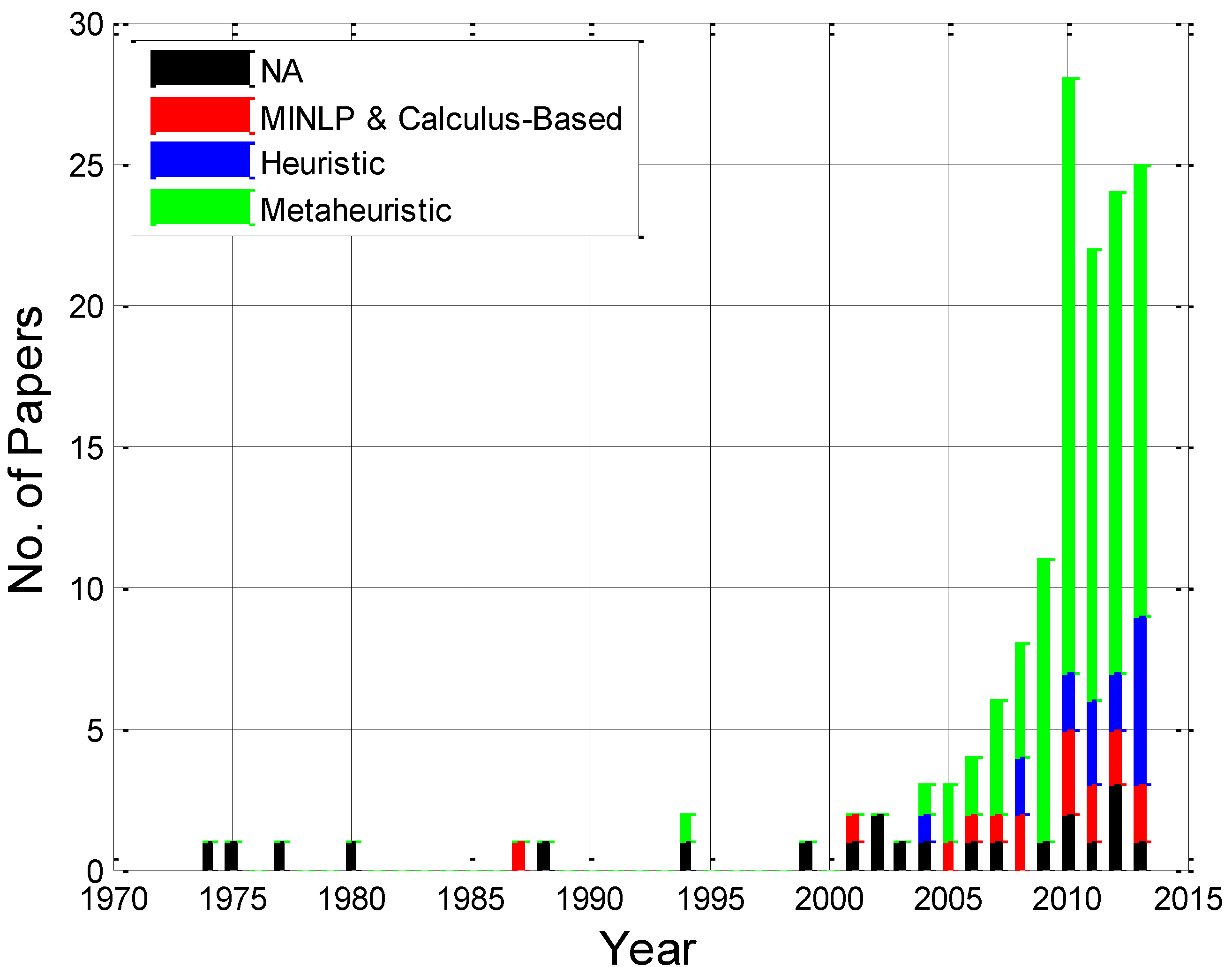
3.3.2. Heuristic Optimization

Since obtaining an optimal solution to the WFDO problem may not be possible with a reasonable amount of computational resources, as pointed out in Section 2.5, or because of the natural limitations of the calculus-based solution procedures, the attention is turned to approaches that compute near-optimal solutions. Essentially, there is an interest to explore the trade-off between the final solution quality and the amount of computational resources spent. While many problems may not have polynomial time solutions, it may indeed be possible to find a solution that is optimal or very close to the optimal. Heuristics (commonly known as approximate algorithms, derivative-free algorithms or black-box methods) are deterministic or non-deterministic solution procedures based on semi-empirical rules that are used to find near-optimal solutions to complex problems. Generally, these approaches are very fast (fast enough to be used in practice), and have improved solutions over traditional calculus-based optimization techniques [140,327]. However, they need to be executed several times to guarantee convergence to a high quality solution. Heuristics do not necessarily require the computation of gradients during optimization and do not necessarily require that the objective function is continuous. Heuristics are classified in two different groups: constructive and iterative. Constructive heuristics build a complete solution by performing multiple sequential deterministic or non-deterministic assemblies of the involved variables while considering all defined constraints (i.e., the value of each variable is decided based on deterministic or non-deterministic rules). Iterative heuristics attempt to improve a complete solution (that can be obtained from a constructive heuristic) by doing a controlled evaluation of the local search space of each of the involved variables. Constructive heuristics are faster than iterative heuristics, but in most cases converge to solutions of unacceptable quality. For highly constrained problems, constructive techniques may even fail to find a feasible solution.

There are several general heuristic frameworks that have been demonstrated to perform well for various types of problems (e.g., the Traveling Salesman Problem (TSP) [333]). Determining which heuristic to use for solving a particular problem is one of the most common (and most difficult to solve) questions in heuristic search. It is common to suspect that some heuristics might perform better than other heuristics when considering a set of different optimization problems, but unfortunately the No Free Lunch Theorems (NFLT) [327,334] suggest that this is not the case. A summary of the NFLT states “for all possible performance measures, no algorithm is better than another when its performance is averaged over all possible optimization problems” [334]. The most basic heuristic search algorithm, Random Search (RS), randomly samples a number of feasible solutions and determines the best solution from the sample. Apparently, any heuristic that evaluates problems more cleverly should always perform better than RS, but as the NFLT suggests, their performance will be the same when averaged over all possible optimization problems. While it may not be possible to perform better than RS over all optimization problems, research has shown that it is possible for heuristics to perform much better than RS for specific problems [335,336,337]. Such heuristics usually take advantage of the structure of the specific problem to obtain near-optimal solutions. This structure may include the constraints of the problem, how a feasible solution is represented (e.g., binary permutation, real-valued string, etc.), or even the instance of the problem at hand. Since any heuristic is equivalent to RS when averaged over all possible optimization problems, any fine-tuning of the driving parameters of the considered heuristic algorithm(s) will inherently create weaknesses with respect to other optimization problems. Therefore, careful tuning of the heuristic driving parameters must be performed when considering a specific optimization framework and should not be based on the suggested values obtained from different optimization frameworks.

Different heuristic strategies have been used to solve the WFDO problem. The first heuristic strategy was provided by Ozturk and Norman [152], who implemented a deterministic greedy constructive algorithm used to solve simplified wind farm scenarios. The reason behind the implementation and use of the heuristic procedure was to overcome the natural complications of the adopted non-linear mathematical model, which, however, showed modest complexity as compared with the models resumed in this work. Greedy heuristics have been retaken recently as shown in the works of Chen et al. [266] and Yin and Wang [265] and have demonstrated the potential to solve complex versions of the WFDO problem. In addition, other approaches in the literature have successfully adopted different heuristics such as the Monte Carlo method [183,187,188,189,238,239], pattern search algorithms [244], viral algorithms [255,256], Powell’s method [257], particle filtering [204], bionic optimization [208], and customized local search algorithms [210,271]. The set of heuristics, however, have never been compared systematically to determine the best performer, thus resulting in an important topic of research.

3.3.3. Metaheuristic Optimization

For some problems, there are known heuristic algorithms which are practically useful, but for many problems the best-known heuristic algorithms have running times too large to be of practical use, despite the fact that they might have polynomial time execution. To overcome this issue, more complex and intelligent heuristics have been developed and are commonly referred as metaheuristics and hyper-heuristics [327]. Metaheuristics are high level procedures designed to find near optimal solutions more efficiently than common heuristics. Hyper-heuristics are higher level procedures designed to find or generate a lower-level procedure that may provide a near-optimal solution to a complex problem. Metaheuristics are commonly based on optimization processes observed in the nature (e.g., Simulated Annealing (SA) [338,339,340,341,342,343,344], Particle Swarm Optimization (PSO) [327,345], Genetic Algorithm (GA) [327,346,347,348], etc.). Some of the multiple remarkable aspects of metaheuristics are that they make only a few assumptions about the function being extremized, they are relatively easy to implement, and do not require the objective function to be continuous or differentiable. Even though, metaheuristics are designed to be problem-independent, some problems that are successfully solved by one metaheuristic algorithm may not be solved when using another metaheuristic algorithm (i.e., metaheuristics are not universal and are subject to the NFLT). In addition, they may require more elementary operations to perform the optimization tasks compared with simple heuristics or calculus-based algorithms. In this regard, the decision of using a metaheuristic algorithm must be based on the problem complexity rather than in its implementation easiness, since for some problems calculus-based algorithms can outperform heuristics and metaheuristics.

Metaheuristics are classified in three different groups: constructive-based, local search-based, and population-based metaheuristics. Constructive metaheuristics are based on a set of heuristics to build a feasible solution. The Greedy Randomized Adaptive Search Procedure (GRASP) [327,349] is considered one of the most powerful constructive metaheuristics and consists of two phases: (1) an iterative procedure made up from a greedy randomized construction (i.e., a semi-greedy heuristic) and (2) a local search iterative procedure, which may be a calculus-based local search procedure or a heuristic/metaheuristic-based local search procedure, that improves the previously constructed solution. Yin and Wang [265] implemented a GRASP algorithm complemented with a Variable Neighborhood Search (VNS) metaheuristic algorithm and showed improved results when comparing them with the results of Mosetti et al. [28] and Grady et al. [232], who employed a genetic algorithm to optimize wind farms under simplified conditions. However, the shortcomings of the proposed GRASP procedure, and other procedures as well, are the need to discretize the search space to define the possible locations of the WTs integrating the wind farm, and the fact that the inclusion of additional variables is not straightforward, requiring a complete reformulation of the state/solution representation.

Local search metaheuristics are based on the fundamental idea in which feasible solutions of similar quality are related. The hope is that if a solution has good quality, then a related solution will also be good (and possible better). The notion of two solutions being related is handled differently in different local search-based algorithms. Local search procedures iteratively modify the value of the design variables, by performing deterministic or non-deterministic actions, resulting in neighbor solutions. The algorithm selects the best neighbor solution at each iteration and repeats the process until no better solutions are found in the neighborhood. The main advantages of local search algorithms are that they are very easy to implement and have few driving parameters. At the same time, they can be very powerful solution procedures for several problems [350,351] including the WFDO problem. The main drawback of local search is that if the search space is too complex (i.e., involving many local extreme points and/or many optimal solutions), the algorithm may not converge to the optimal solution. To overcome this limitation, local search metaheuristics use additional heuristics to decide which is the best neighbor solution (i.e., neighbor solutions with lower quality may be selected).

Different local search procedures have been proposed to solve the WFDO problem. Yin and Wang [265] adopted VNS as a complementary local search procedure to their GRASP implementation, as previously mentioned. VNS was first introduced in 1997 [352] and is quite similar to common local search procedures such as the calculus-based multi-start procedure. VNS performs a local search from multiple neighborhoods and accepts neighbor solutions only if an improvement is made. The difference between the VNS and the multi-start algorithms is that the VNS systematically changes the neighborhoods being explored in two phases: the first phase involves a gradient decent procedure to identify local extreme points, and the second phase involves a random perturbation which allows the algorithm to explore other neighborhoods.

Another successful local-search metaheuristic applied to the WFDO problem is the Simulated Annealing (SA) algorithm [327,338]. SA is based on the process of annealing of solids, which is a thermal process for obtaining low energy states in solids by exposing them to a heat bath. The annealing process consists of the following two steps [343]: (1) increase the temperature of the heat bath until the solid melts; and (2) slowly decrease the temperature of the heat bath until the particles arrange themselves in the low energy ground state of the solid. In the melt phase, the constituent particles arrange themselves randomly, and in the cooling stage the particles arrange themselves in an organized lattice. The analogy between the annealing process and the optimization process is that potential solutions of the studied problem are comparable to states of a physical system undergoing a process of annealing, and the quality of a potential solution is equivalent to the energy of a state [338]. While local search (and variable local search) generally will accept transitions between neighbor solutions only if its quality is better than the current solution, SA has the capacity of allow transitions between solutions whose qualities are worse than the current solution in the hope of avoiding getting stuck in a local extreme point. The transition to a worst solution is modeled as a probabilistic process, which relies on the Metropolis criterion [327], and depends on the actual state and the new state quality. The probability of rejection of states with lower quality increase as the search continues (i.e., SA behaves as a greedy algorithm), thus simulating the arrangement of particles in an organized lattice during the cooling process. The SA’s ease of implementation, convergence properties, and ability to escape local extreme points have made it a popular technique during the past two decades. The SA-based metaheuristic has been implemented to solve different versions of the WFDO problem showing better or equal performance than other metaheuristics such as the genetic algorithm [154,156].

Population-based metaheuristics encompass all solution procedures that use multiple agents or individuals (i.e., potential solutions), which are interacted between them, to trace out for better individuals. Population-based algorithms rely on the idea in which the best characteristics of the best individuals can be combined to produce a better individual. The Genetic Algorithm (GA) is the most used population-based metaheuristic in the WFDO problem [56,134,135,156,159,160,161,163,165,199,200,207,235,237,245,250,254,278,301,307,353,354,355,356,357]. The GA [327,346] refers to a class of adaptive search procedures based on the principles derived from natural evolution and genetics. In the GA, genes represent the design variables, and potential solutions (i.e., individuals) are represented by chromosomes. Like other methods, as the GA proceeds through generations (i.e., iterations), it holds a set of possible solutions referred to as the population. Based on the fitness value (i.e., the quality of a solution), which is determined through the evaluation of the population’s individuals, two individuals (i.e., the parents) are selected and are combined through genetic operators (crossover and mutation) resulting in two new individuals (e.g., the offspring). Many different variants of genetic algorithms have been considered in the literature [327] differing in the way genetic operators act over the population and the way individuals are represented. Research has demonstrated that the performance of a genetic algorithm relies upon the proper choice of the selection and crossover mechanisms and the proper design of the individual representation.

Another successful population-based metaheuristic algorithm applied to the WFDO problem is the Particle Swarm Optimization (PSO) algorithm [184,192,193,201,203,212,243,264,269,353], which was developed by Eberhart and Kennedy in 1995 [345]. The PSO algorithm is inspired by the social behavior of fish schooling and bird flocking. The PSO algorithm relies on the idea in which different paths having different length and complexity can lead to an optimal solution (i.e., different particles, or individuals that represent a possible solutions, can take different paths that lead to the same destination, which is assumed to be the place where the performance metric is the best). The PSO algorithm tracks the best position and velocity of each particle integrating the swarm and updates both quantities iteratively. The particles will move in the search space until the stopping criteria is met, which is established when the optimal location has been determined or a given number of iterations have been performed.

A very detailed study that contrasts the different SA, GA and PSO implementations used in the WFDO problem is given in [154]. Additional solution procedures based on Ant Colony Optimization [195] and Neural Networks [262] have been used to solve different versions of the WFDO problem. All approaches have shown promising results. However, these solution procedures have been implemented in different scenarios having variable complexity, unknown optimal solutions, substantial differences in main objectives and model constraints, thus limiting any objective conclusion of their effectiveness while solving the WFDO problem. In this regard, a systematic evaluation of solution procedures in realistic wind farm scenarios will provide a basis for the judgment of the performance of each solution procedure in the solution of the WFDO problem. In addition, the performance evaluation of additional heuristics and metaheuristics based on the TABU search, scatter search, memetic algorithms, cuckoo search, etc. has not yet been performed.

3.3.4. Multi-Step, Nesting and Hybridization

New strategies have been developed to handle complex problems, which may contain embedded optimization problems. The most basic strategy is the multi-step optimization, which consists of computing a solution to the problem by first using one type of optimization procedure. The solution is later given as an input to a second optimization procedure, which in turn aims to improve the quality of the given solution. The process can be repeated systematically by using the same optimization procedures or by including additional optimization procedures. Multi-step procedures are commonly used to handle the limitations of certain algorithms (e.g., algorithms that need the discretization of the search space) by systematically using another algorithm(s) that has different limitations. If the problem contains embedded optimization problems, then the common procedure is to obtain the best solution to the general problem to later give it as an input to the embedded optimization problems (e.g., in the WFDO problem, the first step may be to determine the best wind farm layout to later optimize the design of the inner electrical infrastructure layout; this procedure, whoever, may compromise the financial balance of the project). The multi-step procedure has been adopted in the solution of the WFDO problem several times. In the multi-fidelity approach (i.e., approaches that systematically increase the complexity of the problem being treated) proposed by of Réthoré et al. [166], within the TOPFARM framework, the first multi-fidelity level can be categorized as a multi-step procedure, in which the solution of a Simple Genetic Algorithm (SGA) is given as an input to a Sequential Linear Programming (SLP) algorithm. It must be noted that higher levels in the proposed multi-fidelity approach consider the inclusion of advanced objective functions and sub-models and, therefore, cannot be categorized as multi-step procedures. In addition, it should be noted that some metaheuristic algorithms, such as GRASP [265], include multi-step procedures as a part of their optimization strategies. González et al. [277], within the scope of the WFDO problem, demonstrated that sequential multi-step procedures do not lead to the optimal solutions of problems having embedded optimization problems, instead of global procedures (or nested procedures) that take into account all the design variables at once.

Solution procedures using the concept of nesting include different algorithms in sub-levels during the overall optimization. The difference with the multi-step approach is that in the nesting approach a combination of two or more algorithms, usually a population-based metaheuristic and a local search algorithm, are used sequentially through the iterative process. The optimization of the design variables is performed first by the leading algorithm (e.g., population-based metaheuristic) and then, in the same iteration, the nested algorithm(s) improve the solution quality by performing additional modifications to the design variables. The nesting approach, as suggested by González et al. [277], might lead to improved solutions in contrast with muti-step approaches.

Hybridization [327,358,359,360] procedures are commonly associated with nesting procedures. However, in a strict sense, hybridization refers to the development of a new method that combines the best characteristics of other individual methods. Thus, the hybrid method is expected to have superior performance when contrasting with the performance of the individual methods composing the hybrid method. Hybrid methods are hardly found in the literature and are generally classified as new algorithms.

4. Research Needs and Trends in Wind Farm Design and Optimization

The general research trend in WFDO is focused on balancing the trade-off between the development of complex sub-models (by gradually including additional adverse factors and variables) and the inherently complexity added to the problem. Although computational technologies are being improved quickly, they are generally the limiting factor for the treatment of the WFDO problem. Thus, researchers and wind farm designers rely on advanced solution procedures such as metaheuristics to tackle the problem. In addition, researchers rely on additional concepts that help setting the optimization framework such as the preprocessing and the multi-fidelity procedures. The concept of preprocessing, within the WFDO problem scope, refers to a set of computations performed to build a wind farm scenario, previous to the optimization procedure. Preprocessing includes the definition of the local wind field (e.g., through the use of CFD techniques), pre-convolution of WT power curves, pre-calculation of individual loading cases for WT components using aero-elastic simulations, construction of databases having relevant information (e.g., WT characteristics such as maximum height, minimum height or costs), etc. Preprocessed data can be interpolated during the optimization procedure, thus significantly improving computational times. However, preprocessing techniques typically require additional assumptions (e.g., conventional CFD techniques used to estimate the local wind resource assume steady state conditions) and depend on the accuracy of the interpolation procedure. Preprocessing techniques can be combined with other relevant techniques such as the multi-fidelity approaches in which the complexity of a problem is gradually increased during the optimization procedure. As proposed in the novel work of Réthoré et al. [166], the concept of multi-fidelity can significantly improve computational times and solution quality. However, both the preprocessing and multi-fidelity approaches have been scarcely applied to the WFDO problem, thus denoting an important area of research.

New issues regarding the potential conflict of interests (e.g., effects of the presence of nearby projects that are not necessarily wind farms) and the design of multiple wind farms under uncertain conditions have been treated recently [171,308] and are recognized as potential problems that will be more frequent in the near future. However, due to the different scales of such problems, certain assumptions and models (e.g., wind field modeling and wake modeling) may not hold and will require additional research to determine its validity and/or its extension.

Another important area of research in WFDO focuses on the validation of the various sub-models described in Section 3.2. In addition, the complete validation of the outputs of the WFDO procedures remains a complex problem to solve. The specific research trends on the performance metrics, sub-models and solution methods are discussed in the next sub-sections.

4.1. Performance Metrics

Previous research works [135,199] have demonstrated that the outputs of the WFDO process are highly sensitive to the choice of the objective function (i.e., there is high dependency of the best wind farm layout on chosen performance metric). However, a complete sensitivity analysis describing the effects of using different performance metrics and including different adverse factors during the optimization procedures has not yet been performed. In addition, a complete sensitivity analysis of the resultant optimized layouts considering different atmospheric conditions (e.g., for a wide range of inflow conditions and different thermal stratification conditions) has not yet been performed.

The general trend of the optimized results obtained among the different approaches adopted in the literature is to install few and large capacity WTs, in contrast to installing many small capacity WTs, in irregular arrays in which wake effects are minimized. An interesting trend observed in all the reviewed works, without regard to the chosen objective metric and optimization procedure, is that significant improvements (in terms of the selected performance metric) can be obtained due to the application of systematic optimization methods over micro-siting methods based on rules-of-thumb.

The energy yield alone has proven not to be the best objective function for practical purposes, since the net economic benefits obtained from the wind farm may not always increase monotonically with increasing converted energy. This is mainly due to the effects of wakes and turbulence on the power conversion and loading and/or by the required costs for the acquisition of WTs and the construction of civil engineering and electrical infrastructure. Therefore, the wind farm with the largest energy conversion does not necessarily have to be the one that produces the best economic profits. The need for all-encompassing design variables requires the costs to be computed besides the energy conversion yield. However, significant improvements in the traditional way to calculate the annual energy production of wind farms (that may include the inclusion robust multivariate probability density functions and the inclusion of additional factors such as turbulence, wind shear or WT dynamic loading) are required in order to improve the energy yield predictions and lower the impacts of risk and uncertainty on the expected economic returns.

The most suitable performance metrics are the NPV and the FB, since the wind farm purpose is to produce the largest possible economic profit. The CoE alone cannot provide conclusions about the viability of a particular project, thus it should be incorporated as a complementary economic metric. The inclusion of additional finance metrics such as benefit cost ratio (the present value of all benefits divided by the present value of all costs), the internal rate of return (IRR, is the value of the discount rate that gives a NPV of zero), and discounted value indicators such as the payback period (the capital cost of the project divided by the annual average return) might improve the understanding of the absolute financial prospections in the WFDO problem and will include the possibility of performing additional analysis that might be necessary when considering different energy markets. In this regard, the inclusion of dynamic models for energy price setting and the integration of regulation models for energy marketing remain complex problems yet to be solved.

4.2. Sub-Modeling of Adverse Factors

A wide range of varying conclusions about the different effects of the adverse factors, described in Section 2.2, produce in the resultant optimized wind farms were provided in the literature. However, most of the conclusions are based on sub-models in which the effects of such factors were limited or oversimplified. In addition, the conclusions are commonly based on contrasts between pairs of factors that are usually in conflict. Only a few works were able to address the overall effects of including different factors [54,55,56,199,234,278,310]. Two general kinds of effects in the resultant wind farm layouts were observed; some factors (e.g., infrastructure costs) induce pressure to concentrate WTs in high dense irregular clusters within the wind farm area while other factors (e.g., wake effects, turbulence and noise) induce pressure to separate WTs. Both trends affect the optimal number of WTs and the wind farm size. These observed trends, however, are highly dependent on the chosen performance metric and further analyses are required to understand which factors, and under which conditions, dominate during the WFDO process. In addition, the inaccuracies and validity ranges of the common used sub-models may be influencing the shape of the obtained near-optimal solutions, thus the validation and extension of sub-models is considered the most important aspect to be improved in the development of the WFDO problem. Some of the most important modeling limitations are described next:

Sub-models describing the impacts of WT wakes are limited, since crude assumptions about the wake expansion, wake merging, wake rotation, partial wake operation, wake meandering and 2-way interactions with large scale turbulence structures are commonly considered.

State-of-the-art sub-models describing the structural degradation costs of the different WT members and the costs associated to O&M are still not validated, and rely on aero-elastic codes that simulate the loads that each component will undergo while operating, as described in Section 3.2.2 and Section 3.2.6. Although the quantification of WT structural degradation is a complex task that depends on the local climatology, the particular WT design, and its operation, it is expected that some WT members (e.g., gear box, main shaft, and WT blades among others) will be more affected than others while operating. Thus, significant research is required to identify which components are the most affected, and under what conditions, and to improve the cost prediction of their degradation.

The civil infrastructure cost models are significantly different comparing onshore and offshore wind farms as described in Section 3.2.3 and Section 3.2.6. State-of-the-art infrastructure cost models for offshore wind farms consider all relevant factors during the design of the WT substructures and foundations (e.g., seabed depth, tower mass as a function of wind and wave loads among others). However, current existing models for onshore projects consider that foundation costs are proportional to the land bearing capacity. The inclusion of additional variables such as the expected WT loading and the type and capacity of the WT foundation might improve the civil infrastructure modeling in onshore sites. The most comprehensive civil and electrical infrastructure cost models are highly sensitive to time variations of the price of their constituent components. In addition, an important lack of modeled physics in power transmission was observed, which in turn affect the predictions of the effective expected electric energy conversion. An adequate combination of improved models describing electrical infrastructure costs, electrical losses, electrical components capacity and reliability is required.

An important aspect that has been largely neglected is the topography of the wind farm area. The topography does not only affect the computation of the local wind field but also affects the development of other adverse factors such as noise, wakes, turbulence and electromagnetic fields. Literature works commonly consider a flat square area and assume, with the exception of a few works [55,219], that the wind field characteristics are identical throughout the entire site. A flat square area assumption certainly holds for offshore sites, but it is very unrealistic for onshore sites, where terrain is rarely flat, has non-uniform roughness and irregular boundaries. The reason behind ignoring the topography complexity is due to the fact that it is hard to obtain reliable estimations of its effects though simple models and cheap computational routines. Thus, additional assumptions are commonly considered when optimizing onshore wind farms (e.g., it is commonly assumed that WT wakes follow the terrain shape and are not affected by the presence of the ground). However, as previously mentioned, the use of commercial software (see Section 4.4) and the concept of preprocessing might help to overcome some of these limitations. Therefore, the description of how wakes, turbulence, noise and electromagnetic fields evolve in the domain while considering the local topography remains an important problem to address. In addition, common approaches in the literature neglect the effects of topography in the design of the civil engineering and electrical infrastructure. In complex terrain, the total length (and therefore the total cost) of the auxiliary roads or the MVAC collection lines can be significantly different from that for flat sites. This fact limits the applicability of the traditional Euclidean minimum spanning tree and the Steiner tree approaches and induces the necessity for the development of new robust approaches.

The uncertainty and risk modeling of wind farms has been scarcely treated in the scope of the WFDO problem as pointed out in Section 3.2.5. Two important unaddressed problems in the topic have been identified: (1) only a small set of factors that contribute to the overall uncertainty were included in the optimization frameworks of the literature works; (2) The treatment of uncertainty is based on the assumption in which the stochastic variation of certain variables can be described using predefined statistical distributions. The assumptions, however, are not validated and require additional research.

Environmental and/or social impacts within the WFDO procedures have been neglected in most works as pointed out in Section 3.2.4. Although their inclusion into an optimization framework demands significant efforts in both the modeling and optimization stages, they should not be discarded as they usually influence the viability of wind projects.

4.3. Solution Methods

The general research trend in the solution methods for the generalized WFDO problem is focused on balancing the trade-off between the obtained solution quality and the computational requirements. Hence, the adoption of metaheuristic algorithms in integrated schemes, while employing the concepts of multistep, nesting and hybrid optimization is necessary to tackle the problem. Investigation related to the adequate comparison of solution procedures in realistic wind farm scenarios, and while employing the same state-of-the-art performance metrics and sub-models is required. This is due to the fact that certain comparisons between different solution procedures, that are reported in the literature are meaningless [241,242], since the adopted performance metrics were different or the amount and type of contrasted algorithms were limited. In addition, the evaluation of other optimization algorithms that have not been used to attempt solve the WFDO problem may provide a wider and more objective perspective about which type of algorithms perform best.

Another important aspect to consider is that some solution procedures rely on the relaxation of the complexity of the problem (i.e., relaxation of the model or variables complexity). While this may provide interesting conclusions about the mathematical behavior of the problem, relaxations over already simplified models can lead to important inaccuracies, which in turn impact not only the expected wind farm performance but also the solution shape of the problem. Therefore, the proposed solution procedures must tackle the problem without affecting both the mathematical form of the model and the design variables. Many solution procedures, such as the ones based on the Genetic Algorithm, require the discretization of the wind farm site, thus limiting the available locations where WTs can be erected, which in turn impacts the solution quality of the problem as demonstrated in [242,259]. Although it has been suggested to use irregular, finer and non-uniform discretization grids to improve these limitations [242], the selection of the type, size and refinement of the grid is equally hard as selecting the WT individual locations over a continuous space, thus denoting an important area of improvement for such solution procedures. In addition, most of the optimization procedures reported in the literature have assumed a constant number of WTs or a maximum number of WTs, justified by the assumed limited investment capacity of the wind farm designer. The assumption, however, is very unrealistic, since the financial resources on the worldwide market are very large. In practice, what limits the size of a wind farm (in terms of installed capacity) are practical considerations, such as the maximum amount of energy that can be sold off in an offtake agreement, the limited site space, and very often the transmission capacity. Other approaches, in which the discretization of the wind farm site is considered, have linked the fixed available WT locations with the number of WTs, thus reducing the number of design variables with the implication of restricting the possible wind farm layouts and thus the solution quality of the problem, as previously discussed. The determination of the optimal number of WTs, assuming no predefined investment capacity or any linkage to the process of domain discretization, is complex and the best procedures perform a sensitivity analysis to determine its optimum value. However, sensitivity analyses may require long computation times and will depend on the effectiveness of the solution procedure to find optimal or near-optimal solutions for scenarios having different predefined number of WTs. It should be noted that optimized wind farm layouts having different amount of WTs can be significantly different, thus hindering the determination of the optimal number of WTs based on solutions to scenarios having different number of WTs. In this regard, the development of adaptive algorithms that include the number of WTs as a design variable is required.

Most of the studied wind farm scenarios assumed a square boundary. The reason behind this trend is related to the ability of the proposed solution procedures to handle restrictions. As the boundary shape complexity is increased, the complexity of the wind farm model constraints increase, thus affecting the performance of the proposed solution procedures. In order to deal with this issue, a novel multi-boundary constraint model, which is based on the optimal design of polygonal geometries used to approximate the shape of complex boundaries, and the incorporation of a ray intersection method, used to determine if WTs are located on feasible locations, was recently developed by Gu and Wang [361]. The robust model of Gu and Wang may be successfully implemented in different optimization frameworks, thus enhancing the constraints management.

The solution procedures proposed in the literature have been able to find better solutions than the ones proposed by Mosetti et al. [28], traditional rules-of-thumb (e.g., equally spaced or grid-like siting schemes) and initial random solutions, but none of them have been able to assess the quality of the solution found (i.e., no upper bound of the objective value, with the exception of the objective value if no wake effects are taken into account, has been provided). Therefore, it is inadequate to assume that the proposed algorithms reached optimal solutions without knowing the shape and the objective value of optimal solution. As discussed in Section 2.5, optimal solutions of the WFDO problem can be verified only for small instances, and further comparisons between solution procedures, assuming larger scenarios, can be performed only in a relative basis, if no other information is available or can be inferred about the optimal solution.

None of the reviewed works discussed how the algorithm-driving parameters were tuned. A poor tuning process can significantly affect the performance of the tested algorithms, as discussed in Section 3.3.2. In addition, none of the authors of the reviewed works reported the average efficiency of the tested algorithm. It is well known that heuristic and metaheuristic algorithms require several executions to reach near-optimal solutions. In this regard, statistical design of experiments could provide useful information to determine the average efficiency of the tested solution procedures and to determine the best value of the algorithm-driving parameters.

The complexity of the WFDO problem requires a multi-objective framework, in which the evaluation of the performance metric(s) and all adverse factors can be performed systematically. The obvious limitation of such framework is the natural non-parallelizable characteristics of the problem, which in turn imply that a significant amount of time will be required to evaluate potential solutions throughout the optimization procedure. However, detailed research on the performance improvements of incorporating parallelism on the embedded optimization problems, such as the civil engineering and infrastructure design, are yet to be performed.

4.4. Commercial Software

Software tools are now being used to optimize wind farms. The most widely used commercial programs, including its strategies, are presented next.

The Wind Atlas Analysis and Application Program (WAsP) v11 [48], developed in 1987 by the RISØ National Laboratory, is considered the industry standard software for wind resource assessment and wind farm micro-siting. The software includes two different approaches for the wind resource quantification and wind resource mapping. The first approach is based on the so-called Wind Atlas methodology, which in turn is based on a set of linearized flow equations and is suitable for sites showing modest terrain complexity and near uniform roughness conditions. The second approach is based on the Reynolds-Averaged Navier-Stokes equations complemented with a standard k–ε turbulence model, which is suitable to be used in complex terrain. Both approaches perform the procedures described in Section 2.1 to obtain accurate estimations of the local wind field and rely heavily on the quality and quantity of the measured data at the site. The WAsP software includes the possibility to perform different types of analysis regarding the wind farm production, the wind farm efficiency (incorporating the Park model, which is based on the Jensen-Katic wake model), wind data analysis, wind climate estimation, and wind atlas generation. However, it lacks an optimization framework for automated micro-siting. Nonetheless, upcoming versions of WAsP will incorporate the TOPFARM framework [164,165,166,306,354] as a complementary module that will allow to perform systematic optimization of wind farms.

WindPRO v2.9 [49] is a robust tool developed by EMD International A/S that incorporates the WAsP engine for wind resource quantification. WindPro includes several different modules for the simulation and quantification of the wind farm energy production (incorporating the WAsP Park model to determine wake-based and turbulence-based energy losses) and environmental impacts (including noise impact, shadow flicker, and visual impacts). In addition, it includes modules for the electrical layout design and its optimization (including the quantification of power losses) and a robust financial balance model. WindPro optimizes the wind farm layout using the annual energy production as a performance metric while accounting for noise thresholds. However, shadow flicker, visual impacts and financial prospections are not accounted during the optimization procedure. The optimization is based on a pre-calculated wind resource map made up from the WAsP engine, which accounts for both the topography- and the roughness-based induced effects. Different types of optimization processes, based on greedy heuristics, can be performed: (1) a stochastic and gradual addition of WTs into the wind farm (without changing the preexisting WT positions) until no more WTs can be placed or a predefined maximum number of WTs is reached; (2) an iterative modification of the wind farm layout (by changing WT separation distances assuming a staggered or grid-like siting scheme); (3) an iterative filling up of the available land with WTs, resulting in a high dense WT cluster; or (4) optimization of noise operation modes for fixed wind farm layouts. The optimization processes depend on a set of predefined parameters such as the minimum distance between WTs, a predefined installed capacity per unit area and predefined restricted zones.

The WindFarmer v5.2 [50] tool, developed by DNV-GL Garrad Hassan, is similar to WindPro, as it incorporates the WAsP engine for wind resource quantification and offers a set of different modules for the design and optimization of wind farms. It includes the possibility of perform analysis regarding the energy production, noise impacts, visual impacts, shadow flicker, turbulence effects, electric system design, uncertainty modeling and financial balance prospections. Wake losses are calculated with the use of the DNV GL’s CFD model, which is based on the Reynolds-Averaged Navier-Stokes equations complemented with an eddy viscosity turbulence closure. The optimization procedures are based on greedy heuristics, which can either maximize the annual energy production or the financial balance of the project. The software includes the possibility of adding a customized financial model and actively updates the selected performance metric during the optimization process. The optimization process includes environmental impacts (noise, visual impact, shadow flicker and turbulence intensity) as constraints with predefined thresholds.

Meteodyn WT v4 [51] is a CFD-based tool for wind resource assessment and wind farm design. The wind flow modeling approach is based on the Reynolds-Averaged Navier-Stokes equations, which are complemented with a one-equation turbulence model (i.e., the turbulent kinetic energy equation). The software is able to assess the annual energy production of the wind farm while accounting for wake effects (which are modeled using the Jensen-Katic wake model). However, it currently lacks an optimization framework for automated micro-siting as well as of additional modules to perform environmental impact and uncertainty assessments.

Wind Farm v4.2 [52] is a general tool, made by ReSoft, for the analysis, design and optimization of wind farms. The software is capable of performing wind resource assessments based on the linearized steady-state flow model MS-Micro/3 (having the same technical background as WAsP), developed by the Atmospheric Environment Service of Environment Canada and Zephyr, and predict long term variations in wind speed using the Measure-Correlate-Predict (MCP) method. The wind farm energy yield is estimated based on pre-constructed wind maps while accounting for wake losses, which are modeled using different wake models including the Ainslie and the WAsP Park models, and includes additional losses caused by turbulence. Similarly to WindFarmer and WindPro, Wind Farm is capable of performing noise estimations (based on the ISO 9613 standard [315]), as well as visual and shadow flicker assessments. The optimization module of WindFarm determines the optimum layout of WTs based on a pre-defined set of constraints such as the WT minimum separation, separation from houses, noise level and ground slope. The performance metric can be either the ${\text{AEP}}_{\text{Farm}}$ or the CoE (considering a simple form of the capital costs as the value to be minimized) of the wind farm. The optimization strategy is based on a greedy local search heuristic. The optimization process is repeatedly restated in order to avoid local minima or maxima. At each restart, each turbine might be moved randomly within a specified movement limit, which is reduced by a specified step size on each restart until the movement limit is reduced to zero.

WindSim v6.2 [47] is a CFD-based tool for wind resource assessment and wind farm design and optimization. The wind flow modeling approach is based on the Reynolds-Averaged Navier-Stokes equations, which are complemented with different kind of turbulence models (e.g., standard k–ε, RNG k–ε and the standard k–ω). The wind farm energy yield is estimated based on pre-constructed wind maps while accounting for wake losses (which can be quantified using different wake models such as the Jensen-Katic [23], Larsen [25] or the Ishihara [288] models). The objective performance metric of the proposed optimization framework is the Net Present Value (NPV) of the project. The optimization procedure aims to define the best location of a predefined number of WTs while accounting for multiple restrictions such as the minimum distance between WTs, terrain inclination, flow inclination, effective turbulence intensity (which is estimated from both the measured turbulence intensity at the wind farm site and the simulated turbulent kinetic energy), wind shear, and extreme winds (which are estimated by the method of Independent Storms) [362]. The optimization process is repeated while varying the number of WTs (N) in the range $1\le N\le N_{max}$, where N_max is a predefined maximum number of WTs. The output of the overall optimization process is a concave curve describing the NPV variation of the project as a function of the number of installed WTs, which in turn define the best number of WTs and the best layout design. Two different algorithms may be selected to perform the optimization task; the local search Simulated Annealing metaheuristic algorithm, which may or may not take into account wake effects, modeled by the Jensen–Katic model, during the optimization process; or a local search calculus-based algorithm that optimizes the wind farm layout while considering a relaxed mixed integer nonlinear model. The optimization process ignores the civil engineering and electrical layout design and any other environmental impacts during the optimization process.

AWS Truepower OpenWind^® Enterprise [46,363] software is a general GIS tool for wind resource assessment (based on a mass-conservation wind flow model) and wind farm micro-siting optimization (which include both wake and turbulence effects in energy conversion, which are modeled using different engineering wake and turbulence models). OpenWind^® implements either the ${\text{AEP}}_{\text{Farm}}$ or the CoE as objective performance metric during the wind farm micro-siting optimization, in which the decision variables are the number and position of WTs and the civil engineering (auxiliary roads) and the electrical infrastructure layout design, while considering existing infrastructure and multiple physical constraints. The software includes the possibility of performing shadow flicker, visual impact, noise impact (based on the ISO 9613 [315]), uncertainty and control (e.g., WT scheduling) assessments. Such assessments, however, are not considered during the optimization process. OpenWind’s solution procedure is based on an iterative non-deterministic greedy heuristic algorithm, in which the WT coordinates are modified by random Gaussian-distributed perturbations. The number of WTs is updated iteratively depending on predefined WT capacity factor thresholds. A set of different heuristic rules are adopted to obtain feasible solutions during the optimization process (i.e., a set of restrictions are given to the program, which in turn define feasible zones in which WTs can be located).

4.5. Misconceptions

Several misconceptions that have been propagating in the literature were identified and are summarized next:

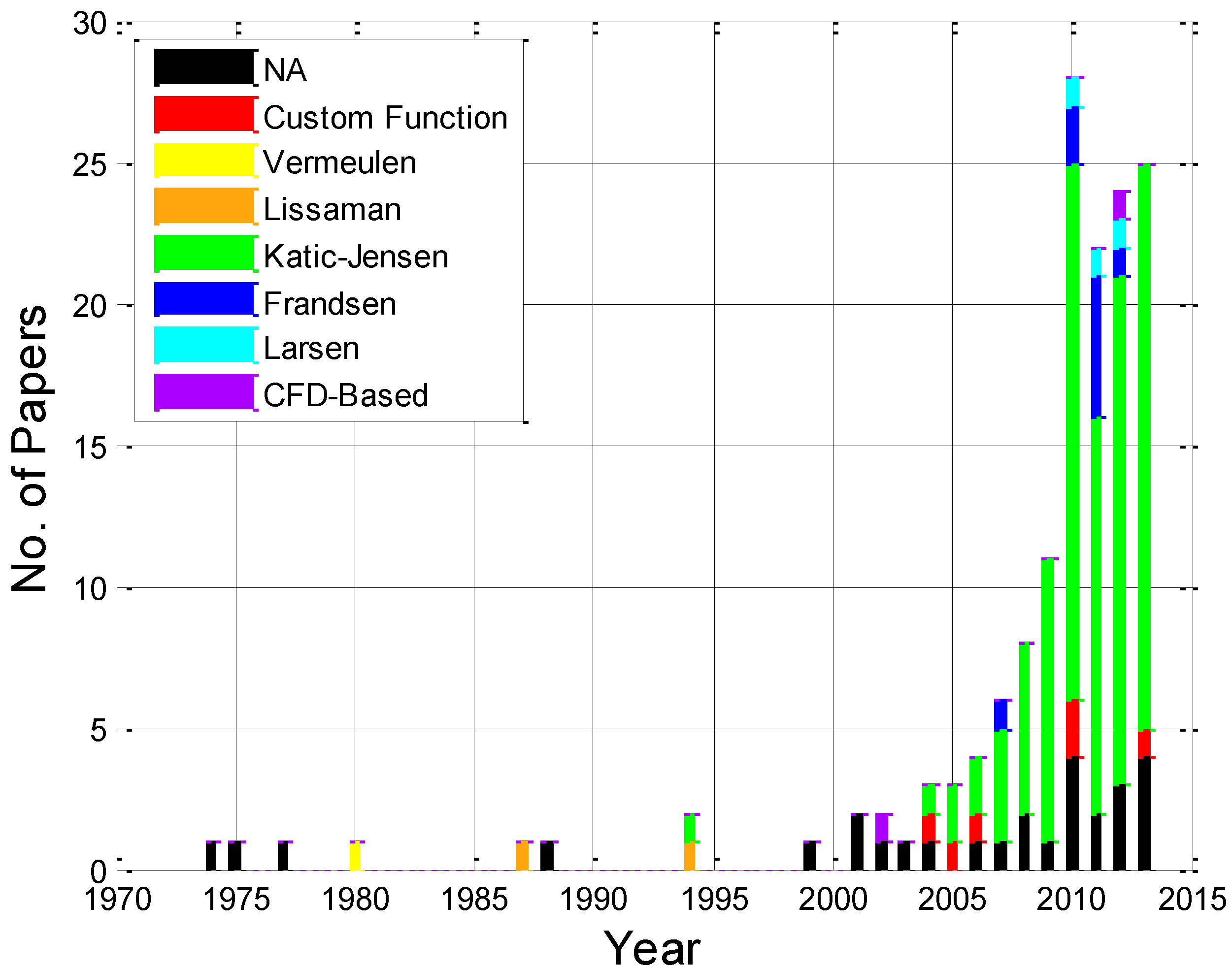
• Different denominations have been arbitrarily given to the engineering wake models (e.g., wind farm models, flow models and linear flow models) and have been used indistinctly through the literature. Generally, wind farm models refers to holistic models that take into account not only wake effects but other factors such as the ones described in Section 2.2 as well. Flow models are commonly referred to as models based on the fundamental laws of fluid mechanics, which quantify the fluid-fluid or fluid-structure interactions. Although wake models may quantify the interactions between different layers of a fluid flow, they are less fundamental than the laws of fluid mechanics. Thus, clear distinctions must be provided to avoid generating confusion. The Jensen-Katic wake model is commonly referred to as a linear wake model. This denomination is given since the wake expansion is assumed to be a linear function of downwind distance from the WT. This, however, introduces a misleading concept about the mathematical complexity of the model. The Jensen-Katic wake model is a non-linear model, Equation (39), that quantifies the wind speed evolution of the wake of WT.
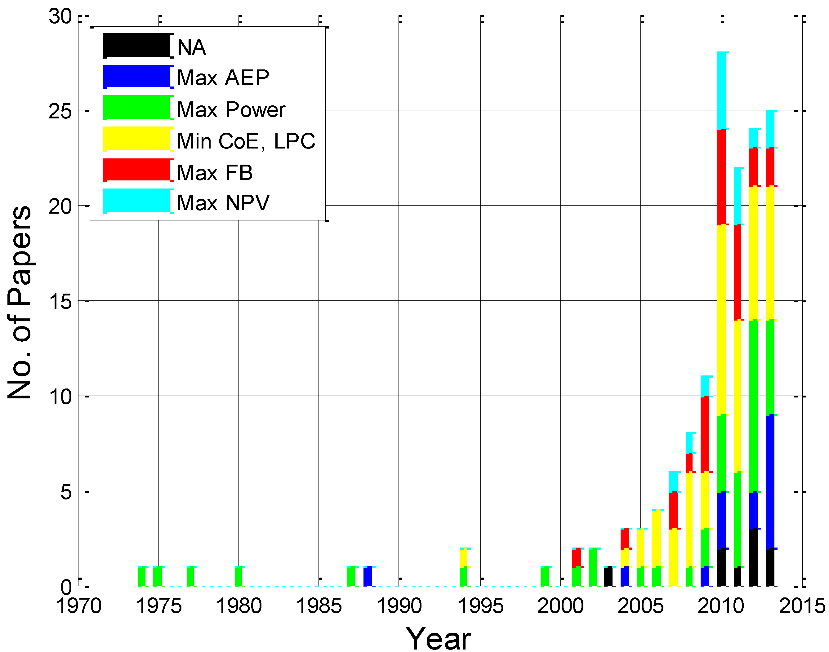
• Different performance metrics were adopted in the literature, including “the cost of power” [28,232]. As pointed out by Tesauro et al. [169], the denomination “cost per KW of power produced” contains two logical errors. (1) The total cost of a wind farm, composed of fixed and variable costs, is commonly calculated on a 20-year baseline and is therefore based on integral quantity, while the wind farm power [kW], defined as the energy converted per unit of time, is a differential quantity by nature. The ratio between the two is meaningless. The Annual Energy Production (AEP) on the contrary, is defined as the integral of power over a period of one year and is measured in [kWh/y]. Thus, the ratio of the wind farm total costs and the AEP (i.e., the cost per kWh of energy) and has an adequate physical meaning and is referred as the Cost of Energy; (2) The denomination “power production of the wind farm” is against the first law of thermodynamics, since energy cannot be produced or created, thus and adequate denomination would be “the power conversion of the wind farm”.
• A linear combination of objective functions, involving different type of variables, is numerically possible but is inadequate due to misleading dimensioning. Examples of linear combination of performance metrics are given in [28,239].
• The computational complexity theory aims to classify problems according to their type and complexity. Although optimization problems are the most treated problems in the literature, other different kind of problems exist such as functional problems or decision problems. Functional problems are problems that produce an output for every given input. Both the type of inputs and outputs can be significantly different, including real or integer numbers, strings, or even abstract objects. Decision problems are problems that return a Boolean answer for a given set of input parameters. Depending on the type of problem treated and its time or space complexity, different complexity denominations are given. Decision problems that can be evaluated by a non-deterministic Turing machine in polynomial time are referred as problems with NP complexity. Optimization problems that can be evaluated by a non-deterministic Turing machine in polynomial time are referred as problems with NPO complexity. Functional problems that can be evaluated by a non-deterministic Turing machine in polynomial time are referred as problems with FNP complexity. In the literature, it is common to find inadequate complexity denominations (e.g., the WFDO problem has been referred as an NP-hard optimization problem [56,152,153,154]), which in turn are commonly based on subjective reasoning rather than in formal demonstrations based on suitable reduction methods, as described in Section 2.5.

5. Conclusions

This work presented an exhaustive survey of the state of the art in the wind farm design and optimization problem. After almost four decades of research, a significant amount of contributions of variable complexity has been reported in the literature, which have enhanced both the understanding of the physical process of wind energy conversion and the techno-economical modeling of wind farms. This topic is currently gaining popularity in the industry, because of the potential economic improvements it offers. However, the applicability of the proposed optimization frameworks in the design of real wind farm projects is currently limited by the modeling complexity of the different physical processes involved during the wind energy conversion, by the current optimization strategies, and by the available computational resources. In addition, the slow inclusion of physics and the use of idealistic scenarios to perform comparisons between different implementations is limiting the applicability of the developed approaches in the design of real wind farms.

The most important research trend in the WFDO problem is focused on improving the formulations describing the expected energy conversion of the wind farm, the WT wakes and turbulence impacts, the WT structural fatigue and degradation, the various types of environmental impacts, the overall electric system losses and reliability, and the uncertainty and risk management. New holistic models are required to improve the wind farm performance modeling and its optimization. In addition, optimization frameworks must encompass all the design variables during the micro-siting process, since current existing approaches have limited the number of design variables and their degrees of freedom, thus significantly affecting the potential benefits. The specific research agenda in WFDO is summarized next:

-

Inclusion of all state-of-the-art sub-models, describing all the adverse factors, and design variables in an all-encompassing procedure.

-

Sensitivity analysis of the effects the selection of different objective performance metrics produce in the resultant optimized wind farms.

-

Sensitivity analysis of the effects that each adverse factor produces in the optimized wind farms, while considering realistic scenarios.

-

Systematic evaluation of different solution procedures, each solution procedure being fine-tuned.

-

Investigation of the effects the different uncertainties produce in the optimized wind farms.

-

Improvement of sub-models, following the observations given in Section 4.

-

Inclusion of control aspects, systematic optimization of multiple wind farms and modeling of the effects of potential conflict of interests.

References

1. Global Wind Statistics 2012; Global Wind Energy Council (GWEC): Brussels, Belgium, 2013; pp. 1–4.
2. Global Wind Report 2012; Global Wind Energy Council (GWEC): Brussels, Belgium, 2013; pp. 1–72.
3. AWEA Wind Industry Market Reports for 2013; American Wind Energy Association (EWEA): Washington, DC, USA, 2013.
4. Templin, R.J. An Estimate of the Interaction of Windmills in Widespread Arrays; Laboratory Report LTR-LA-171; National Aeronautical Establishment: Ottawa, ON, Canada, 1974. [Google Scholar]
5. Crafoord, C. An Estimate of the Interaction of a Limited Array of Windmills; Report DM-16; Department of Meteorology, University of Stockholm: Stockholm, Sweden, 1975; Volume 77. [Google Scholar]
6. Newman, B.G. The spacing of wind turbines in large arrays. Energy Convers. 1977, 16, 169–171. [Google Scholar] [CrossRef]
7. Moore, D.J. Depletion of available wind power by a large network of wind generators. In International Conference on Future Energy Concepts; Institution of Electrical Engineers: London, UK, 1979; pp. 302–305. [Google Scholar]
8. Milborrow, D.J. The performance of arrays of wind turbines. J. Wind Eng. Ind. Aerodyn. 1980, 5, 403–430. [Google Scholar] [CrossRef]
9. Lipman, N.H.; Bossanyi, E.A.; Dunn, P.D.; Musgrove, P.J.; Whittle, G.E.; Maclean, C. Fluctuations in output from wind turbine clusters. Wind Eng. 1980, 4, 1–7. [Google Scholar]
10. Bossanyi, E.A.; Maclean, C.; Whittle, G.E.; Dunn, P.D.; Lipman, N.H.; Musgrove, P.J. The efficiency of wind turbine clusters. In Proceedings of the Third International Symposium on Wind Energy Systems, Lyngby, Denmark, 26–29 August 1980; pp. 1–16.
11. Voutsinas, S.G.; Rados, K.G. A method for the aerodynamically optimal design of wind parks. In Proceedings of the 15th Wind Energy Conference, Wind Energy Conversion, London, UK, 6–9 October 1993; pp. 231–238.
12. Patel, M.R. Wind and Solar Power Systems, 1st ed.; CRC Press LLC: Boca Raton, FL, USA, 1999; pp. 1–350. [Google Scholar]
13. Bansal, R.; Bhatti, T.; Kothari, D. On some of the design aspects of wind energy conversion systems. Energy Convers. Manag. 2002, 43, 2175–2187. [Google Scholar] [CrossRef]
14. Ammara, I.; Leclerc, C.; Masson, C. A viscous three-dimensional differential/actuator-disk method for the aerodynamic analysis of wind farms. J. Sol. Energy Eng. 2002, 124, 345–356. [Google Scholar] [CrossRef]
15. Jangamshetti, S.H.; Ran, V.G. Optimum siting of wind turbine generators. IEEE Trans. Energy Convers. 2001, 16, 8–13. [Google Scholar] [CrossRef]
16. Xie, J.; Qui, Y. Siting of large wind farm and optimum wind turbine-site matching. Acta Energ. Sol. Sin. 2001, 4, 466–472. [Google Scholar]
17. Kiranoudis, C.T.; Voros, N.G.; Maroulis, Z.B. Short-cut design of wind farms. Energy Policy 2001, 29, 567–578. [Google Scholar] [CrossRef]
18. Vermeulen, P. A Wind Tunnel Study of the Wake of a Horizontal Axis Wind Turbine; Netherlands Organisation for Applied Scientific Research (TNO): Apeldoorn, The Netherlands, 1978; pp. 1–19. [Google Scholar]
19. Lissaman, P.B.S. Energy effectiveness of arbitrary arrays of wind turbines. J. Energy 1979, 3, 323–328. [Google Scholar] [CrossRef]
20. Vermeulen, P. An experimental analysis of wind turbine wakes. In Proceedings of the 3rd International Symposium on Wind Energy Systems, Lyngby, Denmark, 26–29 August 1980; pp. 431–450.
21. Jensen, N.O. A Note on Wind Generator Interaction; Risø National Laboratory: Roskilde, Denmark, 1983; pp. 1–17. [Google Scholar]
22. Crespo, A.; Manuel, F.; Moreno, D.; Fraga, E.; Hernández, J. Numerical analysis of wind turbine wakes. In Delphi Workshop on Wind Energy Applications; Bergeles, G., Chadjivassiliadis, J., Eds.; European Wind Energy Association: Delphi, Greece, 1985; pp. 15–25. [Google Scholar]
23. Katic, I.; Højstrup, J.; Jensen, N.O. A simple model for cluster efficiency. In Proceedings of the European Wind Energy Conference and Exhibition 1986, Rome, Italy, 7–9 October 1986; pp. 407–410.
24. Lissaman, P.B.S.; Gyatt, G.W.; Zalay, A.D. Numeric Modeling Sensitivity Analysis of the Performance of Wind Turbine Arrays; Pacific Northwest Laboratory: Richland, WA, USA, 1982; pp. 1–122. [Google Scholar]
25. Larsen, G.C. A Simple Wake Calculation Procedure; Report Risø-M-2760; Risø National Laboratory: Roskilde, Denmark, 1988; pp. 1–53. [Google Scholar]
26. Ainslie, J.F. Calculating the flowfield in the wake of wind turbines. J. Wind Eng. Ind. Aerodyn. 1988, 27, 213–224. [Google Scholar] [CrossRef]
27. Kaminsky, F.C.; Kirchhoff, R.H.; Sheu, L.-J. Optimal spacing of wind turbines in a wind energy power plant. Sol. Energy 1987, 39, 467–471. [Google Scholar] [CrossRef]
28. Mosetti, G.; Poloni, C.; Diviacco, B. Optimization of wind turbine positioning in large windfarms by means of a genetic algorithm. J. Wind Eng. Ind. Aerodyn. 1994, 51, 105–116. [Google Scholar] [CrossRef]
29. International Electrotechnical Commission (IEC) 61400 Standard, Subclasses 1–27. Available online: http://www.iec.ch/ (accessed on 18 March 2014).
30. European Wind Energy Association (EWEA). European Best Practice Guidelines for Wind Energy Development; European Wind Energy Association: Paris, France, 2002; pp. 1–26. [Google Scholar]
31. Wind Energy Siting Handbook, 1st ed.; American Wind Energy Association (EWEA): Washington, DC, USA, 2008; pp. 1–183.
32. American Wind Energy Association. Available online: http://www.awea.org/ (accessed on 18 March 2014).
33. Best Practice Guidelines for Wind Energy Development; The British Wind Energy Association: London, UK, 1994; pp. 1–27.