An Equivalent Emission Minimization Strategy for Causal Optimal Control of Diesel Engines

Abstract

One of the main challenges during the development of operating strategies for modern diesel engines is the reduction of the CO₂ emissions, while complying with ever more stringent limits for the pollutant emissions. The inherent trade-off between the emissions of CO₂ and pollutants renders a simultaneous reduction difficult. Therefore, an optimal operating strategy is sought that yields minimal CO₂ emissions, while holding the cumulative pollutant emissions at the allowed level. Such an operating strategy can be obtained offline by solving a constrained optimal control problem. However, the final-value constraint on the cumulated pollutant emissions prevents this approach from being adopted for causal control. This paper proposes a framework for causal optimal control of diesel engines. The optimization problem can be solved online when the constrained minimization of the CO₂ emissions is reformulated as an unconstrained minimization of the CO₂ emissions and the weighted pollutant emissions (i.e., equivalent emissions). However, the weighting factors are not known a priori. A method for the online calculation of these weighting factors is proposed. It is based on the Hamilton-Jacobi-Bellman (HJB) equation and a physically motivated approximation of the optimal cost-to-go. A case study shows that the causal control strategy defined by the online calculation of the equivalence factor and the minimization of the equivalent emissions is only slightly inferior to the non-causal offline optimization, while being applicable to online control.

1. Introduction

Today, almost 17% of the carbon dioxide (CO₂) emissions are caused by road transportation [1]. By 2035, the global number of road transport vehicles is expected to have almost doubled compared to 2009 [2]. Given the impact of carbon dioxide emissions on the climate [3], it is clear that the improvement of the fuel efficiency of powertrains is crucial. Due to their high fuel efficiency, diesel engines are used in a wide range of applications. However, because of their lean combustion, they cannot be equipped with a three-way catalyst to reduce the nitrogen oxide (NO_x) emissions, such as is the common practice with spark ignition engines. Furthermore, a large part of the combustion is diffusion combustion, which leads to the formation of particulate matter (PM). Since these pollutants are harmful to both humans and the environment, emission legislation is becoming increasingly stringent with the introduction of ever lower emission limits. These emission limits are usually defined as cumulative or cycle-averaged values for a given test cycle [4].

However, a reduction of the engine-out NO_x emissions usually increases the CO₂ emissions, because the fast, high-temperature combustion required for a high combustion efficiency is also favorable for the production of NO_x [5]. On the other hand, a reduction of the tailpipe NO_x emissions using exhaust-gas aftertreatment also increases the CO₂ emissions. For example, lean NO_x traps require periods of rich exhaust gas for regeneration. Selective catalytic reduction (SCR) does not increase the CO₂ emissions directly, but urea consumption and fuel consumption (i.e., CO₂ emissions) are equivalent in light of operating costs. Generally, there is a trade-off between lowering the CO₂ emissions and lowering the NO_x emissions of a diesel engine. At the same time, a similar trade-off exists between the CO₂ emissions and the PM emissions. For example, high injection pressures and post injections can be used to reduce the engine-out PM emissions. However, they may increase the fuel consumption. The use of exhaust-gas aftertreatment, such as diesel particulate filters, also increases the fuel consumption, due to the requirement of high exhaust-gas temperatures for regeneration. As a result of these trade-offs, the optimal operating strategy is the one that achieves the lowest possible CO₂ emissions, while staying below the upper limit for the respective cumulated pollutant emissions on a given cycle.

Optimal control theory [6,7] can be used to determine the optimal control inputs for a diesel engine [8–11]. However, those methods assume full knowledge of the future operating points. This lack of causality renders them not applicable to real-time control. A significant problem is posed especially by the handling of the final-state constraint, which is used to enforce the compliance with the emission limit. Because the cumulated emissions at the end of the cycle are constrained, it is always necessary to consider the full driving cycle in the optimization. This problem can be solved by removing the final state constraint and including the weighted pollutant emissions in the performance criterion. For example, in [12], the weighted NO_x emissions are included in an optimization of the operating costs of a diesel engine. There, the weighting factor is considered a tuning parameter. Alternatively, the optimal weighting factor can be obtained by solving the non-causal optimal control problem. However, in both cases, the control system is sensitive to disturbances and model errors. Furthermore, the driving cycle used for tuning or optimization may not accurately represent real driving situations. In order to comply with the pollutant emission limit, even in the presence of disturbances, model errors and situations not covered by the reference cycle, the weighting factor needs to be adapted online. So far, no method for the online adaptation of the weighting factor has been proposed.

This paper proposes a generic framework for the causal minimization of the CO₂ emissions, while keeping the pollutant emissions on a certain level. It is based on the minimization of the equivalent emissions, which are defined as the sum of the CO₂ emissions and the weighted pollutant emissions. A simple, yet effective method for the online adaptation of the weighting factors is derived. Using these weighting factors, the equivalent emissions can be minimized online to realize a causal optimal operating strategy. The approach is demonstrated in a case study, where its performance is compared with that of the non-causal optimal solution. The proposed causal approach is shown to achieve CO₂ emissions that are only marginally larger than the non-causal optimum value, while keeping the pollutant emissions very close to the legislative limit.

Section 2 gives an overview of the optimal control problem and its solution using optimal control theory. In Section 3, the method used for the adaptation of the weighting factor is derived. Section 4 presents the case study, and Section 5 concludes the paper.

2. Optimal Control of a Diesel Engine

This section describes the optimal control problem and its solution using Pontryagin's minimum principle. Section 2.1 describes the structure of the class of systems considered here. In Section 2.2, the optimization problem is defined, and the properties of the optimal solution are analyzed in Section 2.3.

2.1. System Description

The engine is assumed to be described by a system of first-order ordinary differential equations (ODE):

$${\mathit{\text{ẋ}}}_{\text{eng}}(t)={\mathit{\text{f}}}_{\text{eng}}({\mathit{x}}_{\text{eng}}(t),\mathit{u}(t))$$

(1)

where x_eng is the state vector and u the control input vector. The subscript “eng” indicates the fact that the state variables are associated with the engine. These state variables may represent physical variables, such as pressures and temperatures, if a mean-value model [13] has been used. If a data-based, empirical model [14] is used, they do not necessarily have a physical meaning. The ODE formulation (1) also includes engines equipped with an exhaust-gas aftertreatment (EGA). The chemical processes taking place in an EGA are often described by partial differential equations. However, the EGA can be discretized spatially into a finite number of cells in order to obtain a set of ordinary differential equations. For example, in [15,16], this technique is used to obtain a control-oriented model of an SCR.

Because the cumulated mass of the pollutant emissions is restricted by legislation, the engine model is extended by a set of artificial state variables, x_emis to track the cumulative emissions:

$$\begin{array}{cc}\begin{array}{cc}\mathit{\text{x}}& =\left[\begin{array}{c}{\mathit{\text{x}}}_{\text{eng}}\\ {\mathit{\text{x}}}_{\text{emis}}\end{array}\right],\end{array}& \begin{array}{cc}{\mathit{\text{x}}}_{\text{emis}}& =\left[\begin{array}{c}{x}_{\text{emis},1}\\ ⋮\\ x_{\text{emis},n}\end{array}\right]\end{array}\end{array}$$

(2)

The emission state vector, x_emis, consists of n elements, one for each of the n pollutant species to be tracked. It is a priori not clear how the elements of x_emis should be defined. The legislative emission limit is often defined in terms of brake-specific emissions [4]. Therefore, a possible approach is to extend the engine model by a set of state variables, which represent the current brake-specific emissions. The brake-specific emissions are defined by:

$${\overline{\mathit{\text{m}}}}_{\text{emis}}=\frac{{\mathit{\text{m}}}_{\text{emis}}}{W}$$

(3)

with the cumulated mass of the respective emissions, m_emis, and the total amount of mechanical work delivered to the crankshaft, W. The time derivative of the brake specific emissions is:

$$\begin{array}{ll}{\dot{\overline{\mathit{\text{m}}}}}_{\text{emis}}\hfill & =\frac{{\mathit{ṁ}}_{\text{emis}}\cdot W-{\mathit{m}}_{\text{emis}}\cdot P}{W^2}\hfill \\ \hfill & =\frac{1}{W}\cdot ({\mathit{ṁ}}_{\text{emis}}-{\overline{\mathit{m}}}_{\text{emis}}\cdot P)\hfill \end{array}$$

(4)

with the power, P, and the time derivative of the cumulated emissions, ṁ_emis. Alternatively, the engine model can be extended by state variables, which represent the absolute (i.e., not brake-specific) mass of the respective emissions, m_emis. The time derivative of such state variables is:

$${\mathit{ṁ}}_{\text{emis}}={\stackrel{*}{\mathit{m}}}_{\text{emis}}$$

(5)

with the instantaneous mass flow of the respective emissions, ${\stackrel{*}{\mathit{\text{m}}}}_{\text{emis}}$. It is important to note that the following equations hold for the derivative of the two potential choices of additional state variables:

$$\frac{\partial {\dot{\overline{\mathit{m}}}}_{\text{emis}}}{\partial {\overline{\mathit{m}}}_{\text{emis}}}=\mathit{\text{diag}}\left(-\frac{P}{W}\right)\ne 0$$

(6a)

$$\frac{\partial {\mathit{\text{ṁ}}}_{\text{emis}}}{\partial {\mathit{m}}_{\text{emis}}}=0$$

(6b)

This difference is crucial. Choosing x_emis = m_emis is preferable, because then, the dynamics of x_emis are independent of x_emis. The advantage provided by this property will become apparent in the next section. The state variables of the extended system thus are:

$$\mathit{\text{x}}=\left[\frac{{\mathit{\text{x}}}_{\text{eng}}}{{\mathit{\text{m}}}_{\text{emis}}}\right]$$

(7)

and the extended state dynamics are:

$$\mathit{\text{ẋ}}(t)=\mathit{\text{f}}(\mathit{\text{x}}(t),\mathit{\text{u}}(t))=\left[\begin{array}{c}{\mathit{\text{f}}}_{\text{eng}}(\mathit{\text{x}}(t),\mathit{\text{u}}(t))\\ {\mathit{\text{f}}}_{\text{emis}}(\mathit{\text{x}}(t),\mathit{\text{u}}(t))\end{array}\right]=\left[\begin{array}{c}{\mathit{\text{f}}}_{\text{eng}}(\mathit{\text{x}}(t),\mathit{\text{u}}(t))\\ {\stackrel{*}{\mathit{\text{m}}}}_{\text{emis}}(\mathit{x}(t),\mathit{\text{u}}(t))\end{array}\right]$$

(8)

The engine model was deliberately chosen to be very general. The approach described in this paper is applicable to a wide range of systems, which is reflected by the choice of the model.

2.2. Problem Definition

The control task is to minimize the CO₂ emissions, while staying below a cumulative limit for the pollutant emissions, m_emis,lim. Technically, CO₂ emissions are also pollutant emissions. However, in this paper, the term “pollutant emissions” and the emission state variables, x_emis, refer to the emission species, which are limited by legislation (e.g., NO_x and PM). Adopting the notation introduced in [6], the problem can be described by an optimal control problem with a partially constrained final state.

$$\underset{u(\cdot )}{min}\left\{J(\mathit{u})={\mathit{\int }}_0^{T}L(\mathit{x}(t),\mathit{u}(t))dt={\mathit{\int }}_0^T{\stackrel{*}{m}}_{{\text{CO}}_2}(\mathit{x}(t),\mathit{u}(t))dt\right\}$$

(9a)

such that

$$\mathit{\text{x}}(0)={\mathit{\text{x}}}_0$$

(9b)

$$\begin{array}{cc}\mathit{\text{ẋ}}(t)=\mathit{\text{f}}(\mathit{x}(t),\mathit{\text{u}}(t))& \text{for all}t\in 0,T\end{array}$$

(9c)

$${\mathit{x}}_{\text{emis}}(T)\le {\mathit{m}}_{\text{emis},\text{lim}}$$

(9d)

The engine state variables, x_eng, are assumed to be unconstrained.

2.3. Solution Using Pontryagin's Minimum Principle

The properties of the optimal solution are analyzed using Pontryagin's minimum principle [6]. The Hamiltonian is defined as:

$$H(\mathit{\text{x}}(t),\mathit{\text{u}}(t),\mathbf{\lambda }(t))={\stackrel{*}{m}}_{{\text{CO}}_2}(\mathit{\text{x}}(t),\mathit{\text{u}}(t))+{\mathbf{\lambda }}^T(t)\cdot \mathit{\text{f}}(\mathit{\text{x}}(t),\mathit{\text{u}}(t))$$

(10)

According to Pontryagin's minimum principle, the following conditions must hold for the optimal solution, which is indicated by the superscript “^o”. The initial value and the equation governing the dynamics need to be satisfied.

$$\mathit{\text{x}}(0)={\mathit{\text{x}}}_0$$

(11a)

$${\mathit{\text{ẋ}}}^o(t)={\nabla }_{\mathbf{\lambda }}{H}_{|o}=\mathit{\text{f}}({\mathit{x}}^o(t),{\mathit{\text{u}}}^o(t))$$

(11b)

For the co-states, the following equation must hold:

$$\begin{array}{ll}{\dot{\mathbf{\lambda }}}^o(t)\hfill & =-{\nabla }_x{H}_{|o}\hfill \\ \hfill & =-{\nabla }_x{\stackrel{*}{m}}_{{\text{CO}}_2}({\mathit{\text{x}}}^o(t),{\mathit{\text{u}}}^o(t))-{\left[\frac{\partial \mathit{\text{f}}}{\partial \mathit{x}}({\mathit{x}}^o(t),{\mathit{\text{u}}}^o(t))\right]}^T{\mathbf{\lambda }}^o(t)\hfill \end{array}$$

(11c)

The unconstrained final state of the engine state variables is represented by the condition:

$${\mathbf{\lambda }}_{\text{eng}}^o(T)=0$$

(11d)

whereas the upper limit for the final state of the pollutant state variables is represented by the condition:

$${\mathbf{\lambda }}_{\text{emis}}^o(T)\ge 0$$

(11e)

For all admissible inputs u, the Hamiltonian is minimized with respect to u.

$$H({\mathit{\text{x}}}^o(t),{\mathit{\text{u}}}^o(t),{\mathbf{\lambda }}^o(t))\le H({\mathit{\text{x}}}^o(t),\mathit{\text{u}},{\mathbf{\lambda }}^o(t))$$

(12)

The dynamics of the co-states (11c) can be divided into co-states for the engine and co-states for the emissions. (For the sake of clarity, the dependencies on the input and the state are omitted.)

$$\begin{array}{cc}\left[\begin{array}{c}{\dot{\mathbf{\lambda }}}_{\text{eng}}^o(t)\\ {\dot{\mathbf{\lambda }}}_{\text{emis}}^o(t)\end{array}\right]& =\left[\begin{array}{c}-{\nabla }_{x_{\text{eng}}}{\stackrel{*}{m}}_{{\text{CO}}_2}-{\left[\frac{\partial \mathit{\text{f}}}{\partial x_{\text{eng}}}\right]}^T{\mathbf{\lambda }}^o(t)\\ -{\nabla }_{x_{\text{emis}}}{\stackrel{*}{m}}_{{\text{CO}}_2}-{\left[\frac{\partial \mathit{\text{f}}}{\partial x_{\text{emis}}}\right]}^T{\mathbf{\lambda }}^o(t)\end{array}\right]\end{array}$$

(13)

Because neither the system dynamics nor the CO₂ emissions depend on the cumulated pollutant emissions, the following relations hold:

$${\nabla }_{x_{\text{emis}}}{\stackrel{*}{m}}_{{\text{CO}}_2}(\mathit{\text{x}}(t),\mathit{\text{u}}(t))=0$$

(14a)

$$\frac{\partial \mathit{\text{f}}}{\partial {\mathit{\text{x}}}_{\text{emis}}}(\mathit{\text{x}}(t),\mathit{\text{u}}(t))=0$$

(14b)

The dynamics of the co-states are thus:

$$\begin{array}{cc}\left[\begin{array}{c}{\dot{\mathbf{\lambda }}}_{\text{eng}}^o(t)\\ {\dot{\mathbf{\lambda }}}_{\text{emis}}^o(t)\end{array}\right]& =\left[\begin{array}{c}-{\nabla }_{x_{\text{eng}}}{\stackrel{*}{m}}_{{\text{CO}}_2}-{\left[\frac{\partial \mathit{\text{f}}}{\partial x_{\text{eng}}}\right]}^T{\mathbf{\lambda }}^o(t)\\ 0\end{array}\right]\end{array}$$

(15)

The optimal co-state vector corresponding to the cumulated emissions, ${\mathbf{\lambda }}_{\text{emis}}^o$, is constant. This result is a consequence of the choice x_emis = m_emis. If x_emis = m̄_emis had been chosen instead, the term, $\frac{\partial f}{\partial x_{\text{emis}}}$, would not have vanished (6a). Considering the final value condition (11e), we obtain

$${\mathbf{\lambda }}_{\text{emis}}^o=\mathit{\text{const}}.\ge 0$$

(16)

Using Equations (14a), (14b) and (16), we can rewrite the Hamiltonian (10) as:

$$\begin{array}{ll}H({\mathit{\text{x}}}_{\text{eng}},\mathit{\text{u}},\mathbf{\lambda }(t))\hfill & ={\stackrel{*}{m}}_{{\text{CO}}_2}({\mathit{\text{x}}}_{\text{eng}},\mathit{\text{u}})+{\mathbf{\lambda }}^T(t)\cdot \mathit{\text{f}}({\mathit{\text{x}}}_{\text{eng}},\mathit{\text{u}})\hfill \\ \hfill & ={\stackrel{*}{m}}_{{\text{CO}}_2}({\mathit{\text{x}}}_{\text{eng}},\mathit{\text{u}})+{\mathbf{\lambda }}_{\text{emis}}^T\cdot {\mathit{\text{f}}}_{\text{emis}}({\mathit{\text{x}}}_{\text{eng}},\mathit{\text{u}})+{\mathbf{\lambda }}_{\text{eng}}^T(t)\cdot {\mathit{\text{f}}}_{\text{eng}}({\mathit{\text{x}}}_{\text{eng}},\mathit{\text{u}})\hfill \\ \hfill & ={\stackrel{*}{m}}_{{\text{CO}}_2}({\mathit{\text{x}}}_{\text{eng}},\mathit{\text{u}})+\text{∑}_{i=1}^n{\mathbf{\lambda }}_{\text{emis},i}\cdot {\stackrel{*}{m}}_{\text{emis},i}({\mathit{\text{x}}}_{\text{eng}},\mathit{\text{u}})+{\mathbf{\lambda }}_{\text{eng}}^T(t)\cdot {\mathit{\text{f}}}_{\text{eng}}({\mathit{\text{x}}}_{\text{eng}},\mathit{u})\hfill \end{array}$$

(17)

The time dependency of the inputs, u, and the states, x, has been omitted for clarity. The rewritten Hamiltonian (17) is equivalent to the Hamiltonian of the minimization of the CO₂ emissions and the weighted pollutant emissions with a free final state:

$$\underset{\text{u}(\cdot )}{min}\left\{\tilde{J}(\mathit{\text{u}})={\mathit{\int }}_0^T\left({\stackrel{*}{m}}_{{\text{CO}}_2}\left({\mathit{\text{x}}}_{\text{eng}}(t),\mathit{\text{u}}(t)\right)+\text{∑}_{i=1}^n{\mathrm{\lambda }}_{\text{emis},i}\cdot {\stackrel{*}{m}}_{\text{emis},i}\left({\mathit{x}}_{\text{eng}}(t),u(t)\right)\right)dt\right\}$$

(18a)

such that

$${\mathit{\text{x}}}_{\text{eng}}(0)={\mathit{\text{x}}}_{\text{eng},0}$$

(18b)

$$\begin{array}{cc}{\mathit{\text{ẋ}}}_{\text{eng}}(t)={\mathit{\text{f}}}_{\text{eng}}\left({\mathit{x}}_{\text{eng}}(t),\mathit{\text{u}}(t)\right)& \text{for all}t\in 0,T\end{array}$$

(18c)

In this case, the vector, λ_emis ≥ 0, is not a co-state vector, but a set of parameters. They can be interpreted as the equivalence factors, which are used to calculate the equivalent CO₂ emissions for a certain amount of the respective pollutant emissions. A strategy that solves (18a)–(18c) is thus called an “equivalent emission minimization strategy” (EEMS). The unconstrained minimization of the equivalent emissions (18a)–(18c) is a reformulation of the original constrained minimization of the CO₂ emissions (9a)–(9d).

This reformulation of the problem is similar to the Karush–Kuhn–Tucker conditions for static optimization [17], where the constraints are represented by adjoining them to the performance criterion using Lagrange multipliers, which are also called the dual variables. The reformulated problem (18a)–(18c) is thus called the (partially) dual formulation.

When a causal solution of the optimal control problem is considered, the dual formulation has a crucial advantage. For model predictive control (MPC), a rule of thumb is to choose the length of the prediction horizon to be equal to approximately five times the relevant time constant of the system [18]. For the original constrained optimization problem, the relevant time constant is infinity, because the constrained state variables are integrators. Thus, the entire future driving cycle would have to be considered in order to obtain a meaningful solution (shorter horizons are possible if an appropriate end cost term is used; however, this term can only be determined when the entire driving cycle is known). For the reformulated dual optimization problem, the relevant time constant is finite, because the underlying model consists only of the engine. The slowest relevant dynamic of the engine is the acceleration of the turbo charger, which is in the order of one second. Therefore, a prediction horizon in the order of a few seconds is sufficient, which enables causal online optimization strategies with relatively short prediction horizons.

3. Causal Control Strategies

The last section showed that a constrained minimization of the CO₂ emissions can be reformulated to an unconstrained minimization of the equivalent emissions. This reformulation enables the online solution of the dual optimal control problem with a limited time horizon. However, the equivalence factors, which yield the correct cumulated emissions, are not known a priori. They may be determined by iterative tuning or by solving the non-causal optimization problem (9a)–(9d). However, in order to realize a causal online optimization, which compensates for model errors, disturbances and situations not covered by the reference cycle, an online calculation of the equivalence factors is required.

In Section 3.1, a method for the online calculation of the equivalence factors is derived. It is based on the feedback control of the pollutant emissions. Section 3.2 describes the calculation of the corresponding reference values. Section 3.3 discusses the similarities between this approach and the one used for the causal energy management of hybrid electric vehicles.

3.1. Calculation of the Equivalence Factors

The optimal equivalence factors, λ_emis,i, in (18a) can be calculated from the optimal cost-to-go function using the Hamilton–Jacobi–Bellman (HJB) equation [6,7]. The optimal cost-to-go function is not known, but it can be approximated.

The starting point for this approach is the original optimization problem (9a)–(9d). Because the goal is to develop a causal strategy, the final state constraint (9d) has to be removed. Without knowledge of the future, the final state constraint cannot be evaluated. However, we need to ensure that the pollutant emissions do not exceed the limit. As in [19], this can be achieved by extending the performance criterion (9a) with a term that penalizes deviations of the cumulated pollutant emissions, x_emis, from the reference value, x_ref,

$$\begin{array}{ll}\widehat{\mathcal{\text{J}}}(\mathit{\text{u}})\hfill & ={\mathit{\int }}_0^T\widehat{L}\left(\mathit{\text{x}}(t),\mathit{\text{u}}(t)\right)dt\hfill \\ \hfill & ={\mathit{\int }}_0^T\left({\stackrel{*}{m}}_{{\text{CO}}_2}\left(\mathit{\text{x}}(t),\mathit{\text{u}}(t)\right)+\text{∑}_{i=1}^n{\alpha }_i\cdot {\left(\frac{x_{\text{ref},i}(t)-x_{\text{emis},i}(t)}{\mathrm{\Delta }{x}_{\text{norm},i}}\right)}^{2q}\right)dt\hfill \end{array}$$

(19)

with the weighting parameter, α_i, the normalization of the deviation, Δx_norm,i, of the respective pollutants and the order of the penalty, q ∈ ℕ). This leads to the extended Hamiltonian (the time dependency has been omitted;:

$$Ĥ(\mathit{\text{u}})={\stackrel{*}{m}}_{{\text{CO}}_2}\left(\mathit{\text{x}},\mathit{\text{u}}\right)+\text{∑}_{i=1}^n{\alpha }_i\cdot {\left(\frac{x_{\text{ref},i}-x_{\text{emis},i}}{\mathrm{\Delta }{x}_{\text{norm},i}}\right)}^{2q}+{\mathbf{\lambda }}^T\cdot \mathit{\text{f}}(\mathit{x},\mathit{\text{u}})$$

(20)

and the optimal input:;

$${\mathit{\text{u}}}^o=argmin(Ĥ(\mathit{\text{u}}))$$

(21)

The additional penalty term of the extended Hamiltonian does not depend explicitly on the control input, u. Therefore, the optimal control input, u^o, which minimizes the Hamiltonian, Ĥ, of the unconstrained extended problem, also minimizes the Hamiltonian, H, of the original constrained problem.

Using the optimal cost-to-go function:

$${\widehat{\mathcal{\text{J}}}}^o(\mathit{\text{x}},t)=\underset{\mathit{\text{u}}(\cdot )}{min}\left\{{\mathit{\int }}_t^T\widehat{L}(\mathit{\xi }(\tau ),\mathit{u}(\tau ))d\tau |\mathit{\xi }(\tau )=\mathit{\text{x}}\right\}$$

(22)

the equivalence factors corresponding to the cumulated pollutant emissions can be calculated using the HJB Equations [6,7],

$$\begin{array}{lll}{\mathbf{\lambda }}^o(\mathit{\text{x}},t)=\frac{\partial {\widehat{\mathcal{\text{J}}}}^o(\mathit{\text{x}},t)}{\partial \mathit{\text{x}}}\hfill & \Rightarrow \hfill & {\mathbf{\lambda }}_{\text{emis}}^o(\mathit{\text{x}},t)=\frac{\partial {\widehat{\mathcal{\text{J}}}}^o(\mathit{\text{x}},t)}{\partial {\mathit{\text{x}}}_{\text{emis}}}\hfill \end{array}$$

(23)

The optimal cost-to-go function, ^o(x, t), in Equation (23) is not known. However, a suboptimal cost-to-go function can be approximated by:

$$\widehat{\mathcal{\text{J}}}(\mathit{\text{x}})=\underset{{\text{CO}}_2}{\underbrace{{\widehat{\mathcal{\text{J}}}}_{\text{nom}}(\mathit{\text{x}})+{\widehat{\mathcal{\text{J}}}}_{\text{emis}}(\mathit{\text{x}})}}+\underset{\text{Penalty}}{\underbrace{{\widehat{\mathcal{\text{J}}}}_{\text{pen}}(\mathit{\text{x}})}}$$

(24)

As indicated, the first two terms correspond to the CO₂ emissions in the extended cost function (19), whereas the last term corresponds to the penalty term. More precisely, the terms correspond to:

• Nominal cost _nom(x): The CO₂ emissions caused by driving the rest of the cycle with optimal instantaneous pollutant emissions.

• Emissions-saving cost _emis(x): The additional CO₂ emissions caused by bringing the cumulated pollutant emissions to their respective reference level.

• Penalty cost _pen(x): The penalty imposed for the deviation of the respective cumulated pollutant emissions from the reference value.

The following sections will describe the three terms in detail.

3.1.1. Nominal Cost _nom(x)

The term, _nom(x), describes the CO₂ emissions that are produced by running the rest of the cycle with optimal instantaneous pollutant emissions. This term is independent of the current cumulated pollutant emissions,

$$\frac{\partial {\widehat{\mathcal{\text{J}}}}_{\text{nom}}(\mathit{x})}{\partial {\mathit{x}}_{\text{emis}}}=0$$

(25)

Since we are only interested in the derivative of the cost with respect to the state variables, x_emis (23), the term _nom(x) does not have to be calculated.

3.1.2. Emissions-Saving Cost _emis(x)

The term, _emis(x), describes the CO₂ emissions that are produced in addition to the nominal CO₂ emissions described by _nom(x). They are caused by bringing the cumulated pollutant emissions to the reference level. The time horizon considered for this process is in the order of minutes or hours. The time constants of the state variables of the engine are much shorter than this horizon. On such a long timescale, the current value of the engine state variables has a negligible influence on the total future CO₂ emissions. It can thus be assumed that the term, _emis(x), depends only on the state variables corresponding to the pollutant emissions, x_emis. Assuming that for the horizon considered, the average value, K_i, of additional CO₂ emissions caused by the saving of the respective pollutant emissions is known, the CO₂ penalty is:

$${\widehat{\mathcal{\text{J}}}}_{\text{emis}}(\mathit{\text{x}})=\mathrm{\Delta }{m}_{{\text{CO}}_2}=\text{∑}_{i=1}^n{K}_i\cdot \mathrm{\Delta }{m}_{\text{emis},i}=\text{∑}_{i=1}^n{K}_i\cdot (x_{\text{emis},i}-x_{\text{ref},i})$$

(26)

3.1.3. Penalty Cost _pen(x)

The term, _pen(x), describes the penalty that is imposed for the control error between the actual pollutant emissions and the reference pollutant emissions. In order to calculate this term, the estimated future control error is required. The controller is assumed to decrease the control error of the respective pollutant emissions linearly with time, such that after the time, T_h,i, it has vanished:

$$x_{\text{ref},\text{fut},i}(\tau )-x_{\text{emis},\text{fut},i}(\tau )=\left(x_{\text{ref},i}(t)-x_{\text{emis},i}(t)\right)\cdot \left(1-\frac{\tau }{T_{h,i}}\right)$$

(27)

The total penalty for the deviation of the actual values from the reference values can be calculated by the integration of the future trajectories.

$$\begin{array}{ll}{\widehat{\mathcal{\text{J}}}}_{\text{pen}}(\mathit{\text{x}})\hfill & ={\text{∑}_{i=1}^n{\mathit{\int }}_0^{T_{h,i}}{\alpha }_i\cdot \left(\frac{x_{\text{ref},\text{fut},i}(\tau )-x_{\text{emis},\text{fut},i}(\tau )}{\mathrm{\Delta }{x}_{\text{norm},i}}\right)}^{2q}d\tau \hfill \\ \hfill & ={\text{∑}_{i=1}^n\frac{{\alpha }_i\cdot T_{h,i}}{2q+1}\left(\frac{x_{\text{ref},i}(\tau )-x_{\text{emis},i}(\tau )}{\mathrm{\Delta }{x}_{\text{norm},i}}\right)}^{2q}\hfill \end{array}$$

(28)

3.1.4. Total Cost and Resulting Equivalence Factor

The approximated (suboptimal) cost-to-go function is:

$$\widehat{\mathcal{\text{J}}}(\mathit{\text{x}})={\widehat{\mathcal{\text{J}}}}_{\text{nom}}(\mathit{\text{x}})+\text{∑}_{i=1}^n\left(K_i\cdot (x_{\text{emis},i}-x_{\text{ref},i})+\frac{{\alpha }_i\cdot T_{h,i}}{2q+1}{\left(\frac{x_{\text{ref},i}(t)-x_{\text{emis},i}(t)}{\mathrm{\Delta }{x}_{\text{norm},i}}\right)}^{2q}\right)$$

(29)

and the resulting co-states are:

$${\mathrm{\lambda }}_{\text{emis},i}(x_{\text{emis},i})=\frac{\partial \widehat{\mathcal{\text{J}}}(\mathit{x})}{\partial x_{\text{emis},i}}=0+K_i+{\tilde{\alpha }}_i\cdot {\left(x_{\text{emis},i}(t)-x_{\text{ref},i}(t)\right)}^{2q-1}$$

(30)

with the substitution:

$${\tilde{\alpha }}_i=\frac{2q\cdot {\alpha }_i\cdot T_{h,i}}{(2q+1)·\mathrm{\Delta }{x}_{\text{norm},i}^{2q}}$$

(31)

The average additional CO₂ emissions for a given saving of a pollutant (K_i) varies with the driving profile. Since the instantaneous value of K_i depends on the operating point, the average value of K_i depends on the operating points occurring during the period considered. Therefore, it needs to be adapted during operation in order to maintain the correct level of emissions. An integrator with integration time T_int can be used to achieve this goal,

$${\mathrm{\lambda }}_{\text{emis},i}\left(x_{\text{emis},i}(t)\right)=K_{i,0}+{\mathit{\int }}_0^t\frac{x_{\text{emis},i}(\tau )-x_{\text{ref},i}(\tau )}{T_{int,i}}d\tau +{\tilde{\alpha }}_i\cdot {\left(x_{\text{emis},i}(t)-x_{\text{ref},i}(t)\right)}^{2q-1}$$

(32)

Assuming a quadratic penalty for the pollutant control error (q = 1), this equation corresponds to a proportional integral (PI) controller for every one of the pollutant emission species, using the respective equivalence factor as the control input. When tuning the PI controller, it has to be ensured that the adaptation of K_i is carried out slowly, because one previous assumption was that the time horizon considered for bringing the pollutant emissions to the reference level is much longer than the time constants of the engine dynamics. The pollutant emissions can be measured using a sensor. The reference values can be calculated using the methods described in the next section. The equivalence factors calculated using Equation (32) are then used for the minimization of the equivalent emissions (18a)–(18c).

3.2. Calculation of the Reference Values

The method for calculating the equivalence factors (32) requires the pollutant reference values to be known. One possible approach is to assume that the respective reference values for the instantaneous pollutant emissions, ${\stackrel{*}{m}}_{\text{emis},\text{ref},i}$, depend on the operating point, which is defined by the engine speed, ω_e, and torque T,

$$x_{\text{ref},i}(t)={\int }_0^t{\stackrel{*}{m}}_{\text{emis},\text{ref},i}\left({\omega }_{\text{e}}(\tau ),T(\tau )\right)d\tau$$

(33)

These reference values can be stored in a lookup table. They may represent the steady-state calibration of the engine. If a non-causal optimal solution has been obtained for the reference cycle, the pollutant emissions of the optimal solution can also be used to parametrize the lookup table.

Alternatively, a simpler approach is to consider a constant brake-specific reference value, m̄_emis,ref,i, for the pollutant emissions. For heavy-duty engines, the cycle-averaged limit imposed by legislation is usually defined as a brake-specific value, which can be used as the reference value. Together with the power of the engine, the evolution of the reference value of the pollutant emissions can be calculated,

$$x_{\text{ref},i}(t)={\overline{m}}_{\text{emis},\text{ref},i}\cdot {\int }_0^t\left({\omega }_{\text{e}}(\tau )\cdot T(\tau )\right)d\tau$$

(34)

For passenger-car applications, where it is common to specify the emission limit in ^g/_km, the integral in Equation (34) can be replaced by the integration of the vehicle speed.

Clearly, the assumption of a constant m̄_emis,ref,i is a strong simplification and the resulting reference trajectories may be unrealistic at times. For example, in an operating point where the brake-specific emissions are always considerably higher than the average value of the cycle, it is not possible to operate the engine such that the reference value can be followed. However, the advantage of that strategy is that it requires no information except for the reference brake-specific emissions.

3.3. Comparison to ECMS for Hybrid Vehicles

The equivalent emission minimization strategy (EEMS) presented in Sections 2.3 and 3.1 is similar to the equivalent consumption minimization strategy (ECMS) used for the online optimal energy management of hybrid electric drivetrains [20]. This is caused by the fact that both problems are structurally similar. In this paper, the goal is the minimization of the CO₂ emissions, while maintaining a certain pollutant emission level. The goal of optimal energy management is the minimization of the fuel consumption, while sustaining the battery charge. For both problems, the final state constraint(s) can be represented by an extension of the performance criterion. This approach results in a minimization of the equivalent emissions and the equivalent consumption, respectively. In both cases, the unknown optimal equivalence factor(s) is/are constant, and an estimate can be calculated using feedback in order to allow a causal online optimization. Due to the similarity of the two problems, the calculation of the equivalence factors using the HJB equation and the approximated cost-to-go (Section 3.1) was inspired by [19]. The main structural difference between the two problems concerns the reference value. For ECMS, the reference state of charge is constant or bounded. There exist approaches where the reference value for the state of charge is adapted [21]. However, because the state of charge always lies in the interval [0,1], the reference value is expected to do so, as well. For EEMS, the reference value for the cumulated pollutant emissions is constantly increasing (see Section 3.2). Another difference is the fact that for ECMS, the state of charge of the battery is constrained throughout the entire cycle, whereas when EEMS is used, the cumulated pollutant emissions are constrained only at the end of the cycle.

The similarity between the two problems is also likely to lead to future combinations of the EEMS approach with the ECMS approach. Clearly, the NO_x and PM emissions are a concern for diesel electric hybrid drivetrains. In [22–33], the NO_x emissions are included in the performance criterion of the ECMS problem. However, there, the equivalence factor for the NO_x emissions is only a tuning parameter, and it is not adapted actively in order to maintain a certain NO_x emission level, as is proposed in this paper.

4. Case Study

This section presents a case study in which the performance of the EEMS on a driving cycle is studied. The optimal solution obtained with dynamic programming (DP) is used as a benchmark for various versions of EEMS. The case study is carried out in simulation using a validated model of a diesel engine. Section 4.1 defines the control problem and describes the different controllers to be compared. Section 4.2 presents and discusses the results of the comparison. Due to reasons of confidentiality, all emissions data have been normalized.

4.1. Problem Setting

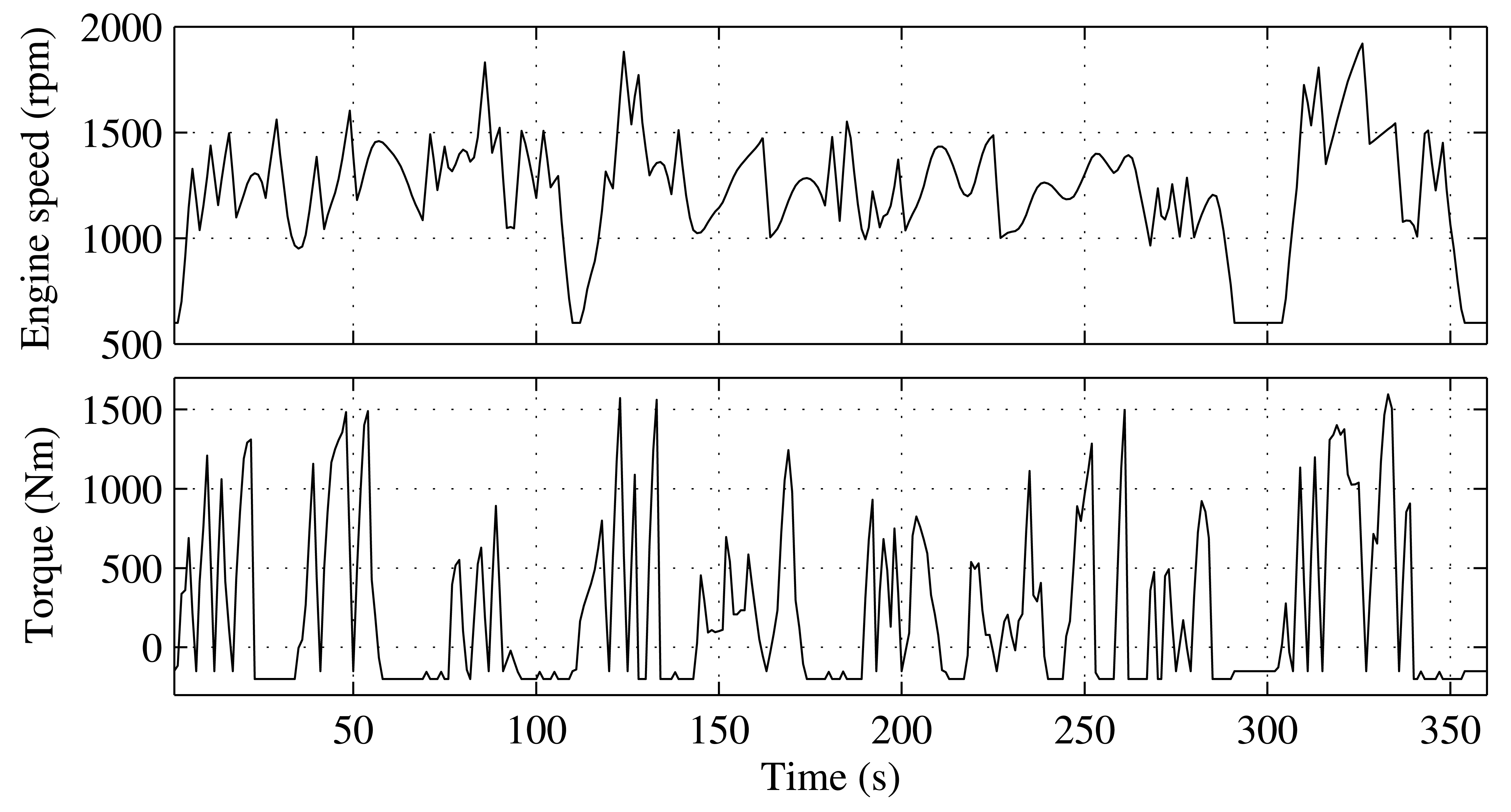
We consider an 8.71 turbocharged, heavy-duty diesel engine running a driving cycle lasting 1,800 s. It consists of five repetitions of a section of the urban part of the World Harmonized Transient Cycle (WHTC). Figure 1 shows one repetition of that section. The goal is the minimization of the CO₂ emissions, while keeping the NO_x emissions below the final value constraint, m_NOx,lim. The control input is the deviation of the crank angle for the start of injection (SOI) from its nominal value:

$$u=\delta {\phi }_{\text{SOI}}$$

(35)

In order to determine the optimal SOI and to simulate the engine on the driving cycle, an engine model is required that reproduces the influence of the SOI on the CO₂ and NO_x emissions. Because we are considering time scales in the order of entire driving cycles, the dynamics of the engine can be neglected, and the engine may be represented by a steady-state model with the inputs, engine speed ω_e, torque T and control input u,

$${\stackrel{*}{m}}_{{\text{CO}}_2}=f\left({\omega }_{\text{e}},T,u\right)$$

(36)

$${\stackrel{*}{m}}_{{\text{NO}}_x}=f\left({\omega }_{\text{e}},T,u\right)$$

(37)

The steady-state engine model, (36) and (37), is realized as a lookup table, which was derived from a validated dynamic engine model [34].

The driving cycle prescribes the engine speed, ω_e, and the torque, T. It is sampled with the step size Δt = 1 s, and it consists of N = 1,800 samples. The dynamics of the sole state variable x = m_NOx are discretized using the Euler forward integration scheme, such that a discrete-time optimal control problem is obtained.

$$\underset{u(\cdot )}{min}\left\{\text{∑}_{n=0}^{N-1}{\stackrel{*}{m}}_{{\text{CO}}_2}\left({\omega }_{\text{e}}(n),T(n),u(n)\right)\right\}$$

(38a)

such that

$$x(0)=0$$

(38b)

$$\begin{array}{cc}x(n+1)=x(n)+{\stackrel{*}{m}}_{{\text{NO}}_x}\left({\omega }_{\text{e}}(n),T(n),u(n)\right)\cdot \mathrm{\Delta }t,& n=0,\dots ,N-1\end{array}$$

(38c)

$$x(N)\le m_{{\text{NO}}_x,\text{lim}}$$

(38d)

This is an optimization problem of the structure of (9a)–(9d). Because it is time-discrete, it can be solved using dynamic programming (DP) [7]. That approach is guaranteed to find the optimal solution of the discretized problem. It can thus be used as a benchmark for the other approaches. As shown in Section 2.3, the dual formulation of the optimization can be solved alternatively,

$$\underset{u(\cdot )}{min}\left\{\text{∑}_{n=0}^{N-1}{\stackrel{*}{m}}_{{\text{CO}}_2}\left({\omega }_{\text{e}}(n),T(n),u(n)\right)+{\mathrm{\lambda }}_{{\text{NO}}_x}(n)\cdot {\stackrel{*}{m}}_{{\text{NO}}_x}\left({\omega }_{\text{e}}(n),T(n),u(n)\right)\right\}$$

(39)

This optimization problem has the same structure as (18a). Equations (18b)–(18c) are not necessary, because in this case, the engine model has no state variables. Given the optimal equivalence factor, the dual formulation (39) will produce the same solution as the DP. It can be solved online by minimizing the instantaneous equivalent emissions at every time step,

$$u(n)=\underset{u(n)}{\text{argmin}}\left\{{\stackrel{*}{m}}_{{\text{CO}}_2}\left({\omega }_{\text{e}}(n),T(n),u(n)\right)+{\mathrm{\lambda }}_{{\text{NO}}_x}(n)\cdot {\stackrel{*}{m}}_{{\text{NO}}_x}\left({\omega }_{\text{e}}(n),T(n),u(n)\right)\right\}$$

(40)

In the following, three different versions of EEMS are compared to the optimal solution obtained by DP. All three versions solve the minimization of the instantaneous equivalent emissions (40). They only differ in the way the equivalence factor is determined. The following three methods for determining the equivalence factor are considered:

• EEMS with constant equivalence factor (CEF): This method applies EEMS using the constant equivalence factor, which yields the correct final cumulated NO_x emissions. This equivalence factor can be obtained by an iterative simulation of the closed loop consisting of the engine model and the control law (40). Because the optimal control problems, (38a)–(38d) and (39), are equivalent, this method yields the same solution as the DP when the optimal equivalence factor is used. However, it is not applicable for causal control, because the optimal equivalence factor generally is not known.

• EEMS with operating-point dependent reference NO_x emissions (OPdep): This method applies EEMS using (32) to adapt the equivalence factor and (33) to calculate the reference NO_x emissions. The reference NO_x mass flow is calculated as a quadratic function of the operating point:

  $${\dot{m}}_{{\text{NO}}_x,\text{ref}}({\omega }_{\text{e}},T)=a_0+a_1\cdot {\omega }_{\text{e}}+a_2\cdot T+a_3\cdot {\omega }_{\text{e}}^2+a_4\cdot T^2+a_5\cdot {\omega }_{\text{e}}\cdot T$$

  (41)
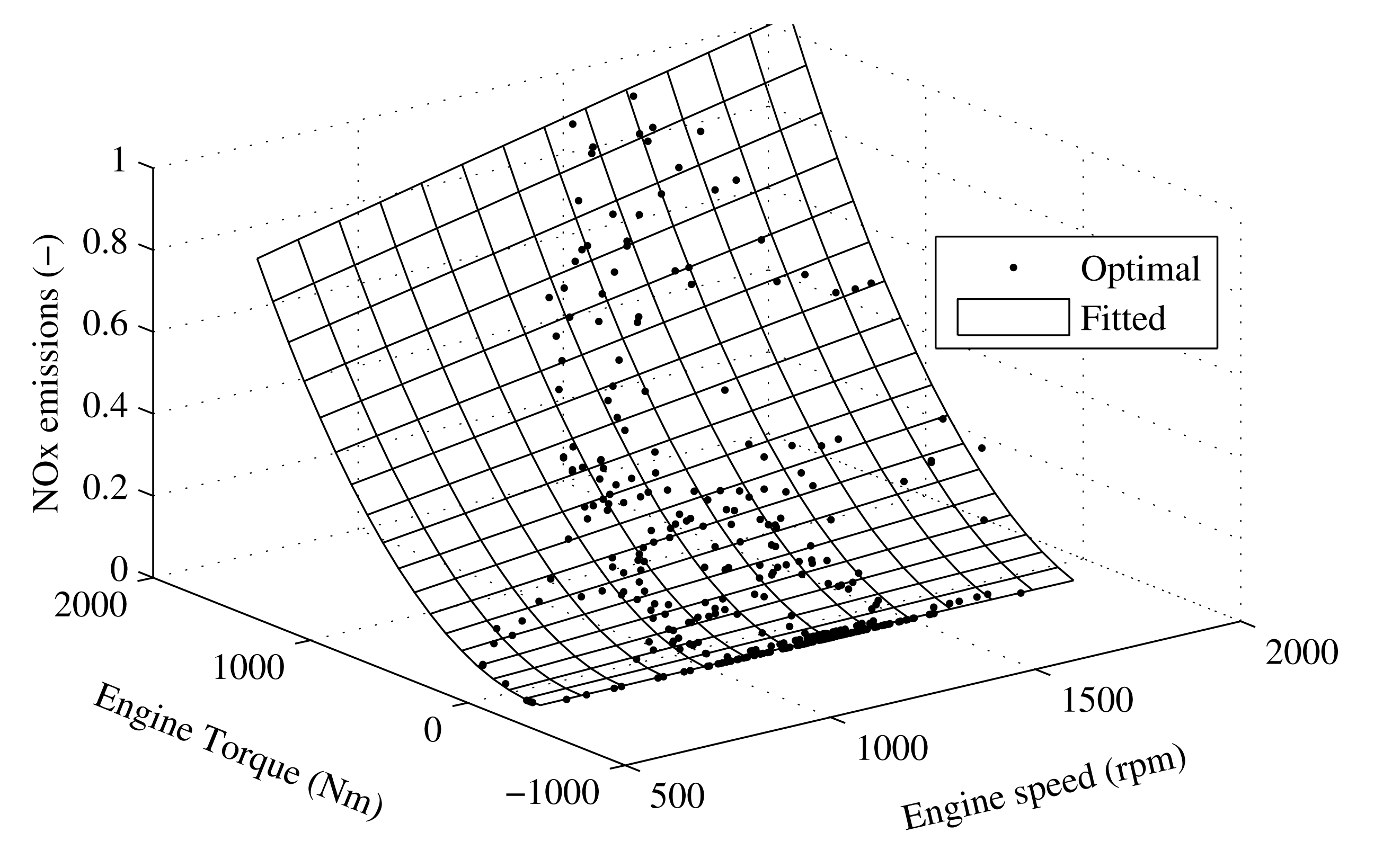
  The parameters, a₀ … a₅, are obtained by a least-squares fit of the NO_x emissions of the optimal solution obtained by DP. Figure 2 shows a comparison of the optimal NO_x emissions resulting from the DP and the fitted quadratic function. The quadratic model is a good approximation of the optimal values. However, this approach requires the availability of an optimal solution.

• EEMS with constant brake-specific reference emissions (BSconst): This method also applies EEMS using (32) to adapt the equivalence factor; however, it uses (34) to calculate the reference NO_x emissions. The reference value for the brake-specific NO_x emissions is equal to the average value, which was demanded for the DP solution:

  $${\overline{m}}_{{\text{NO}}_x,\text{ref}}=\frac{m_{{\text{NO}}_x,\text{lim}}}{W}=\frac{m_{{\text{NO}}_x,\text{lim}}}{{\text{∑}}_{n=0}^{N-1}{\omega }_{\text{e}}(n)\cdot T(n)\cdot \mathrm{\Delta }t}$$

  (42)

The two causal EEMS approaches, OPdep and BSconst, use the adaptation law (32) with identical tuning parameters, α˜ and T_int, for the adaptation of the equivalence factor. The tuning parameters were tuned manually.

4.2. Simulation Results

Figure 3 shows the simulation results of the non-causal DP and the three EEMS approaches when applied to the engine model, (36) and (37). The section of the WHTC is repeated five times. The optimal solution is a repetition of the optimal solution of the single section. The reason for this result is the fact that the only state variable represents the cumulated NO_x emissions, while the rest of the model does not depend on that state variable.

The first plot in Figure 3 shows the cumulated NO_x emissions of the different solutions. The NO_x mass has been normalized with the final value of the NO_x mass of the DP solution. The plot also shows the full range of attainable NO_x emissions, the upper limit corresponding to λ_NOx = 0 and the lower limit corresponding to λ_NOx = ∞. The cumulated NO_x emissions of all approaches are very similar, such that on the given scale, the respective lines cannot even be discerned. Therefore, the second plot shows the NO_x error:

$$\mathrm{\Delta }{\text{NO}}_x=m_{{\text{NO}}_x}-m_{{\text{NO}}_x,\text{dp}}$$

(43)

between the NO_x mass of the DP solution, m_NOx,dp, and the respective EEMS solution, m_NOx. Since the NO_x mass has been normalized, the NO_x error is normalized, as well.

As the results of the CEF approach show, the online solution of the dual problem (40) is equal to the offline solution of the constrained problem (38a)–(38d) when the optimal constant equivalence factor is used. This result confirms the theoretical result, which showed that the optimal equivalence factor of the cumulated pollutant emissions is always constant (15). Both causal EEMS approaches maintain the correct NO_x emission level by following the reference value for the NO_x emissions using feedback control. The cumulated NO_x emissions are kept within less than one percent of the final value.

The initial value, K₀, for the equivalence factor in (32) was chosen to be zero. After the second repetition of the section, the two controllers have converged to a limit cycle, and the behavior for all subsequent sections remains the same. The OPdep approach keeps both the equivalence factor and the emissions closer to the DP solution. This result is caused by the fact that the assumption of operating-point dependent reference emissions is more realistic than the constant brake-specific emissions.

The third plot of Figure 3 shows the CO₂ error:

$$\mathrm{\Delta }{\text{CO}}_2=m_{{\text{CO}}_2}-m_{{\text{CO}}_2,\text{dp}}$$

(44)

between the CO₂ mass of the DP solution, m_CO2,dp, and the respective EEMS solution, m_CO2. The CO₂ mass and the CO₂ error have been normalized with the final CO₂ mass of the DP solution. The plot clearly shows the trade-off between NO_x and CO₂ emissions. When the NO_x error increases, the CO₂ error decreases and vice versa. A large part of the CO₂ error is generated during the first two repetitions of the section before the EEMS controller has reached its limit cycle. In the beginning of the cycle, the equivalence factor is very low, and the engine is operated with a very high fuel efficiency, thus emitting large amounts of NO_x. Then, the NO_x emissions have to be reduced at a later point when the CO₂ penalty is larger than the amount saved in the beginning. However, once the controller has reached the limit cycle after two repetitions of the section, the CO₂ penalty of the causal EEMS controllers is small.

The performance of the various strategies can be compared by considering the cumulative emissions at the end of the cycle. In order to obtain a fair comparison and to eliminate the influence of the initial value of the equivalence factor, only the last three sections shown in Figure 3 are taken into account.

Table 1. Normalized difference Δ between the various strategies and the optimal DP strategy for the last three sections.

Strategy	ΔCO2 (%)	ΔNOx (%)
DP	0	0
EEMS OPdep	+0.032	−0.129
EEMS BSconst	+0.050	−0.104

shows the normalized results. Both causal EEMS approaches have only slightly higher CO₂ emissions than the DP solution. The NO_x emissions are even slightly lower for both strategies. The OPdep approach has both lower CO₂ and NO_x emissions than the BSconst approach, because the more realistic reference value leads to an equivalence factor that is closer to the optimal value. Generally, the performance of the causal EEMS approaches is very close to the non-causal, theoretical optimum.

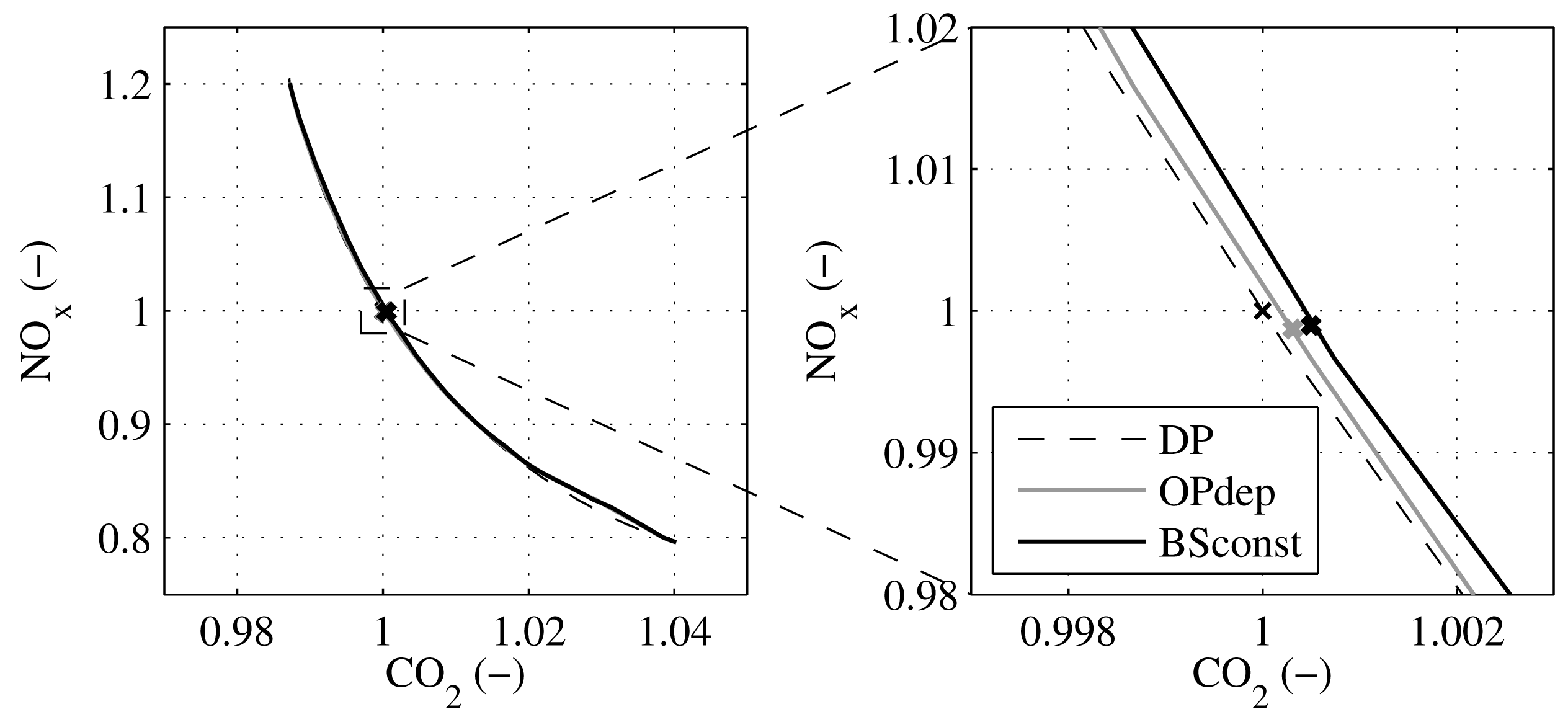
Finally, the performance of the various approaches for different reference NO_x emission levels is compared. Figure 4 shows the normalized trade-off between the cumulated CO₂ emissions and the cumulated NO_x emissions for the DP solution and the two causal EEMS approaches. The optimal trade-off can be obtained by varying the constant equivalence factor of the dual problem (39) or by varying the NO_x limit value of the original problem (38a)–(38d). The causal trade-off is obtained by setting the reference values for the causal EEMS controllers accordingly. Throughout the entire range, the Pareto front of the causal EEMS solutions is very close to the optimal Pareto front. These results show that the EEMS approach is well suited to an online optimization of the CO₂ and pollutant emissions of a diesel engine.

5. Conclusions

This paper presents a generic framework for the minimization of the CO₂ emissions of a diesel engine, while maintaining a certain pollutant emission level. It consists of an online adaptation of the equivalence factors in combination with a minimization of the equivalent emissions. First, it was shown that the constrained state variables associated with the pollutant emissions can be eliminated by minimizing the equivalent emissions instead. The optimal equivalence factors, which weigh pollutant emissions versus CO₂ emissions, are constant for a given cycle and emission limit. A method for the online adaptation of the equivalence factors was then derived using the HJB equation and a physically motivated approximation of the optimal cost-to-go function. Finally, a case study combined this adaptation method with an online minimization of the equivalent emissions. The performance of the proposed causal control strategies was very close to the theoretical non-causal optimum, which was determined using dynamic programming. This result confirmed that the EEMS framework is well suited to causal optimal control of the CO₂ and pollutant emissions of a diesel engine.

5.1. Outlook

The case study considered a static minimization of the equivalent emissions in combination with an adaptation of the equivalence factor. The results are very encouraging. In a next step, the EEMS framework could be applied to a more complex optimization problem. For example, additional control inputs, such as the injection pressure or additional injections, could be considered. In that case, the steady-state engine model (36)–(37) has to be extended in order to cover these inputs, as well. The optimization carried out in every time step (40) gains additional arguments. Its solution becomes computationally somewhat more expensive; however, it remains straightforward. Furthermore, the method used for the adaptation of the equivalence factor (32) remains the same.

Another topic worth pursuing is the realization of an EEMS with multiple pollutant emission limits. The implementation is straightforward; in addition to the weighted NO_x emissions, the dual formulation of the control problem (39) and the optimization carried out in every time step (40) contain terms for the other weighted pollutant mass flows. However, the solution of (40) does not become more complex. The additional equivalence factors are each adapted by an additional PI controller for the respective emission species (see (32)). It may prove advantageous to take into account the interaction among the various equivalence factors and the pollutant emissions by using a centralized multivariable controller instead of the individual PI controllers.

Furthermore, instead of the steady-state model (36)–(37), a dynamic engine model could be used for the optimization. The static optimization solved in every time step (40) is then replaced by a dynamic optimization of the structure of (18a)–(18c). The solution of such dynamic optimization problems for diesel engines is currently under research [8]. The computational cost is significantly higher than for the solution of a static optimization, such as (40). However, the method used for the adaptation of the equivalence factor (32) remains the same.

Finally, future research could aim at the combination of EEMS and ECMS for hybrid vehicles. As discussed in Section 3.3, the goal would be to achieve a fuel-optimal, charge-sustaining operation, while respecting the legislative limit for the pollutant emissions.

References

- International Energy Agency. CO2Emissions From Fuel Combustion—Highlights; IEA Publications: Paris, France, 2012. [Google Scholar]
- International Energy Agency. World Energy Outlook; IEA Publications: Paris, France, 2011. [Google Scholar]
- Intergovernmental Panel on Climate Change. Climate Change 2007: Synthesis Report. Contribution of Working Groups I, II and III to the Fourth Assessment Report of the Intergovernmental Panel on Climate Change; IPCC: Geneva, Switzerland, 2007. [Google Scholar]
- Rakopoulos, C.D.; Giakoumis, E.G. Diesel Engine Transient Operation—Principles of Operation and Simulation Analysis; Springer: London, UK, 2009. [Google Scholar]
- Heywood, J. Internal Combustion Engine Fundamentals; McGraw-Hill Series in Mechanical Engineering; McGraw-Hill: New York, NY, USA, 1988. [Google Scholar]
- Geering, H.P. Optimal Control with Engineering Applications; Springer: Berlin, Germany, 2007. [Google Scholar]
- Bertsekas, D.P. Dynamic Programming and Optimal Control, 3rd ed.; Athena Scientific: Belmont, MA, USA, 2005. [Google Scholar]
- Asprion, J.; Chinellato, O.; Guzzella, L. Optimal control of diesel engines: Numerical methods, applications, and experimental validation. Math. Probl. Eng. 2014. in press. [Google Scholar]
- Grahn, M. Model-Based Diesel Engine Management System Optimization—A Strategy for Transient Engine Operation. Ph.D. Thesis, Chalmers University of Technology, Gothenburg, Sweden, 2013. [Google Scholar]
- Benz, M.; Hehn, M.; Onder, C.H.; Guzzella, L. Model-based actuator trajectories optimization for a diesel engine using a direct method. J. Eng. Gas Turbines Power 2011, 133, 032806:1–032806:11. [Google Scholar]
- Kolmanovsky, I.; van Nieuwstadt, M.; Sun, J. Optimization of Complex Powertrain Systems for Fuel Economy and Emissions. Proceedings of the 1999 IEEE International Conference on Control Applications, Kohala Coast, HI, USA, 22–27 August 1999; Volume 1, pp. 833–839.
- Cloudt, R.; Willems, F. Integrated emission management strategy for cost-optimal Engine-Aftertreatment Operation. SAE Int. 2011. [Google Scholar] [CrossRef]
- Guzzella, L.; Onder, C. Introduction to Modeling and Control of Internal Combustion Engine Systems, 2nd ed.; Springer: Berlin, Germany, 2010. [Google Scholar]
- Hafner, M.; Schüler, M.; Nelles, O.; Isermann, R. Fast neural networks for diesel engine control design. Control Eng. Pract. 2000, 8, 1211–1221. [Google Scholar]
- Schär, C.M.; Onder, C.H.; Geering, H.P.; Elsener, M. Control-oriented model of an SCR catalytic converter system. SAE Int. 2004. [Google Scholar] [CrossRef]
- Devarakonda, M.; Parker, G.; Johnson, J.H.; Strots, V.; Santhanam, S. Adequacy of reduced order models for model-based control in a urea-SCR aftertreatment system. SAE Int. 2008. [Google Scholar] [CrossRef]
- Boyd, S.; Vandenberghe, L. Convex Optimization; Cambridge University Press: New York, NY, USA, 2004. [Google Scholar]
- Bemporad, A.; Morari, M.; Ricker, N.L. Model Predictive Control ToolboxUser's Guide; Mathworks: Natick, USA, 2013. [Google Scholar]
- Ambühl, D. Energy Management Strategies for Hybrid Electric Vehicles. Ph.D. Thesis, ETH Zürich, Zürich, Switzerland, 2009. [Google Scholar]
- Sciarretta, A.; Guzzella, L. Control of hybrid electric vehicles. IEEE Control Syst. Mag. 2007, 27, 60–70. [Google Scholar]
- Ambühl, D.; Guzzella, L. Predictive reference signal generator for hybrid electric vehicles. IEEE Trans. Veh. Technol. 2009, 58, 4730–4740. [Google Scholar]
- Johnson, V.H.; Wipke, K.B.; Rausen, D.J. HEV control strategy for real-time optimization of fuel economy and emissions. SAE Int. 2000. [Google Scholar] [CrossRef]
- Lin, C.C.; Peng, H.; Grizzle, J.W.; Kang, J.M. Power management strategy for a parallel hybrid electric truck. IEEE Trans. Control Syst. Technol. 2003, 11, 839–849. [Google Scholar]
- Lin, C.C.; Peng, H.; Grizzle, J.W. A Stochastic Control Strategy for Hybrid Electric Vehicles. Proceedings of the 2004 American Control Conference, Boston, MA, USA, 30 June–2 July 2004; Volume 5, pp. 4710–4715.
- Musardo, C.; Staccia, B.; Midlam-Mohler, S.; Guezennec, Y.; Rizzoni, G. Supervisory Control for NOx Reduction of an HEV with a Mixed-Mode HCCI/CIDI Engine. Proceedings of the 2005 American Control Conference, Portland, OR, USA, 8–10 June 2005; Volume 6, pp. 3877–3881.
- Ao, G.Q.; Qiang, J.X.; Zhong, H.; Mao, X.J.; Yang, L.; Zhuo, B. Fuel economy and NOx emission potential investigation and trade-off of a hybrid electric vehicle based on dynamic programming. Proc. Inst. Mech. Eng. Part D J. Automob. Eng. 2008, 222, 1851–1864. [Google Scholar]
- Sagha, H.; Farhangi, S.; Asaei, B. Modeling and Design of a NOxEmission Reduction Strategy for Lightweight Hybrid Electric Vehicles. Proceedings of the 35th Annual Conference of IEEE on Industrial Electronics, Porto, Portugal, 3–5 November 2009; pp. 334–339.
- Willems, F.; Spronkmans, S.; Kessels, J. Integrated Powertrain Control to Meet Low CO2 Emissions for a Hybrid Distribution Truck With SCR-Denox System. Proceedings of the ASME 2011 Dynamic Systems and Control Conference, Arlington, VA, USA, 31 October–2 November 2011; pp. 907–912.
- Johri, R.; Salvi, A.; Filipi, Z. Optimal Energy Management for a Hybrid Vehicle Using Neuro-Dynamic Programming to Consider Transient Engine Operation. Proceedings of the ASME 2011 Dynamic Systems and Control Conference, Arlington, VA, USA, 31 October–2 November 2011; pp. 279–286.
- Grondin, O.; Thibault, L.; Moulin, P.; Chasse, A.; Sciarretta, A. Energy Management Strategy for Diesel Hybrid Electric Vehicle. Proceedings of the 2011 IEEE Vehicle Power and Propulsion Conference, Chicago, IL, USA, 6–9 September 2011; pp. 1–8.
- Nüesch, T.; Wang, M.; Voser, C.; Guzzella, L. Optimal Energy Management and Sizing for Hybrid Electric Vehicles Considering Transient Emissions. Proceedings of the 2012 IFAC Workshop on Engine and Powertrain Control, Simulation and Modeling, Paris, France, 22–25 October 2012.
- Millo, F.; Ferraro, C.V.; Rolando, L. Analysis of different control strategies for the simultaneous reduction of CO2 and NOx emissions of a diesel hybrid passenger car. Int. J. Veh. Des. 2012, 58, 427–448. [Google Scholar]
- Serrao, L.; Sciarretta, A.; Grondin, O.; Chasse, A.; Creff, Y.; Di Domenico, D.; Pognant-Gros, P.; Querel, C.; Thibault, L. Open issues in supervisory control of hybrid electric vehicles: A unified approach using optimal control methods. Oil Gas Sci. Technol. Rev. IFP Energies Nouv. 2013, 68, 23–33. [Google Scholar]
- Asprion, J.; Chinellato, O.; Guzzella, L. Optimisation-oriented modelling of the NOx emissions of a diesel engine. Energy Convers. Manag. 2013, 75, 61–73. [Google Scholar]