DVP: A Novel High-Availability Seamless Redundancy (HSR) Protocol Traffic-Reduction Algorithm for a Substation Automation System Network

Abstract
: The high-availability seamless redundancy (HSR) protocol, a potential candidate for substation automation system (SAS) networks, provides duplicated frame copies of each sent frame, with zero fault-recovery time. This means that even in the case of node or link failure, the destination node will receive at least one copy of the sent frame. Consequently, there is no network operation down time. However, the forwarding process of the QuadBox node in HSR is not smart and relies solely on duplication and random forwarding of all received frames. Thus, if a unicast frame is sent in any closed-loop network, the frame copies will be spread through most of all the links in both directions until they reach the destination node, which inevitably results in significant, unnecessary network traffic. In this paper, we present an algorithm called the dual virtual paths (DVP) algorithm to solve such an HSR excessive traffic issue. The idea behind our DVP algorithm is to establish automatic DVP between each HSR node and all the other nodes in the network, except for the QuadBox node. These virtual paths will be used for DVP unicast traffic transmission, rather than using the standard HSR transmission process. Therefore, the DVP algorithm results in less traffic, because there is no duplication or random forwarding, contrary to standard HSR. For the sample networks selected in this paper, the DVP algorithm shows more than a 70% reduction in network traffic and about an 80% reduction in the discarded traffic compared to the standard HSR protocol.1. Introduction
Seamless communication with fault tolerance is one of the key requirements for an Ethernet-based mission-critical and real-time power system, such as substation automation system (SAS) networks. A fault-tolerant Ethernet (FTE) eliminates the single point of failure and, therefore, improves overall system availability [1]. Since standard Ethernet does not provide a fault-tolerance capability, various FTE protocols for power applications have been developed [2]. Among these, only two protocols, the parallel redundancy protocol (PRP) and the high-availability seamless redundancy (HSR) protocol, standardized as IEC62439-3, are suitable for seamless communication [2–4]. Both HSR and PRP are based upon the same principle of active redundancy by duplicating the information frames, which, therefore, results in a zero-delay re-configuration in case of a switch or link failure. However, in this paper, only the HSR protocol is covered, because it is generally accepted as the developed version of the PRP. As an example, in [5], Tan and Luan conclude that HSR-based implementation will dominate in future power-related applications, due to its excellent performance and affordable cost. The HSR protocol is a redundancy protocol for Ethernet-based networks, and it provides duplicated frame copies for each frame sent. In other words, the HSR protocol provides two frame copies for the destination node, one from each side, enabling zero-fault recovery time in case one of the frame copies is lost. This means that even in the case of a node or a link failure, there is no stoppage of network operations. If both sent copies reach the destination node, then it will take the fastest copy and discard the other copy. This feature of the HSR protocol makes it very useful for time-critical and mission-critical systems, such as SAS. Moreover, the HSR protocol is a Layer 2 protocol and is independent of the upper layer protocols, thus returning high flexibility in a wide range of different applications on HSR networks. The HSR-based network has four types of nodes [3]:
A doubly-attached node for HSR (DANH), which has two HSR ports sharing the same medium access control (MAC) and Internet protocol (IP) set addresses. This allows the address management protocols, such as the address resolution protocol (ARP), to operate as usual without modification, which simplifies network engineering. Each DANH node will duplicate a non-HSR frame that is generated at the upper layer into two frame copies. It will then append an HSR tag to each copy and send two copies out through DANH ports, one in a clockwise direction and the other in a counter-clockwise direction;
A single-attached node (SAN), which is a non-HSR device, such as a commercial printer, server or laptop, cannot be directly inserted into the HSR networks, since they lack the forwarding capability of an HSR node and do not support the HSR tag. They must be attached through a redundancy box (RedBox) node type;
A RedBox node has three ports: two of them are HSR ports, and the third one is an Ethernet port that any SAN device, such as a PC, can be plugged into to be engaged with the HSR network. The RedBox node forwards the frames over the HSR network like any other HSR node and acts as proxies for all SANs that access them. To this effect, they must keep track of all traffic on behalf of the SANs. The RedBox can also act as a switch for the SANs. Therefore, it is somewhat more complex than HSR nodes;
A quadruple port device (QuadBox node) has four HSR ports, and each pair of them shares the same MAC and IP addresses. This type of node is used to connect two rings or networks with each other. The QuadBox node removes duplication and does additional tasks, such as multicast and virtual local area network (VLAN) filtering.
Other HSR principles are examined and discussed in [3–8]. However, the HSR protocol is not free from drawbacks. A major one affecting its performance is the unnecessary redundant traffic caused by the duplicated frames that are generated and traveling inside the network. This downside divides the available network bandwidth for network traffic roughly in half, degrades network performance and may cause network congestion or even stoppage. Formerly, in 2012, we proposed two approaches to improve the HSR traffic performance by reducing the unnecessary traffic in HSR networks [9]. The first approach is called quick removing (QR) for ring-type (single ring or connected rings) networks. This approach, simple and therefore easy to implement, shows up to a 50% multi/broadcast traffic reduction compared to the standard HSR protocol. The second approach is the virtual ring (VRing), which involves dividing any closed-loop-type HSR network into several VRings. This VRing approach shows a network-traffic reduction in the range of about 50%–70% in a failure-free case and about 40%–90% in a failure case, as compared to the standard HSR protocol. In addition, we showed that QR and VRing could be applied together to get a greater reduction. Note that, however, the VRing requires a static configuration, which needs the network administrator's intervention. Later, we also proposed a different approach, called removing the unnecessary redundant traffic (RURT), for any HSR closed-loop network type at an early stage [10]. For the sample network, the RURT approach shows up to a 50% reduction in network traffic under both failure-free and failure cases compared to the standard HSR protocol. The RURT works in any closed-loop network, so it is an enhanced version of the QR approach. Our algorithm details and engineering issues can be found in [6]. Abdulsalam and Rhee proposed a practical unicast traffic-reduction method, called the port locking (PL) algorithm, for the connected-rings configuration network [11]. Hong and Joe introduced a packet transmission scheme with different periods based on a single ring topology for reducing the HSR network-traffic load [12].
In this paper, we present a novel algorithm, called the dual virtual paths (DVP) algorithm, to improve the HSR network performance by reducing the unnecessary redundant unicast traffic type in any HSR closed-loop network. These network types always face the problem of duplicating every sent unicast frame at each QuadBox node type available in the network, then forwarding these frames randomly toward the destination, which leads to many frame copies circulating in the network. Eventually, the destination node receives only two of these frames, taking the fastest one and discarding the second, whereas the other circulating frame copies are deleted and removed from the network as soon as they pass twice through the same node and in the same direction. Here, dual paths are chosen in order to accommodate two duplicated HSR frames for each sending frame. The DVP algorithm establishes two virtual paths between each DANH or RedBox node type and the other DANH or RedBox nodes if they are available in the same network. Eventually, a virtual full-mesh network is established among all the DANH and RedBox nodes, except for the QuadBox nodes, because this type is only used for interconnecting purposes and does not have any attached end users. The DVP algorithm significantly reduces the total network traffic by more than 70% and improves the network performance, as shown in Sections 3 and 4.
The rest of the paper is organized as follows. In Section 2, we briefly introduce the DVP algorithm and its concept. In Section 3, the analytical traffic performance for the standard HSR protocol and the DVP algorithm is calculated and compared for different cases. In Section 4, the simulated traffic performance is carried out and compared for different cases. Finally, in Section 5, we provide our conclusions and suggestions for future work.
2. The DVP Algorithm
2.1. DVP Concepts
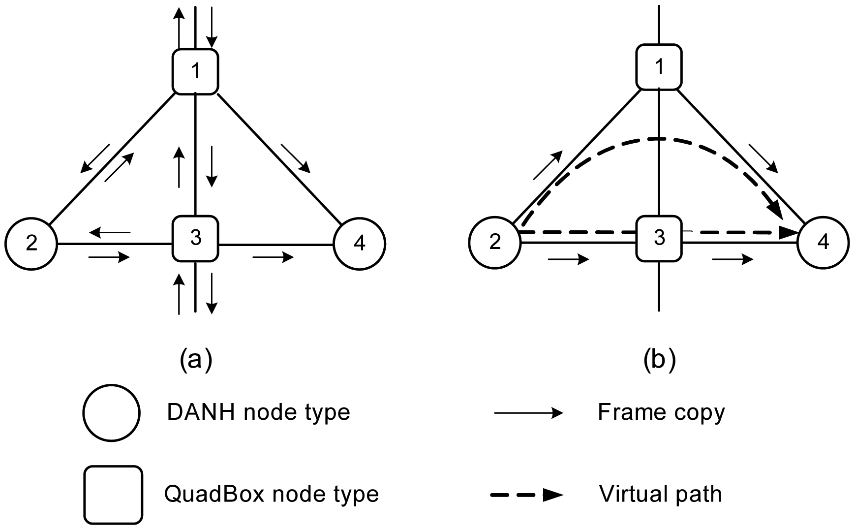
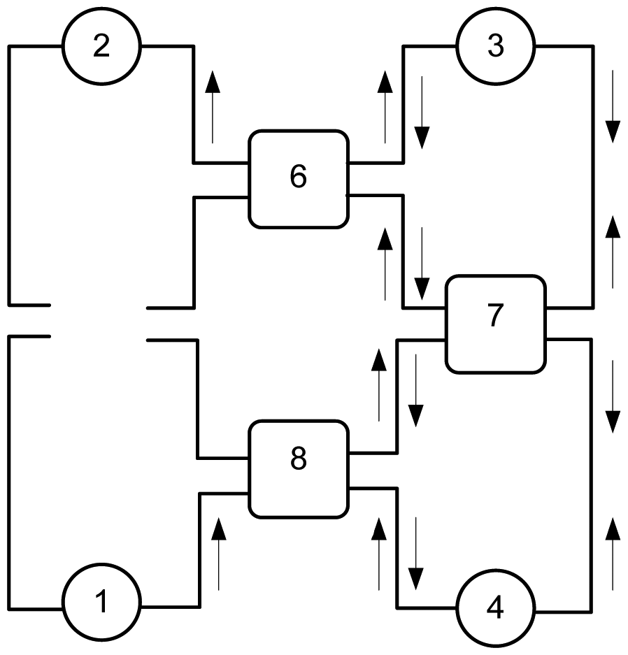
The primary goal of the DVP algorithm is to make the DANH and RedBox nodes in an HSR network capable of communicating with each other using a connection pair (point-to-point connection) instead of using the standard HSR transmission process of duplication and random forwarding at each QuadBox node until the sent copies reach the required destination. The DVP establishes two virtual paths between each pair of DANH or RedBox nodes. Note that a DANH node can establish paths with a RedBox node, or vice versa. However, these paths will be established automatically through a certain procedure, which will be described in the DVP setup process. Such a process simply makes all of the QuadBox nodes “smart” after a learning task. The nodes then understand how to forward the received fastest frame of each connection pair to the proper destination through only one of their ports, instead of duplicating and forwarding the frame randomly through all the ports, except for the port from which the frame has been received. An example in Figure 1 describes the key idea of the DVP algorithm compared to the standard HSR protocol.
Figure 1a shows the HSR frame distribution under the condition of sending a single frame from Node 2 to Node 4. However, due to the operational concepts of the QuadBox (duplication and forwarding) Nodes 1 and 3, each of the network links, except for the destination node's links, has two frame copies, one in each direction. The matter is different in the network shown in Figure 1b, which makes use of the DVP algorithm. The difference arises because Node 2 has established two virtual paths with Node 4 for sending and receiving the unicast traffic type. These virtual paths are: Node 2-Node 3-Node 4 and Node 2-Node 1-Node 4. Each of theses paths transfers only one frame copy from Node 2 to Node 4 without any duplication or random forwarding, as in the standard HSR protocol, because the QuadBox Nodes 1 and 3 have learned through a learning process how to forward the unicast frame type from Node 2 to Node 4. The frame distribution in Figure 1a,b is drawn in such a way as to show all the frame copies that are traveling in the network during the time period, from sending the frame to receiving or deleting all the frame copies.
2.2. DVP Frame Structure
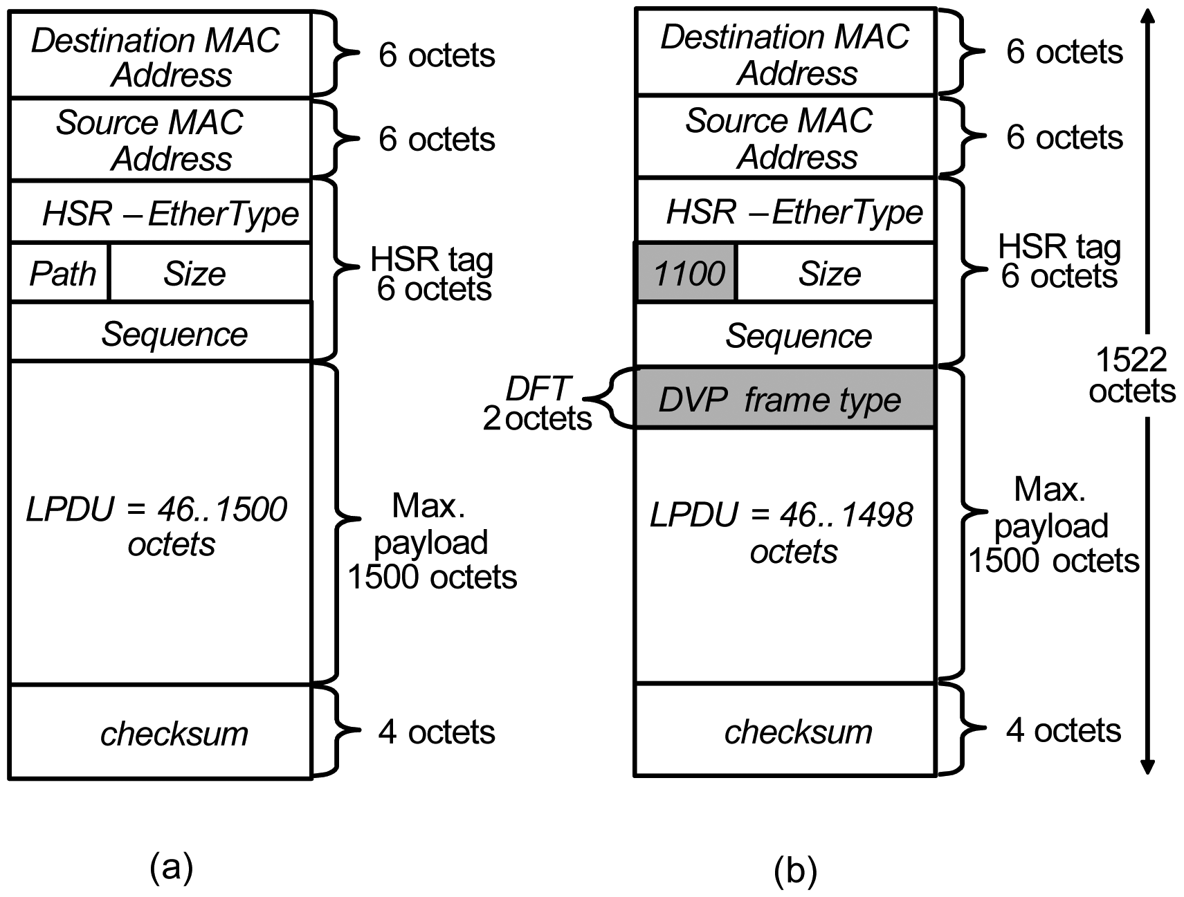
The DVP algorithm uses several types of special frames; each has a certain purpose and a mission that needs to be accomplished. To allow the HSR nodes to differentiate between these frames when the DVP is running, we inserted a new field inside the payload of the standard HSR frame within a unique code for each of these special frames. This field is called the DVP frame type (DFT), as shown in Figure 2, and it has the size of two octets. The location of the DFT field inside the payload is intended to preserve the entire DVP special frame at the standard HSR size.
However, to differentiate between the standard HSR frames and the DVP frames (each of which has a unique DFT code), it is necessary to set a certain flag or a code inside the header of each DVP frame. For this purpose, we used one of the reserved codes of the path identifier field that is located inside the standard HSR frame header. Code 1100 refers to a special DVP frame. In the absence of this code, the node would consider the received frame as a standard HSR frame.
2.3. Three DVP Phases
The DVP algorithm is composed of three phases, as described below, to make it easy to understand, track, implement and upgrade in the future. Note that in the network start-up, all the nodes will use the standard HSR protocol until they complete the DVP setup process, after which, they use the DVP.
2.3.1. Announcement Phase
This is the first phase and can be summarized as follows:
Each terminal node will announce itself by broadcasting a special DVP frame called the announcement (Ann.) frame;
The Ann. frame copies will spread through the network from node to node, until each copy goes back to the source node or passes twice through the same node and in the same direction before being deleted and removed from the network;
All the network nodes, including the QuadBox node type, will read each passing Ann. frame copy;
Then, a table, called the neighbors (Ne) table, will be built. The Ne table contains the source MAC address and the sequence number of each read Ann. frame.
2.3.2. Paths Establishment Phase
The second phase can be summarized as follows:
All the terminal nodes will establish dual virtual paths with each other and use them for point-to-point communication instead of spreading their data frames through the network, as in the standard HSR protocol;
This task will be done by teaching the QuadBox nodes how to forward or guide the received frames to their sources or destination nodes without duplicating and forwarding them randomly. This mission is accomplished by sending a special DVP frame from each terminal node to each node listed in its Ne table. This frame is called the path selection (PaS) frame;
Then, each node will save the information of each virtual path for each connection pair in a table called the final paths (FP) table. This table will show the input and the output port for each path.
As an important feature of the DVP algorithm, the dual virtual paths of each connection pair shall be separated to ensure that if one of the paths is down, the other will not be impacted. Therefore, the terminal nodes of each connection pair shall ensure that this criterion is met during the FP table-building task; else, it will re-establish the virtual paths through a particular procedure to avoid the availability of common nodes.
2.3.3. Final Phase
Each frame copy, after duplication, will then be sent to a virtual path that has been established earlier with that destination terminal node. Each QuadBox node will be able to forward the received data frames to their destination or to source terminal nodes by using its FP table instead of the standard HSR transmission process.
Generally, if a QuadBox node, for one of any number of reasons, cannot find the proper output port for a particular received frame in its FP table, then it will duplicate and forward the frame copies randomly to the next nodes, as in the standard HSR transmission process. Thus, in this way, the DVP algorithm ensures it will not discard or delete any received frame, and the destination node will receive at least one copy from that frame. However, if a QuadBox node receives a broadcast or a multicast data frame, it will use the standard HSR transmission process of duplication and random forwarding.
2.4. Monitoring and Repairing Paths Failures
The DVP algorithm supports continuous monitoring of the health status of the dual virtual paths of all the connection pairs to ensure they are functioning properly and failure-free. This will involve sending a special DVP frame, called the path health checking (PHC), frame from each terminal node to the corresponding node in the same connection pair. The sending process will occur periodically during the final phase. However, the health status of the other network nodes that are not located on any virtual path will not be visible in the PHC frame. Therefore, the DVP algorithm will use the supervisory frame for this purpose, because this frame type will be spread through the network, since it is a multicast frame type, and then, the network administrator server (or the control station) will receive at least one copy from each node's supervisory frame every two seconds, according to the standard HSR protocol. In this way, the network administrator will receive the supervisory frames independently from the status of the virtual paths, and will know the status of each network node.
2.5. Path Re-Establishment
If a terminal node discovers that a link or node is dead, because it did not reply to its PHC frame, then the node will run the path re-establishment procedure with the corresponding node to re-establish the dual virtual paths with it. This procedure will be accomplished by sending a special DVP frame, called the re-path selection (RePaS), frame from a terminal node of a connection pair to the corresponding node in the same pair, asking it to re-send the PaS frame, or in other words, to re-establish new virtual paths with it. However, with the DVP algorithm, any virtual path-failure due to a link-failure case will be repaired within less than one millisecond, according to our simulation result of the sample network shown in Figure 3.
3. Traffic Performance Analyses
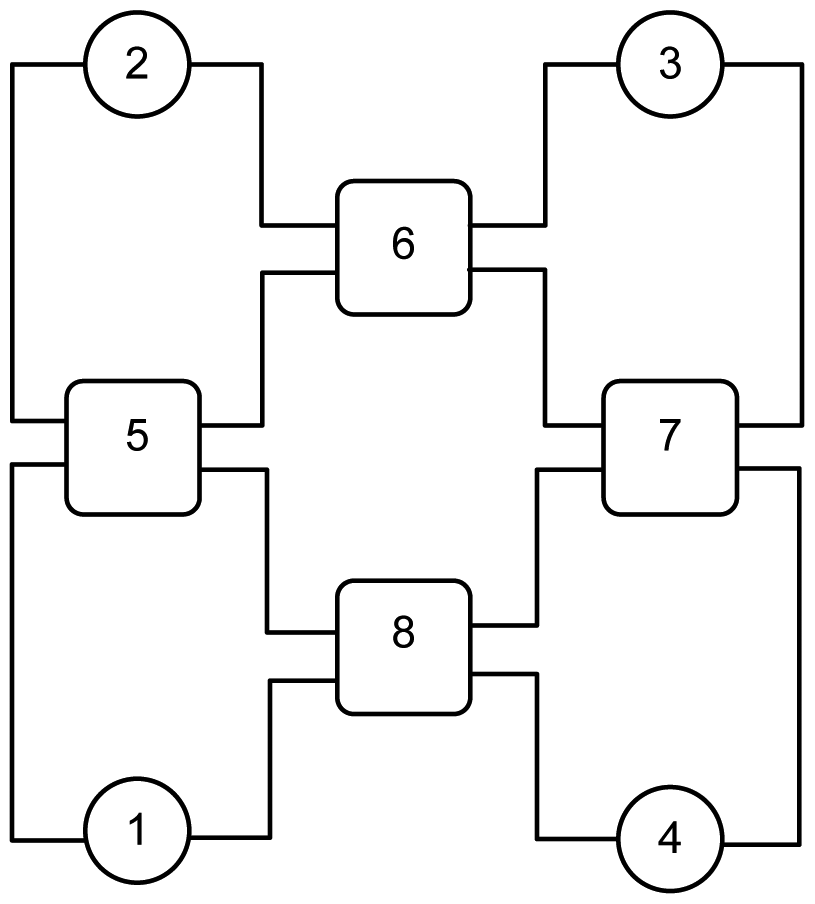
To evaluate the performance of the DVP algorithm compared to the standard HSR protocol, the network-traffic parameter is chosen as a performance metric, since it will show a clear difference between the two algorithms from the point of view of traffic reduction. The network-traffic parameter represents the total number of frame copies that travel in a network during the duration time that starts from sending the frames, until receiving or deleting all of them. The sample network shown in Figure 3 has been used throughout this paper for both analytical derivations and experimental simulations. This network has enough complexity to show the performance comparison between the two algorithms. Furthermore, the configuration of the sample network covers most industrial automation network configurations, including the SAS. The methodology presented in this paper can be easily extended to other network configurations.
3.1. Network Traffic Analyses
As mentioned in Section 1, the DVP algorithm only works with the unicast traffic type; therefore, unicast traffic will be covered in this paper. However, the DVP algorithm's behavior with multi-broadcasting traffic will be similar to the standard HSR protocol, which only depends on the duplication and random forwarding of the received frames at each QuadBox node until they reach the destination, or until they pass twice through the same node and direction to be deleted and removed from the network [9].
In this section, analytical expressions for the network traffic will be derived under various cases with three scenarios for the sample network shown in Figure 3. These three scenarios are as follows:
Scenario I: unicast single frame transmission to an adjacent node;
Scenario II: unicast single frame transmission to a separated node;
Scenario III: generalization and unicast multiple frame transmission to corresponding nodes according to Table 1.
3.1.1. Network Traffic under the Standard HSR Protocol
The following cases will be considered when deriving the analytical expressions for the network traffic under both the standard HSR protocol and DVP algorithm:
- (a)
Failure-Free Case Under the Standard HSR Protocol.
This case means that all the links and the nodes will be working properly and are failure-free. The following communication scenarios will be used in all cases:
- Scenario I:
Assume that Node 1 sends a unicast frame to Node 2; then, the traffic distribution will be as shown in Figure 4. The total network traffic due to the first scenario will be equal to
where tfu12 is the total unicast frame copies that are traveling in the network under a standard HSR protocol due to communication between Nodes 1 and 2; f12 is the total unicast frames sent by Node 1 to Node 2, which is equal to one frame in this case; and l is the number of failure-free network links equal to twelve links.Therefore, tfu12 = 1 × ((2 × 12) − 3) = 21 frame copies.
- Scenario II:
Assume that Node 3 sends a unicast frame to Node 1 that is not directly adjacent to Node 3. Then, the total unicast traffic due to the second scenario will be equal to:
- Scenario III:
Equation (3) will be used to calculate the total unicast traffic that might be traveling in the network shown in Figure 3, due to it sending any unicast frames from any terminal nodes:
where tfu is the total number of unicast frame copies that are traveling in the network under a standard HSR protocol; fij is the total number of unicast frames sent from Node i to Node j and adj is called the adjacent factor which is equal to zero if Node i and Node j are directly connected to a common adjacent node; otherwise, it is equal to one, and n is the number of the terminal nodes.If we assume that each of the terminal nodes in the sample network has sent one unicast frame to the destinations described in Table 1, then the total network frame copies in this case can be calculated by using Equation (3) as follows:
- (b)
Link-Failure Case Under the Standard HSR Protocol.
Assume the link between Nodes 1 and 5 has failed during network operation and that the failure state stays for a long time as a worse situation under this case. The same previous scenarios will also be used in this case to compare the results with the failure-free case.
- Scenario I:
For the first scenario of Nodes 1 and 2, Equation (1) is still valid to calculate the network traffic for this case, but with a slight modification:
where tfu12l f is the total number of unicast frame copies that are traveling in the network due to communication between Nodes 1 and 2 under a standard HSR link-failure case and ll f is the number of failure-free links under the link-failure case.Since f12=1 and ll f = 11, therefore, tfu12l f becomes 19 frame copies.
- Scenario II:
For this scenario, the traffic will be:
- Scenario III:
For a general case, the following equation can be made:
where tful f is the total number of unicast frame copies that are traveling in the network under a standard HSR protocol–link-failure and adjl f is the adjacent factor under the link-failure case. adjl f is zero if Node i and Node j are directly connected to a common adjacent node; otherwise, it is equal to two.For the scenario in Table 1, the total network traffic under this case, tful f, becomes 76 frame copies.
- (c)
Node-Failure Case Under the Standard HSR Protocol.
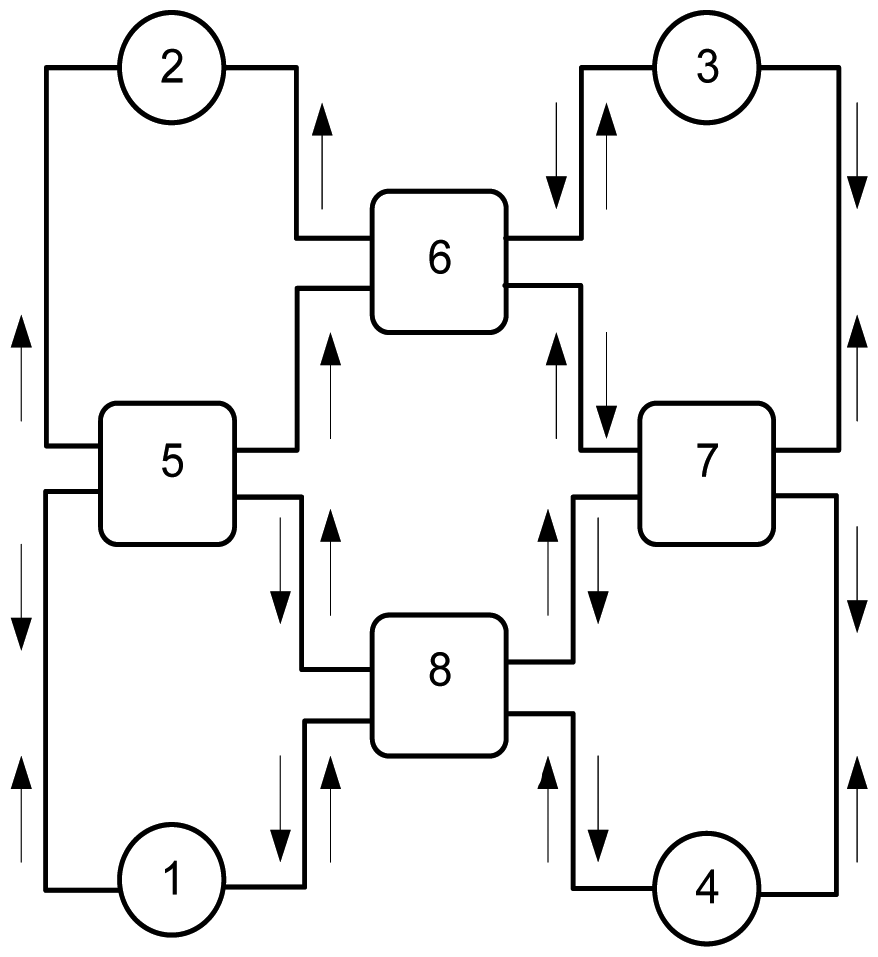
When one of the QuadBox nodes has failed, the effects on the network operation are more severe than any terminal node case, since four links are connected with each QuadBox, whereas only two links are connected with each terminal node. Let us assume that Node 5 has failed during network operation, and the failure state stays for a long time, as a worse situation under this case. The failure of Node 5 will cause all the links that are connected to it to fail, and this failure will cause the deletion of one of the two circulating frames (one in each direction) for some links, as shown in Figure 5.
- Scenario I:
For this scenario, Equation (4) will be modified as follows:
where tfu12n f is the total number of unicast frame copies that are traveling in the network due to the communication between Nodes 1 and 2 under a standard HSR node-failure case and ln f is the number of failure-free links under the node-failure case.Since ln f = 8, then tfu12n f = 14 frame copies.
- Scenario II:
In the same way, the traffic under the second scenario will be:
- Scenario III:
The total traffic can be expressed as:
where tfun f is the total number of unicast frame copies that are traveling in the network under a standard HSR protocol–node-failure and adjn f is the adjacent factor under the node-failure case. adjn f is equal to zero if:Node i is one or two and Node j is three or four;
or Node i is three or four and Node j is four or three.
Otherwise, it is equal to three if:
Node i is three or four and Node j is one or two;
or Node i is one or two and Node j is two or one.
For the scenario in Table 1, the total number of frame copies, tfun f, becomes 50 frame copies.
3.1.2. Network Traffic under the DVP Algorithm
The same cases that have been used in the standard HSR will be applied in this section.
- (a)
Failure-Free Case Under the DVP Algorithm.
Here, it is assumed that all the links in the network have the same lengths.
- Scenario I:
For the first scenario of Node 1 sending a unicast frame to Node 2, the first fastest path for the PaS frame sent from Node 1 to Node 2 (PaS1) will be Node 1-Node 5-Node 2 and the second path will be Node 1-Node 8-Node 7-Node 6. Regarding the fastest path for the PaS frame sent from Node 2 to Node 1 (PaS2), the path will be Node 2-Node 5-Node 1, which is the same first path for PaS1, and the second path will be Node 2-Node 6-Node 7-Node 8-Node 1, which is also the same second path for the PaS1 frame.
The network traffic of the DVP algorithm can be expressed as follows:
where tfu12−d is the total unicast frame copies between Nodes 1 and 2 under the DVP algorithm, lp1,12 is the number of links in the first path between Nodes 1 and 2 and lp2,12 is the number of links in the second path between Nodes 1 and 2.Since lp1,12 = 2 and lp2,12 = 4, then tfu12−d = 6 frame copies.
- Scenario II:
For the scenario of Node 3 sending a unicast frame to Node 1, the traffic will be:
Note that the dual paths between this connection pair can be obtained from the simulation tool or from the network diagram, because all the link segments have the same length. Thus, tfu31−d = 6 frame copies.
- Scenario III:
The generalized traffic can be expressed as:
where tfu−d is the total number of unicast frame copies under the DVP algorithm, lp1,ij is the number of links in the first path between Nodes i and j and lp2,ij is the number of links in the second path. For the scenario in Table 1, tfu−d will be calculated from Equation (12) as follows,Since f13 = f24 = f32 = f41 = 1, and all of the connection pairs have two links for the first path and four links for the second path, then tfu−d becomes 24 frame copies.
- (b)
Link-Failure Case Under the DVP Algorithm.
- Scenario I and II:
The network traffic can be calculated from the following equations:
where tfu12−dl f is the total unicast frame copies between Nodes 1 and 2 under the DVP algorithm link-failure case; lp1l f,12 is the number of links in the first path between Nodes 1 and 2 under the link-failure case and lp2l f,12 is the number of links in the second path between Nodes 1 and 2 under the link-failure case.We find that lp1l f,12 = 0, because the link between Nodes 1 and 5 is down, and the sent frame could not travel along this path by even one link segment. In addition, lp2l f,12 = 4. Therefore, we get tfu12−dl f = 4 frame copies.
In the same way, we get tfu31−dl f = 1 × (2 + 3) = 5 frame copies. Note that lp1l f,31 = 2, because the sent frame copy from Node 3 could not travel through the first path (Node 3-Node 6-Node 5-Node 1) until it reached Node 5 and was then discarded, which means it could travel to two links before it was discarded.
- Scenario III:
The general traffic expression will be:
where tfu−dl f is the total unicast frame copies under the DVP algorithm link-failure case. For the scenario in Table 1, the tfu−dl f will be equal to 20 frame copies.
- (c)
Node-Failure Case Under the DVP Algorithm.
- Scenario I and II:
Equations (13) and (14) can be rewritten as follows:
where tfu12−dn f is the total number of unicast frame copies between Nodes 1 and 2 under the DVP algorithm node-failure case; lp1n f,12 is the number of links in the first path between Nodes 1 and 2 under the node-failure case and lp2n f,12 is the number of links in the second path under the node-failure case. Then tfu12−dn f = 1 × (0 + 4) = 4 frame copies andtfu31−dn f = 1 × (1 + 3) = 4 frame copies.
- Scenario III:
The general expression for this scenario is:
where tfu−dnf is the total number of unicast frame copies under the DVP algorithm node-failure case. For the scenario in Table 1, the total traffic will be equal to 14 frame copies.
3.2. Traffic Comparison
This section summarizes the DVP analytical results compared to the standard HSR, which are shown in Tables 23 and 4. From the discussed cases with three scenarios, it can be concluded that the DVP algorithm always outperforms the standard HSR protocol.
4. Traffic Performance Simulations
To validate the analytical results derived in Section 3, multiple simulations have been carried out for the sample network shown in Figure 3 by using a network simulation tool, OMNeT++v4.2.2. [13]. In order to accomplish the simulations, we have built each of the DANH and QuadBox node models into the simulation environments using C++ coding to perform their functions under both the standard HSR protocol and our DVP algorithm.
4.1. Simulation Experiments
Two types of experimental simulations have been undertaken to validate our DVP algorithm.
4.1.1. First Experiment
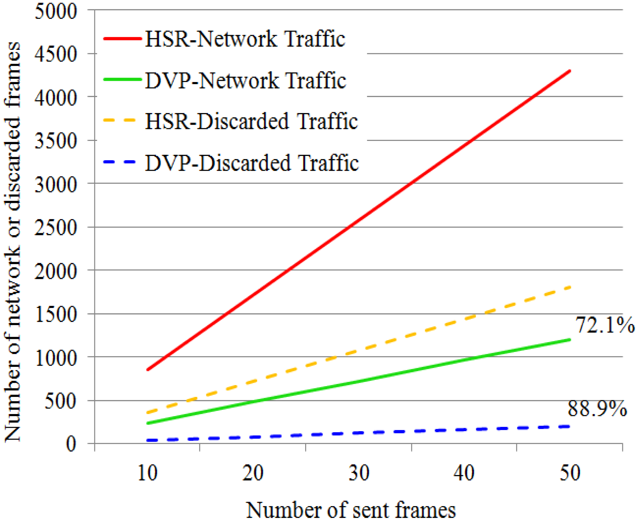
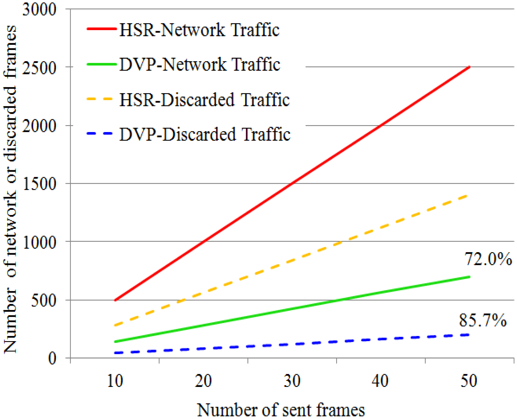
The network traffic for all of the cases with the three scenarios that have been analyzed in Section 3 have been simulated with our established simulation environment, and the results exactly matched the theoretical derivations. Therefore, instead, in this section, the simulations of the discarded traffic, which represent the discarded and deleted frames from all the network nodes, have been made, because discarded traffic also directly affects the network nodes' performance and makes them constantly busy with the process of discarding and deleting the unnecessary frames. It seems that the analytical expression for such discarded traffic cannot be easily obtained mathematically. The sample network of Figure 3 is used in this experiment with a scenario similar to the scenario in Table 1, but with different numbers of sent frames. Five tests have been conducted for this experiment under each failure-free and failure case. During the first test, 10 frames are sent from each sending node, then increased by 10 for each new test, until reaching 50 frames. The results of this experiment are illustrated in Figures 67 and 8, which represent the network and discarded traffic under both the standard HSR protocol and the DVP algorithm.
4.1.2. Second Experiment
In this experiment, we demonstrate that the DVP algorithm shows much better traffic performance when the network size increases. This is because the DVP algorithm guides the sent frames to their destination nodes through the DVP without duplicating and random forwarding, as in the standard HSR protocol. The sample network shown in Figure 9 is used to prove the above-mentioned goal. However, this network consists of 4 bay-level rings connected to a station-level ring. In addition, each bay ring consists of 20 DANH nodes.
The scenario of Node 1 sending a single frame to Node 41 is adopted in this simulation. Several tests are accomplished; each time, the number of the bay rings that are connected to the station ring is increased until it reaches 250. Figure 10 shows how the percentage for the network-traffic reduction varies with the network size. For example, when the network has 8 bay rings, the reduction was about 85%, while the percentage jumps to about 97% when the number of the connected bays is increased to 250 rings.
4.2. Discussion
It is shown from all the simulation results that the traffic performance of the DVP algorithm is much better than the standard HSR protocol. Throughout the simulations, we assumed that a failure would occur and stay for a long time, which demands a unified condition for both the DVP and standard HSR protocol for comparison purposes. In practical terms, the DVP will re-establish other paths automatically without any intervention by the network administrator, whereas the standard HSR protocol might suffer from the heavy, redundant traffic, since it does not have a sufficient number of paths to distribute it. As shown in our simulation experiments, while redundant traffic or unnecessary traffic is too high in the standard HSR protocol, the DVP algorithm will forward the sent traffic inside the virtual paths without any duplication. Therefore, the DVP gives the better traffic performance in all the cases and scenarios for the sample networks in Figures 3 and 9. Numerically, the DVP gives about a 70% reduction in network traffic and about an 80% reduction in discarded traffic under the failure-free and the failure cases for the small-sized network of Figure 3, whereas the DVP gives much better performance when the size of the network increases, as shown in the second experiment. Under the second experiment, the percentage of traffic reduction reached up to 97% compared to the standard HSR protocol.
5. Conclusions
In this paper, we have presented a new algorithm, called DVP, a filtering approach applicable to HSR unicast unnecessary traffic reduction. Contrary to our previous static VRing approach, when a fault has occurred that impacts one of the nodes or the links, the DVP algorithm will re-establish the virtual paths automatically. For the sample network shown in Figure 3, the recovery time for a virtual path was less than one millisecond, whereas the standard HSR protocol needs a much longer time to fix, update or even modify the filtering policy, because it requires intervention by the network administrator. Sometimes, such intervention may lead to mistakes, as it always depends on the experience of the administrator.
In addition, the traffic performance results of the DVP algorithm compared to the standard HSR protocol have been presented both experimentally and analytically. The results show that the DVP algorithm provides better network performance compared to the standard HSR protocol, especially when the network size is large, or we can say that the performance of the DVP algorithm is directly proportional to the network size. For the small-sized sample network of Figure 3, simulation results show around a 70% reduction in network traffic and about an 80% reduction in the discarded traffic under both failure-free and failure cases. For the large-scale SAS type of network in Figure 9, the percentage of the traffic reduction reached up to 97%. The reduction percentage of the discarded traffic shows that there is much unnecessary traffic circulating in the standard HSR case, and it will always keep the network nodes busy with forwarding and deleting this traffic, which will result in low node performance. On the contrary, the network nodes under the DVP algorithm will not face such problems; each node will only delete a small percentage of the circulating unnecessary traffic, which is about 10% of the standard HSR protocol. Therefore, the nodes that are working under the DVP algorithm will consume less power and time when processing the data traffic, especially the discarded traffic type. However, the FP table size for each node will increase with respect to the number of terminal nodes in the network, which results in more processing time only during the setup period.
As for future work, an automatic virtual-ring may be beneficial to improve the DVP algorithm for both the unicast and multi-broadcast traffic types.
Acknowledgments
This work was supported by Basic Science Research Program through the National Research Foundation of Korea (NRF) funded by the Ministry of Science, ICT and Future Planning (No. 2013R1A1A2008406) and by the 2013 Research Fund of Myongji University.
Conflicts of Interest
The authors declare no conflict of interest.
References
- Lee, D.H.; Cho, Y.-Z.; Pham, H.-A.; Rhee, J.M.; Ryu, Y.S. SAFE: A scalable autonomous fault tolerant ethernet scheme for large-scale star networks. IEICE Trans. Commun. 2012, 95, 3158–3167. [Google Scholar]
- IEC Standard, High-Availability Automation Networks; IEC 62439; The International Electrotechnical Commission: Geneva, Switzerland, 2008.
- IEC Standard, High-Availability Automation Networks, Part 3: Parallel Redundancy (PRP) and High-Available Seamless Redundancy (HSR); IEC 62439-3; The International Electrotechnical Commission: Geneva, Switzerland, 2010.
- IEC Standard, Network Engineering Guideline for Communication Networks and Systems in Substations; IEC 61850-90-4; The International Electrotechnical Commission: Geneva, Switzerland, 2013.
- Tan, J.-C.; Luan, W. IEC 61850 Based Substation Automation System Architecture Design. Proceedings of the IEEE Power and Energy Society General Meeting, San Diego, CA, USA, 24–29 July 2011; pp. 1–6.
- Rhee, J.M.; Nsaif, S.A. Traffic Reduction Algorithms for High-Available Seamless Redundancy (HSR) Protocol, 1st ed.; Press of Myongji Research Institute for DU: Yongin, Korea, 2013. [Google Scholar]
- Kirrmann, H.; Kleineberg, O. Seamless and Low-Cost Redundancy for Substation Automation Systems (High Availability Seamless Redundancy HSR). Proceedings of the IEEE Power and Energy Society General Meeting, San Diego, CA, USA, 24–29 July 2011; pp. 1–7.
- Antonova, G.; Frisk, L.; Tournier, J.-C. Communication Redundancy for Substation Automation. Proceedings of the 64th Annual Conference for Protective Relay Engineers, College Station, TX, USA, 11–14 April 2011; pp. 344–355.
- Nsaif, S.A; Rhee, J.M. Improvement of high-availability seamless redundancy (HSR) traffic performance for smart grid communications. J. Commun. Netw. 2012, 14, 653–661. [Google Scholar]
- Nsaif, S.A.; Rhee, J.M. RURT: A Novel Approach for Removing the Unnecessary Redundant Traffic in Any HSR Closed-Loop Network Type. Proceedings of the International Conference on ICT Convergence 2013, Jeju, Korea, 14–16 October 2013; pp. 1003–1008.
- Abdulsalam, I.R.; Rhee, J.M. Improvement of the HSR Unicast Traffic Performance Using Port Locking. 246–250.
- Hong, S.; Joe, I. A Novel Packet Transmission Scheme With Different Periods According to the HSR Ring Direction in Smart Grid. Proceedings of the 4th International Conference on Future Generation Information Technology, Gangneung, Korea, 16–19 December 2012; Volume 7709, pp. 95–102.
- OMNeT++ 4 2.2 Simulator. Available online: http://www.omnetpp.org/ (accessed on 1 August 2013).


| Source node no. | Destination node no. |
|---|---|
| 1 | 3 |
| 2 | 4 |
| 3 | 2 |
| 4 | 1 |
| Scenarios | Std.HSR (frames) | DVP (frames) | Reduction percentage |
|---|---|---|---|
| Node 1-Node 2 | 21 | 6 | 71.4% |
| Node 3-Node 1 | 22 | 6 | 72.7% |
| Scenario of Table 1 | 86 | 24 | 72.1% |
| Scenarios | Std. HSR (frames) | DVP (frames) | Reduction percentage |
|---|---|---|---|
| Node 1-Node 2 | 19 | 4 | 78.9% |
| Node 3-Node 1 | 21 | 5 | 76.2% |
| Scenario of Table 1 | 76 | 20 | 73.7% |
| Scenarios | Std. HSR (frames) | DVP (frames) | Reduction percentage |
|---|---|---|---|
| Node 1-Node 2 | 14 | 4 | 71.4% |
| Node 3-Node 1 | 14 | 4 | 71.4% |
| Scenario of Table 1 | 50 | 14 | 72.0% |
© 2014 by the authors; licensee MDPI, Basel, Switzerland. This article is an open access article distributed under the terms and conditions of the Creative Commons Attribution license ( http://creativecommons.org/licenses/by/3.0/).
Share and Cite
Nsaif, S.; Rhee, J.-M. DVP: A Novel High-Availability Seamless Redundancy (HSR) Protocol Traffic-Reduction Algorithm for a Substation Automation System Network. Energies 2014, 7, 1792-1810. https://doi.org/10.3390/en7031792
Nsaif S, Rhee J-M. DVP: A Novel High-Availability Seamless Redundancy (HSR) Protocol Traffic-Reduction Algorithm for a Substation Automation System Network. Energies. 2014; 7(3):1792-1810. https://doi.org/10.3390/en7031792
Chicago/Turabian StyleNsaif, Saad, and Jong-Myung Rhee. 2014. "DVP: A Novel High-Availability Seamless Redundancy (HSR) Protocol Traffic-Reduction Algorithm for a Substation Automation System Network" Energies 7, no. 3: 1792-1810. https://doi.org/10.3390/en7031792