Comparison Between Wind Power Prediction Models Based on Wavelet Decomposition with Least-Squares Support Vector Machine (LS-SVM) and Artificial Neural Network (ANN)

Abstract

A high penetration of wind energy into the electricity market requires a parallel development of efficient wind power forecasting models. Different hybrid forecasting methods were applied to wind power prediction, using historical data and numerical weather predictions (NWP). A comparative study was carried out for the prediction of the power production of a wind farm located in complex terrain. The performances of Least-Squares Support Vector Machine (LS-SVM) with Wavelet Decomposition (WD) were evaluated at different time horizons and compared to hybrid Artificial Neural Network (ANN)-based methods. It is acknowledged that hybrid methods based on LS-SVM with WD mostly outperform other methods. A decomposition of the commonly known root mean square error was beneficial for a better understanding of the origin of the differences between prediction and measurement and to compare the accuracy of the different models. A sensitivity analysis was also carried out in order to underline the impact that each input had in the network training process for ANN. In the case of ANN with the WD technique, the sensitivity analysis was repeated on each component obtained by the decomposition.

1. Introduction

The study of the methodologies for the optimal management of renewable power systems constitutes an important area of research for the efficient and profitable use of these sources [1,2]. This issue is of particular importance for wind power [3,4,5]. The stochastic nature of wind and of meteorological conditions, with the consequent discontinuity of the production of wind energy, entails serious problems for the use of the resulting electrical energy in distribution networks. For these reasons, reliable forecasting of electrical power that will be used produced by a wind energy plant is a key issue for an efficient and profitable wider use of this type of renewable energy.

Generally, statistical techniques give good results for short time predictions, while meteorological models are more suitable for long-term forecasts, as reported in [6]. The authors of [7] compared Autoregressive–moving-average model (ARMA) models, which perform linear mapping between inputs and outputs, with Artificial Neural Network (ANN) models and Adaptive Neuro-Fuzzy Inference Systems (ANFIS), which perform non-linear mapping. The results underline that high accuracy for long time horizon in the wind power forecasting is given by non-linear models as the ANN, as also shown in [8,9,10,11,12,13,14,15,16,17]. A review of previous studies, which report the application of ANN to short-term load forecasting, is given in [18].

Hybridization of ANN with other methods will produce very good forecasts [19,20,21]. In [20] an hybrid approach based on ANN and fuzzy logic technique is applied for wind power forecasts. In [21], an enhanced hybrid forecasting method that combines the persistence method, the back propagation neural network, and the radial basis function (RBF) neural network, was applied for short-term wind power prediction. The improvement of prediction performance is noticeable particularly for hybrid methods based on Wavelet Decompositions (WD) [22,23,24,25,26]. The interest in using wavelet-based approaches in wind power prediction is due to the non-stationary nature of wind speed; using WD the observed time series can be decomposed into approximate stationary components, allowing to separately modeling those components. Then the aggregate forecast may be obtained as a summation of the different predicted components. In [22] very short-term load predictions were based on a wavelet based neural network trained by an extended Kalman filter.

The authors of [6,23] showed that hybrid methods based on the wavelet decomposition technique and Elman ANN are characterized by narrow error distributions, in particular for short time horizons. In [25], a hybrid approach based on the combination of WD, ANN and evolutionary algorithm, was successfully proposed for hourly wind power forecasting.

Despite the good prediction performances of ANNs, they present disadvantages such as the tendency to overfit, and although the training data may be very well fitted, the resulting function hasn’t got a general value. Moreover, the ANN needs large computational resources for training. Recently the support vector machines (SVM) algorithm was successfully used as a novel powerful learning tool machine used for forecasting in several fields [27,28].

The SVM model has a similar functional form to ANN but has a better generalization performance, and a good ability to perform accurate predictions for a more general case and ease of use in training, therefore SVM can also model complex problems in the presence of data sets with several variables and with a limited set of experimental data for training. Those characteristics are due to the implementation of an approach based on Structural Risk Minimization (SRM) in SVM, while ANN uses an Empirical Risk Minimization (ERM). SRM minimizes an upper bound on the expected risk, whereas ERM minimizes the error on training data. In [29], a SVM model hybridized with the empirical mode decomposition (EMD) method and auto regression (AR) was implemented for electrical load forecasting.

However, the application of SVM for wind power forecasting was discussed only partially and needs further investigation. In [30] a SVM model showed comparable accuracy and less computational time compared to ANN models using back propagation algorithms.

In [31], a comparison between SVM and a multilayer perceptron (MLP) ANN was reported; the results underlined that the SVM approach outperforms the MLP model. In [32], a hybrid forecasting approach based on an adaptive time-frequency analysis method (ensemble empirical mode decomposition) and the SVM was implemented for forecasting the mean monthly wind speed of three wind farms; the proposed methodology appears to be a promising approach to forecast highly volatile and irregular time series.

A variant of the standard SVM is the Least-Squares Support Vector Machines (LS-SVM) algorithm [28], in which the model formulation is simplified into a linear problem. Much easier and computationally simpler, with the same advantages of ANN and SVM, it has higher accuracy in most cases than conventional statistical models. In [33], the feasibility of using the LS-SVM model to forecast annual electric loads was examined. In [34], it was shown that LS-SVM outperforms the persistence models for 1-hour ahead wind speed prediction.

Univariate LS-SVM, hybrid models by using ARMA and LS-SVM and multivariate LS-SVM models were implemented in [35] to perform the short-term (hourly) forecasting using the fuzzy aggregation and “defuzzification” procedure.

In addition to the selection of the statistical method, another key issue to maximize the accuracy of wind power predictions is the selection of input parameters, since poor predictions could be obtained by using wrong or insignificant input variables for the learning process [36].

The literature doesn’t go in depth into the need of a sensitivity analysis for the numerical weather predictions (NWP) data that will be used to identify the ones with the highest influence on the forecast results. In [37] the impact of variable selection on predicting energy produced by wind farms is discussed.

In order to evaluate the effectiveness of each variable in the model output and to identify in a suitable manner the training data set for the forecasting model, an effectiveness factor could be used, implemented in literature for different applications of wind power prediction but still based on statistical learning methods [38,39,40].

In this work a hybrid method which combines LS-SVM with WD was compared with an approach based on ANN with WD for the prediction of the wind power produced by a wind farm located in Southern Italy at several time horizons, from one hour to one day. In particular, both historical and NWP data were decomposed into different frequency components by WD. The forecasting methods were applied for high and low frequency components and final predicted values for different frequency bands are combined to obtain the final wind power prediction for each time horizon. The analysis of wind power forecast errors is crucial in wind integration studies [41].

In the present work a decomposition of the commonly known root mean square error was beneficially used for a better understanding of the origin of the differences between prediction and measurement and to compare the accuracy of the different models.

2. Wind Farm Characteristics and Available Time Data

The producer of a wind farm located in the South of Italy collected the time series data used in the present study. The plant was equipped with three wind turbines and located in a highly complex terrain, in a hilly area, with a significant influx of wind due to thermal gradients (breezes), and where geographical effects make wind speed predictions particularly difficult.

The collected time data included the values of produced power, wind speed, temperature and pressure; the data was collected for a period of 5 years with a recorded measurement every 10 min [6], although the present wind forecasting models only consider the power produced in 1 year and the average value for the three turbines was calculated for the input vector. To verify the opportunity to use the averaged value, the correlation between the three turbines was analyzed by the estimation of the Pearson’s coefficient, calculated as the ratio between the covariance of two variables and the product of their standard deviations. This coefficient assumes a value equal to about 0.97 for each pair of turbines.

The FFT (Fast Fourier Transform) analysis reported in [6], highlighted some frequency peaks corresponding to time intervals equal to half-day, a day, half-year, a year. The revealed periodicity may exert a significant influence on the forecasting of the power produced. The predicted data for weather evolution which was used in this study, were obtained using a mesoscale NWP model with a grid resolution of 7 km; it was initialized at 00:00 (ROME GMT) each day and supplied the NWPs for the next 72 h at 1 h intervals with the following variables: mean wind speed, wind direction, pressure, temperature and relative humidity, at a height of about 75 m from ground level.

The weather forecasting data were available for 25 sites forming a square around the three turbines.

As shown in [6], the frequency spectrum of the analyzed data shows the typical peaks corresponding to a period of half-day and day. Moreover, the pressure signal spectrum shows a significant peak at very low frequencies. The NWP data were used for the training of the models for the prediction of the power production. The five sites with the best correlation coefficients (called A–E), averaged over the different months were selected and only NWP data coming from these five sites were used for further calculations (more details are given in [6]).

3. Input Data and Performance Evaluation

In the proposed study, different models were combined for the prediction of the power produced by a wind farm using actual measured data and the forecast of the weather.

Five forecast horizons (1 h, 3 h, 6 h, 12 h, 24 h) were considered. For each hour “i” considered as the beginning time of the forecasting, the input vector was given by:

The average value of the power produced by the three wind turbines in the previous 60 min respect to the hour “i”. Given P(k,t) the wind power for each turbine in the instant “t”, recorded every ten min, the average value for the three turbines is:

(1)

(2)

The hourly average value at the hour “i” is given by:

-

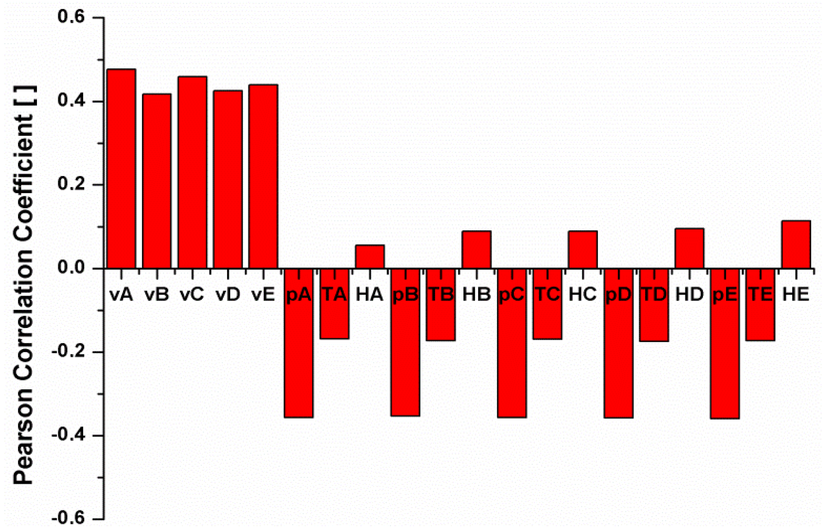
The hourly wind speed values predicted by the NWP for the five best-correlated sites, as previously described, considers the time horizon of the forecast. For example, when the forecast horizon is 1 h, the 5 predicted wind speeds for each site for the next hour in respect to the beginning of the forecast will be considered; for a prediction using a 24 h forecast horizon, the input vector includes the predicted values for the next 24 h for each site (120 forecasted wind speeds).

-

The numerical weather parameters (pressure, temperature and humidity) that are predicted hourly by the NWP, like the predicted wind speed.

For the wind power parameter P_m(i) the autocorrelation (ACF) and the partial autocorrelation (PAC) drastically decrease as the time lag increases, Lag 2 and 3 will not be considered because the PAC value is very close to the bounds of the 95% Confidence Interval of the PAC, as shown in Figure 1.

Figure 1. Autocorrelation function (a) and partial autocorrelation function (b) plots for the wind power P_m.

Figure 1. Autocorrelation function (a) and partial autocorrelation function (b) plots for the wind power P_m.

For the wind velocity and the weather parameters, Pearson’s correlation permits to determine which of these parameters are mostly related to the wind power and which should be considered. Figure 2 shows that the Pearson’s coefficient of the humidity for each site is lower than 0.09 that indicates no correlation with the wind power [42]. The wind velocity and the pressure are the variables that correlate the most to the wind power. A detailed sensitivity analysis on the input parameters was also carried out in [6] in order to find those numerical weather parameters with the best impact on the forecast by using the Artificial Neural Network trained with the different combinations of the weather parameters. In this study two input vectors were used to allow us to underline which method permits to better reduce the error due to low correlated input parameters, as the humidity. In the present work the input vector is in the general form:

xi = [v(A,i);… v(E,i) p(A,i)… p(E,i); T(A,i)… T(E,i); H(A,i)…H(E,i); P_m(i)]

(3)

In particular, two different input vectors were used (Table 1): the input vector I given by [v(A,i);… v(E,i) p(A,i)… p(E,i); T(A,i)… T(E,i); H(A,i)… H(E,i); P_m(i)] and the input vector II that does not take into account humidity and it is given by [v(A,i);… v(E,i) p(A,i)… p(E,i); T(A,i)…T(E,i); P_m(i)]. Table 2 shows, for the generic time horizon “i”, the Type “I” input vector.

Table 1. Numerical weather parameters included in the input vectors.

Input Vectors	Numerical Weather Parameters				Measured Data
	Site Speed vA, vB, vC, vD, vE	Pressure pA, pB, pC, pD, pE	Temperature TA, TB, TC, TD, TE	Humidity HA, HB, HC, HD, HE	Hourly average power Pm
I	X	X	X	X	X
II	X	X	X	-	X

Table 1. Numerical weather parameters included in the input vectors.

Input Vectors	Numerical Weather Parameters				Measured Data
	Site Speed vA, vB, vC, vD, vE	Pressure pA, pB, pC, pD, pE	Temperature TA, TB, TC, TD, TE	Humidity HA, HB, HC, HD, HE	Hourly average power Pm
I	X	X	X	X	X
II	X	X	X	-	X

Table 2. Input/target scheme for input vector I.

Horizon (Hours)	Input	Unit of Measurement	Target (kW)
L	vA, i+1 … vA, i+l vB, i+1 … vB, i+l vC, i+1 … vC, i+l vD, i+1 … vD, i+l vE, i+1 … vE, i+l	m/s	Pt+ 1 + …+ Pt +l
	pA, i+1 … pA, i+l pB, i+1 … pB, i+l pC, i+1 … pC, i+l pD, i+1 … pD, i+l pE, i+1 … pE, i+l	mmHg
	TA, i+1 … TA, i +l TB, i+1 … TB,i+l TC,i+1 … TC,i+l TD, i+1 … TD, i+l TE, i+1 … TE, i+l	°C
	HA, i+1 … HA, i+l HB,i+1 … HB, i+l HC, i+1 … HC, i+l HD, i+1 … HD, i+l HE, i+1 … HE, i+l	%
	Pmi	kW

Table 2. Input/target scheme for input vector I.

Horizon (Hours)	Input	Unit of Measurement	Target (kW)
L	vA, i+1 … vA, i+l vB, i+1 … vB, i+l vC, i+1 … vC, i+l vD, i+1 … vD, i+l vE, i+1 … vE, i+l	m/s	Pt+ 1 + …+ Pt +l
	pA, i+1 … pA, i+l pB, i+1 … pB, i+l pC, i+1 … pC, i+l pD, i+1 … pD, i+l pE, i+1 … pE, i+l	mmHg
	TA, i+1 … TA, i +l TB, i+1 … TB,i+l TC,i+1 … TC,i+l TD, i+1 … TD, i+l TE, i+1 … TE, i+l	°C
	HA, i+1 … HA, i+l HB,i+1 … HB, i+l HC, i+1 … HC, i+l HD, i+1 … HD, i+l HE, i+1 … HE, i+l	%
	Pmi	kW

Forecasting models were applied with a training period of 8 months and with a testing period of 4 months. The target used to evaluate model prediction is given by P_t(i,l), the sum of the hourly average powers P_m(r) during the forecast time horizon l, defined as:

(4)

To evaluate the forecasting performance, the predicted wind power values were compared with the measured ones. For this aim, several statistical metrics were introduced, which explained the average deviations between forecasted and measured data.

Figure 2. Pearson’s correlation coefficient for weather parameters.

Figure 2. Pearson’s correlation coefficient for weather parameters.

The accuracy of the predictions was evaluated considering the normalized mean absolute percentage error. Therefore the statistical metrics were considered as follows:

Normalized error E_i(l) = P_N(i,l) - T_N(i,l)

(5)

Normalized mean absolute error (%)

(6)

Normalized mean bias error

(7)

Root mean square error

(8)

where:

• i = generic hour of the predicted data;
• l = time horizon;
• M = number of predicted data, equal to 1896;
• , where T(i,l) is the predicted power at hour i for the time horizon l;
• , where P_t(i,l) is defined as Equation (4).

The RMSE (Root Mean Square Error) can be decomposed in three different terms: the bias, the SD_bias and the DISP (dispersion):

RMSE²(l) = bias²(l) + SD_bias²(l) + DISP²(l)

(9)

where SD_bias and DISP are the amplitude and the phase errors.

The amplitude error is due to an overestimation or underestimation of the measured data even if the prediction correctly describes the temporal evolution of the wind power. The phase error is due to a time shift of the predicted values in respect to the real data that occurs if the amplitude of the forecast is right, but arrives too early or too late.

The SD_bias and DISP are defined as follows:

Standard deviation bias SD_bias(1) = σ_T(l) − σ_P(l)

(10)

Dispersion

(11)

where:

• σ_T(l) = standard deviation of T_N(i,l)
• σ_P(l) = standard deviation of P_N(i,l)
• R_TP = the cross-correlation coefficient between T_N(i,l) and P_N(i,l)

4. The Least Squares Support Vector Machine Model

The LS-SVM method was introduced by [28], as a modified form of SVM of [27]. Given a training set of N data points , where x(I) is the i-th input data and P_t(i,l) is the i-th output data defined in Equation (4). The following regression model can be constructed by using , ϕ(x(i)) nonlinear function mapping of the input space to a higher dimensional space:

P_t(i,l) = wϕ(x(i)) + b₁, i = 1,…,N

(12)

where w is the weight vector and b₁ is the bias term.

To transform the above regression equation into a quadratic optimization problem with constraint is the equivalent to minimize a cost function. More details are reported in [28]. Radial Basis Function kernel RBF is used as the kernel function. The LS-SVM is tuned by searching the optimal regularization “kernel parameters” as well as the model order, using a 10-fold cross-validation (CV) procedure [28].

5. The Artificial Neural Network Method

An Elman ANN was implemented. This is a feed-forward network with a feedback connection from the first-layer output to the first layer input, thus enabling the detection and generation of time-varying patterns [7]. This characteristic is of great importance as the time-length of the prediction increases. The used scheme consists of three layers of neurons. The number of neurons in each layer is reported in Table 3. After an optimization process oriented to minimize the Mean Square Error, it was verified that for the hidden layer (layer 2) the best value corresponds to the mean of the neurons between the input and output layer [43]. In the first layer the hyperbolic tangent sigmoid transfer function (TANSIG) [44] was applied and in the second layer the linear transfer function (PURELIN) [45] was used.

The “gradient descent weight and bias” were used as learning function (LEARNGD) [46] to determine how to adjust the neuron weights to maximize performance.

Table 3. Elman network parameters used in the training process.

Number of layers		Input vector I	Input vector II
		3	3
Neurons (layer 1)	l = 1 h	21	16
	l = 3 h	31	26
	l = 6 h	61	51
	l = 12 h	121	101
	l = 24 h	241	201
Neurons (layer 2)	l = 1 h	11	8
	l = 3 h	16	13
	l = 6 h	31	26
	l = 12 h	61	51
	l = 24 h	121	101
Neurons (layer 3)—output		1	1

Table 3. Elman network parameters used in the training process.

Number of layers		Input vector I	Input vector II
		3	3
Neurons (layer 1)	l = 1 h	21	16
	l = 3 h	31	26
	l = 6 h	61	51
	l = 12 h	121	101
	l = 24 h	241	201
Neurons (layer 2)	l = 1 h	11	8
	l = 3 h	16	13
	l = 6 h	31	26
	l = 12 h	61	51
	l = 24 h	121	101
Neurons (layer 3)—output		1	1

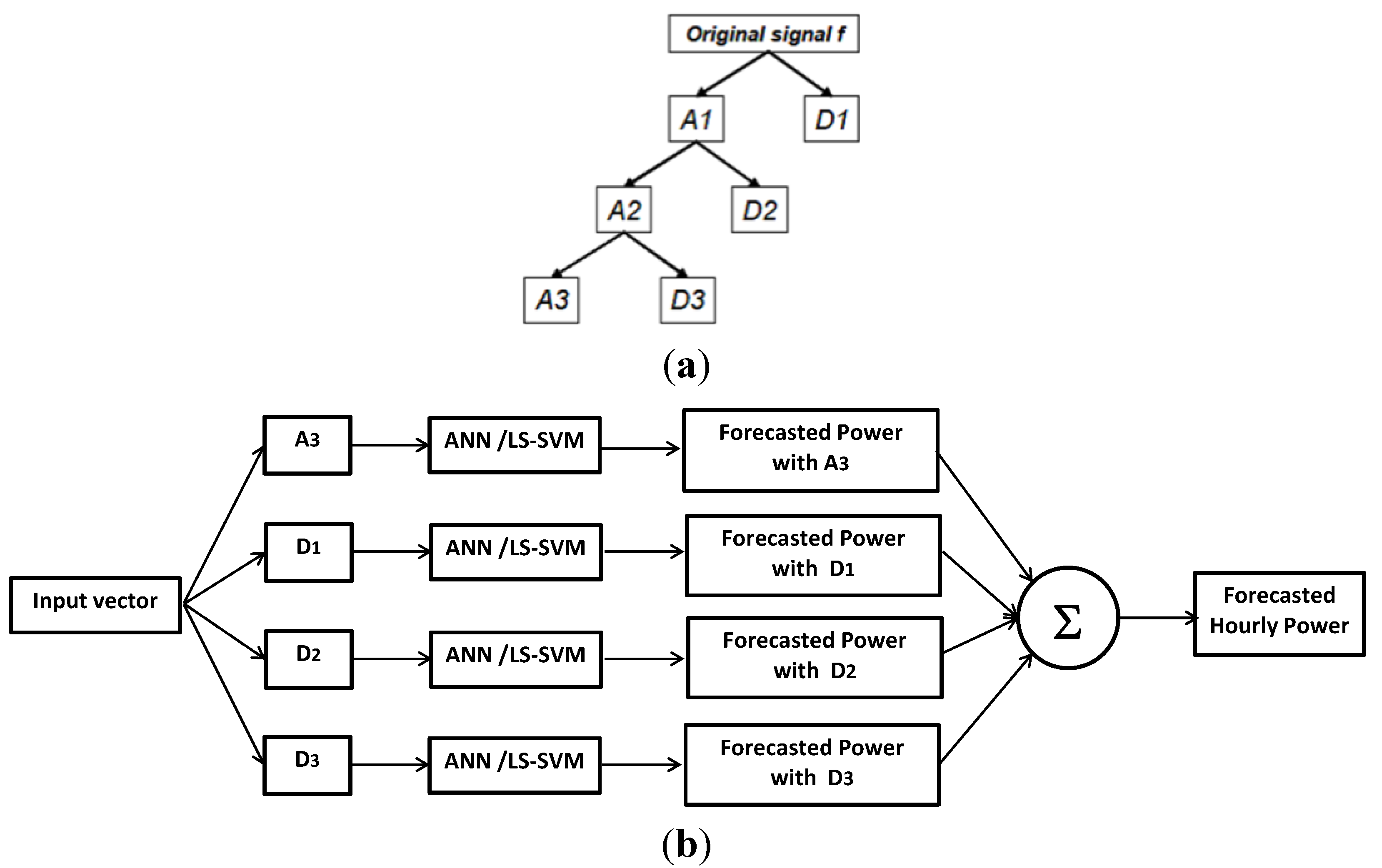
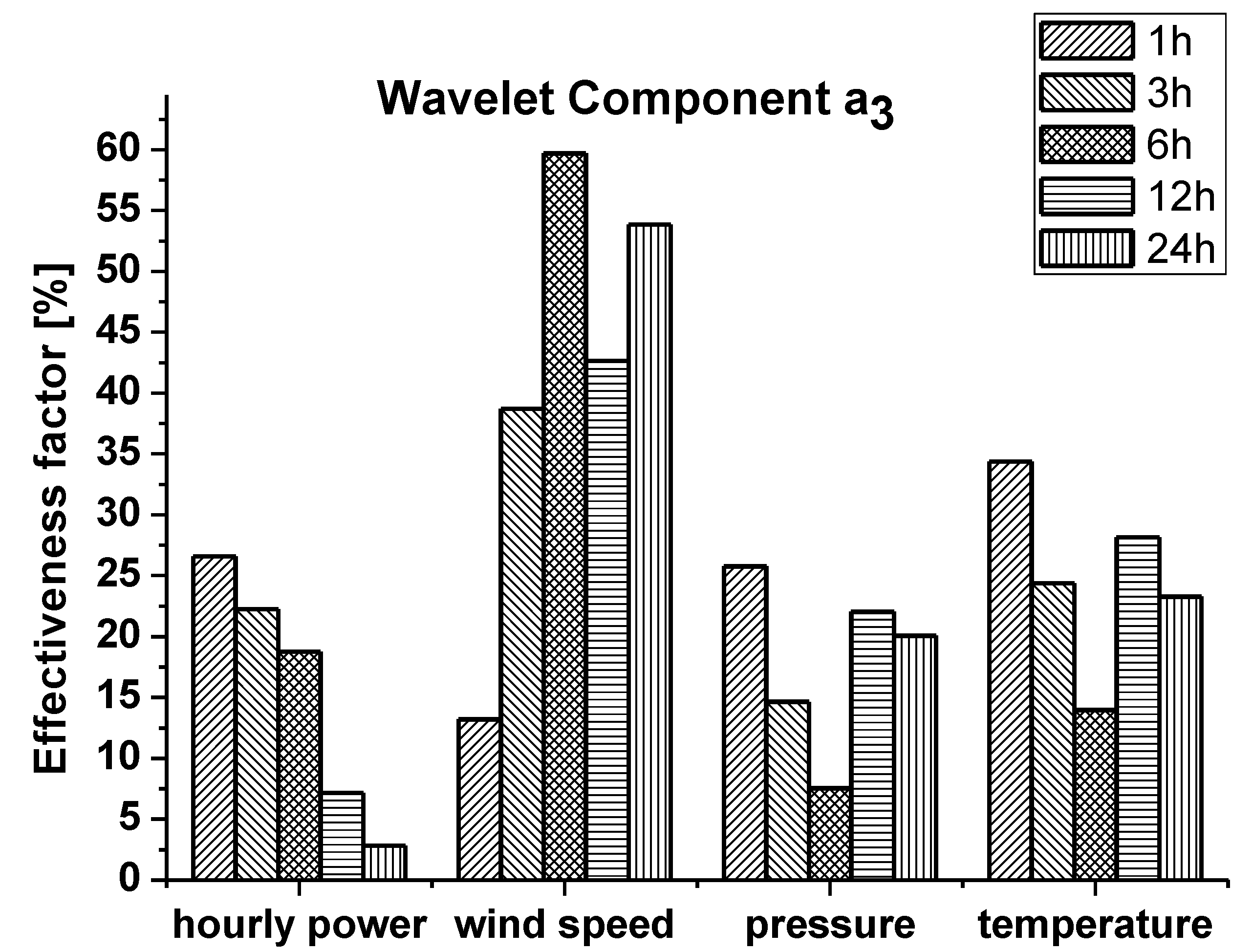
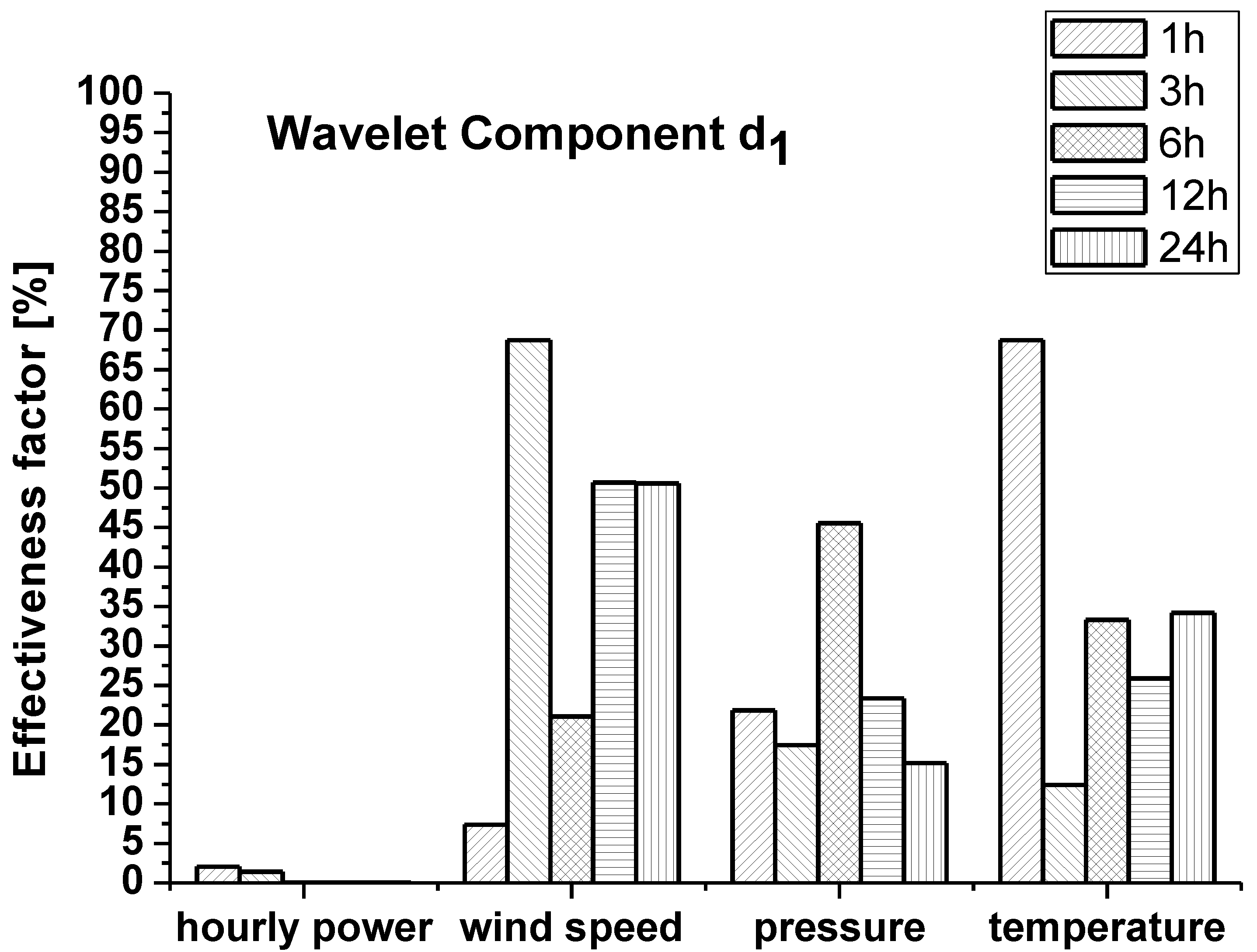
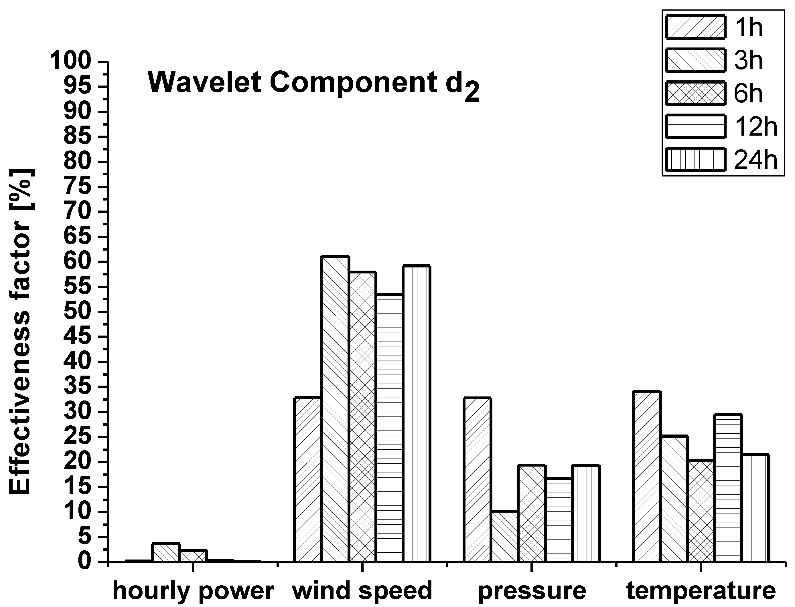
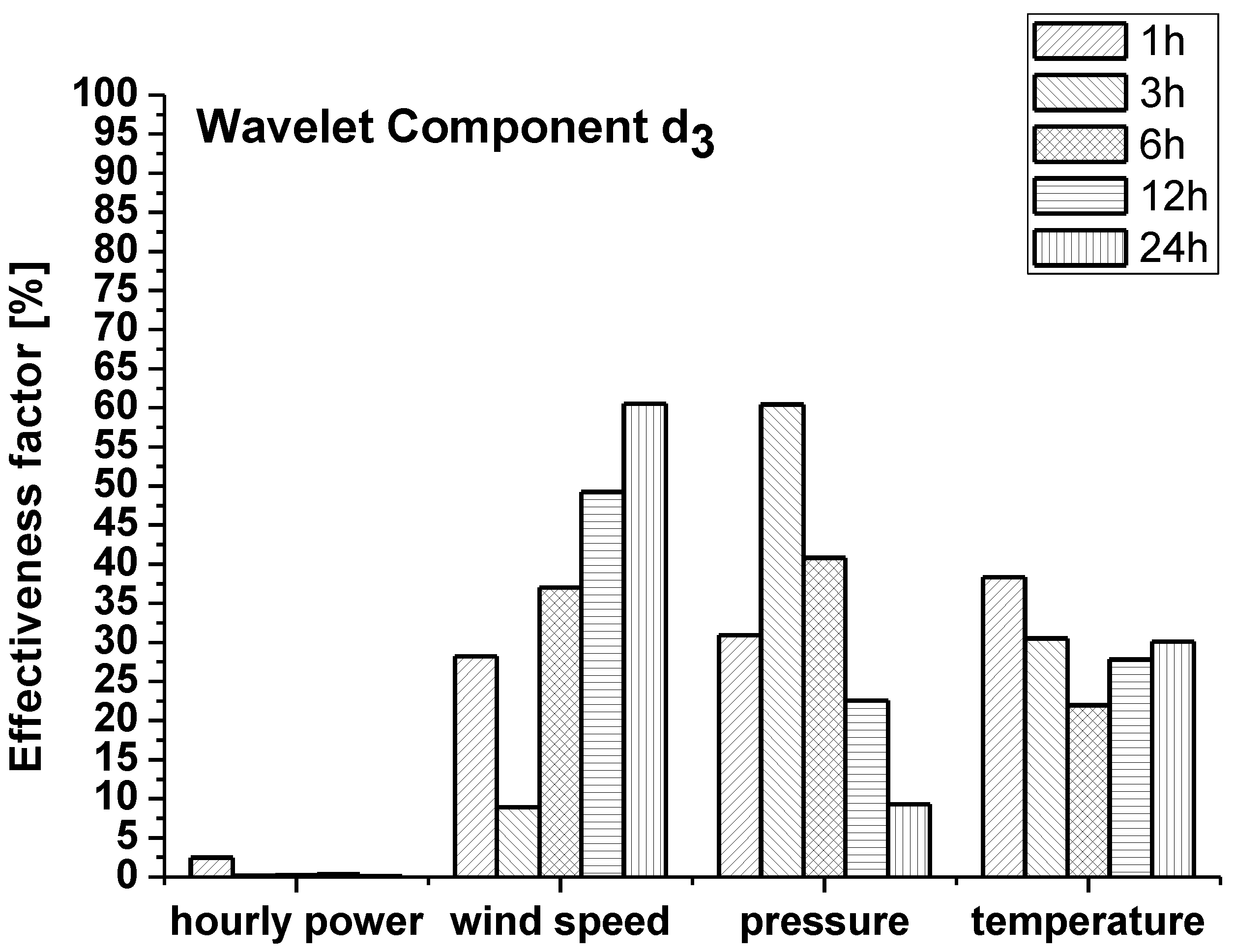
6. Wavelet Decomposition Technique

The time series of wind speed, temperature and pressure data include information on daily, seasonal and long-term behaviors; to improve the forecasting model performance, it should be suitable to use the original data fitted into predetermined frequency (or time period) bands. For this purpose, the forecasting models can be based on the Wavelet decomposition (WD) of the input data.

In the proposed method, a fast Discrete Wavelet Transform (DWT) algorithm developed by Mallat [24] and based on decomposition and reconstruction, low-pass and high-pass filters were used. This algorithm obtains “approximations” and “details” from a given signal. An approximation is a low-frequency representation of the original signal, whereas a detail is the difference between two successive approximations and depicts high-frequency components of the signal.

In the present work, a Daubechies Wavelet of order 6th (abbreviated by D_b6) is used as the mother wavelet. Three levels of decomposition were used. The corresponding frequency (time period) band for the approximation level is 0–0.0625 [1/h], and for the detail levels d₁, d₂, d₃ the bands are respectively: 0.25–0.5 [1/h]; 0.125–0.25 [1/h]; 0.0625–0.125 [1/h].

The training of ANN and LS-SVM were done for each of the four WD components, and then an aggregation of the four partial forecast results was performed for the final prediction of wind power.

Then ANN and LS-SVM with WD was performed carrying out the following sequence (Figure 3):

-

Six Daubechies Wavelet Decomposition employed to carry out the 3rd level discrete WD of the original hourly time series; the approximation component A₃ and the three detail components D₁, D₂ and D₃ were obtained.

-

Training of the forecast model (ANN or LS-SVM), one for each of the four WD components.

-

Aggregation of the four partial forecast results for final predicted wind power.

Figure 3. (a) Multilevel decomposition process: A and D stand for approximation and detail, respectively (f = A₃ + D₁ + D₂ + D₃); (b) Architecture of the forecast system.

Figure 3. (a) Multilevel decomposition process: A and D stand for approximation and detail, respectively (f = A₃ + D₁ + D₂ + D₃); (b) Architecture of the forecast system.

7. Results

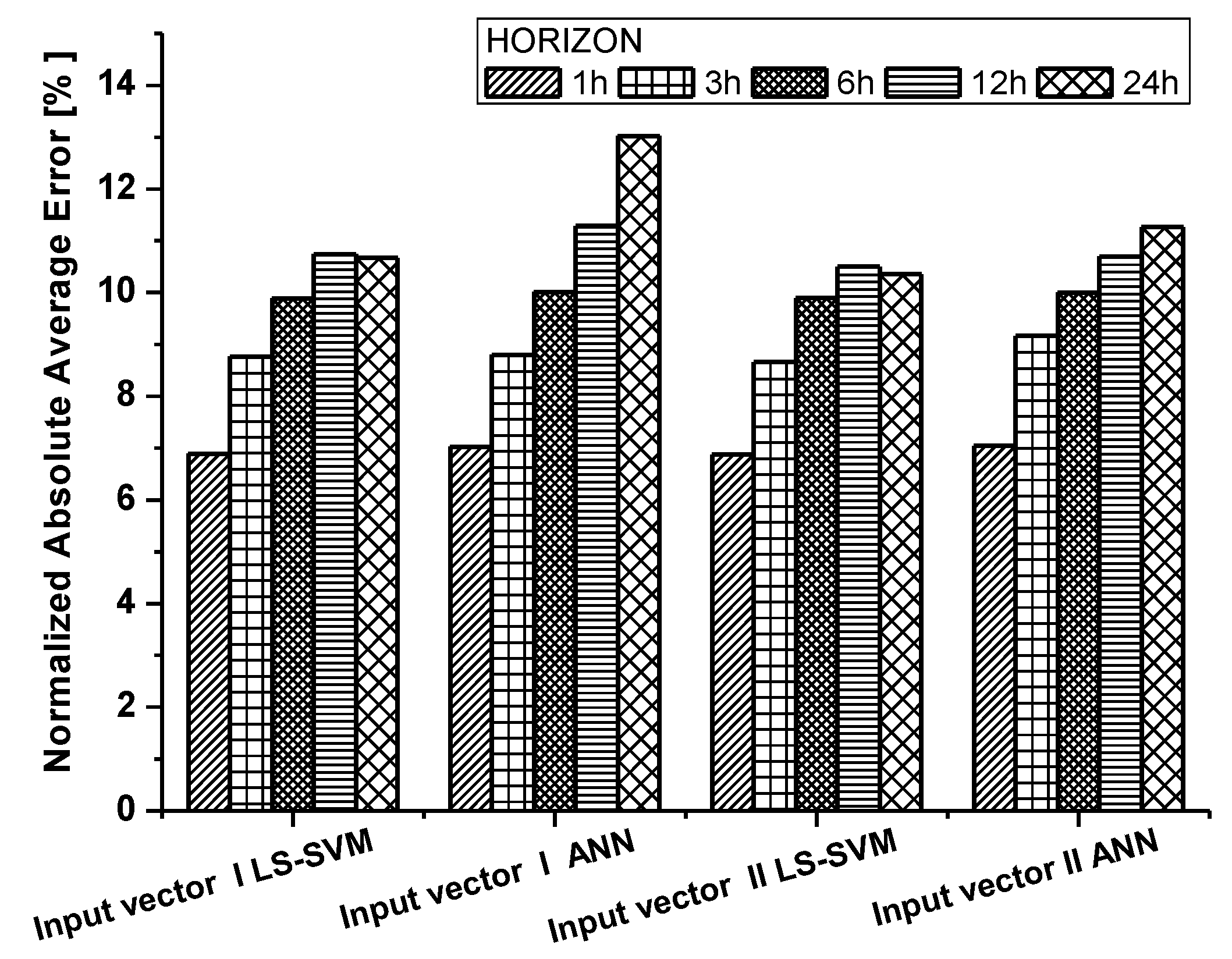
7.1. Forecasting Based on Artificial Neural Networks and LS-SVM

The ANN model was first applied to the original data without Wavelet Decomposition. As previously seen, the forecasting model was implemented with a training period of 8 months and with a testing period of 4 months. In Figure 4, the NMAE (Normalized Mean Absolute Error) values for the two input vectors are summarized. The results show that, besides the obvious importance of wind speed, the NWP data that positively impact the predictions are pressure and temperature. Including relative humidity data in the input variables (input vector of Type I) leads to a higher NMAE value compared to the case of input vector Type II, which considers a prediction based only on predicted wind speeds, pressures and temperatures, except for the horizon of 3-h. This behavior is more evident in the two long time periods used for prediction (12-h, 24-h). As shown in Figure 4 and Table 4, LS-SVM improves the performances using both the input datasets (input Types I and II).

Focusing on the two input types and both methods, the use of the LS-SVM method mostly permits to reduce the error due to the presence of the uncorrelated variable, the humidity. Furthermore the use of input data Type II gives better predictions also in the case of LS-SVM in terms of NMAE(l) and E(i,l) distribution, in particular, at long time periods of forecasting. The longer time interval prediction leads to larger prediction error, due to uncorrelated data; it is clear that it is preferable to eliminate the humidity data from the input dataset. For 24-h forecasting, and for input data of Type I, more than 63% predicted points show normalized errors E_i less than 10%. For input data of Type I, the same error level was shown by approximately 60% of the predicted points. For shorter time periods of forecasting, the prediction errors and its probability distribution are quite similar.

Figure 4. Histogram of NMAE for input vector Type I and Type II by LS-SVM and ANN.

Figure 4. Histogram of NMAE for input vector Type I and Type II by LS-SVM and ANN.

Table 4. NMAE and Error Range Probability for input vector Type I and Type II by LS-SVM prediction model.

Time Horizon	Normalized Absolute Average Error	Error Range Probability [−10%; +10%]	Error Range Probability [−20%; +20%]	Prediction Length	Normalized Absolute Average Error	Error Range Probability [−10%; +10%]
	Input vector I LS-SVM	Input vector II LS-SVM	Input vector I LS-SVM	Input vector II LS-SVM	Input vector I LS-SVM	Input vector II LS-SVM
1 h	6.89%	6.88%	78.36%	78.29%	91.83%	91.76%
3 h	8.76%	8.67%	70.50%	70.67%	88.40%	88.51%
6 h	9.90%	9.89%	66.11%	64.94%	85.78%	85.65%
12 h	10.74%	10.51%	63.27%	63.31%	82.95%	84.40%
24 h	10.67%	10.36%	59.73%	63.34%	86.16%	86.65%

Table 4. NMAE and Error Range Probability for input vector Type I and Type II by LS-SVM prediction model.

Time Horizon	Normalized Absolute Average Error	Error Range Probability [−10%; +10%]	Error Range Probability [−20%; +20%]	Prediction Length	Normalized Absolute Average Error	Error Range Probability [−10%; +10%]
	Input vector I LS-SVM	Input vector II LS-SVM	Input vector I LS-SVM	Input vector II LS-SVM	Input vector I LS-SVM	Input vector II LS-SVM
1 h	6.89%	6.88%	78.36%	78.29%	91.83%	91.76%
3 h	8.76%	8.67%	70.50%	70.67%	88.40%	88.51%
6 h	9.90%	9.89%	66.11%	64.94%	85.78%	85.65%
12 h	10.74%	10.51%	63.27%	63.31%	82.95%	84.40%
24 h	10.67%	10.36%	59.73%	63.34%	86.16%	86.65%

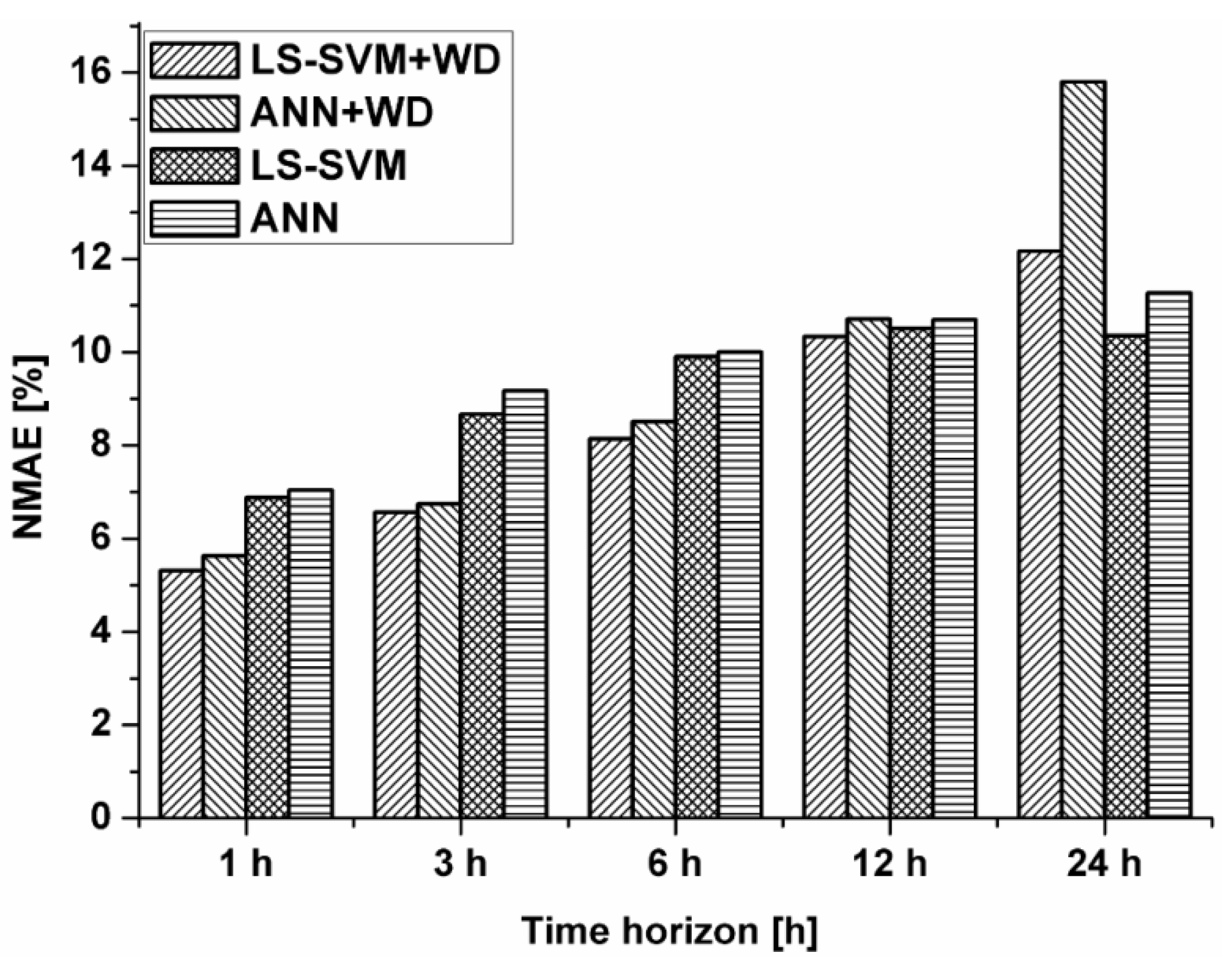
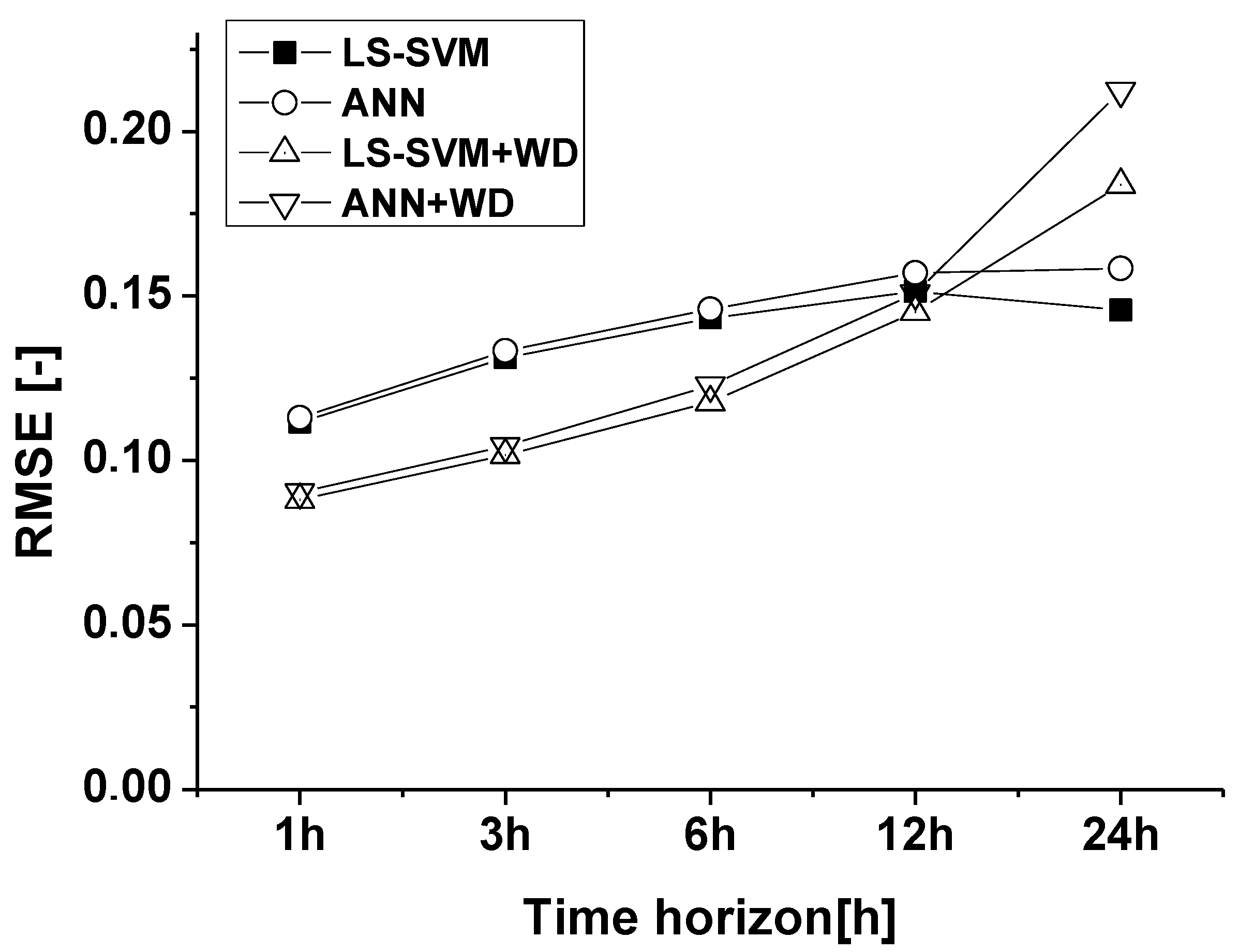
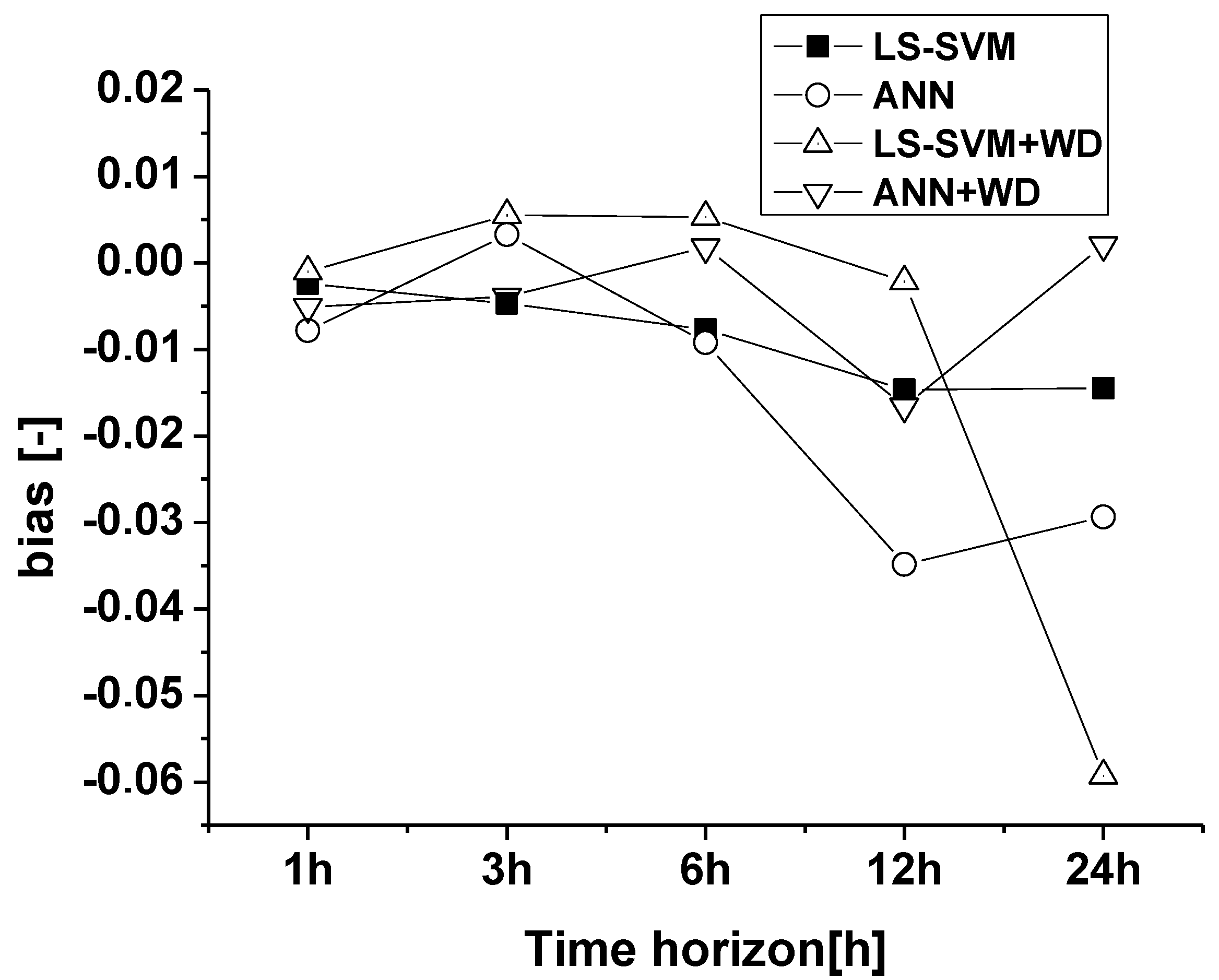
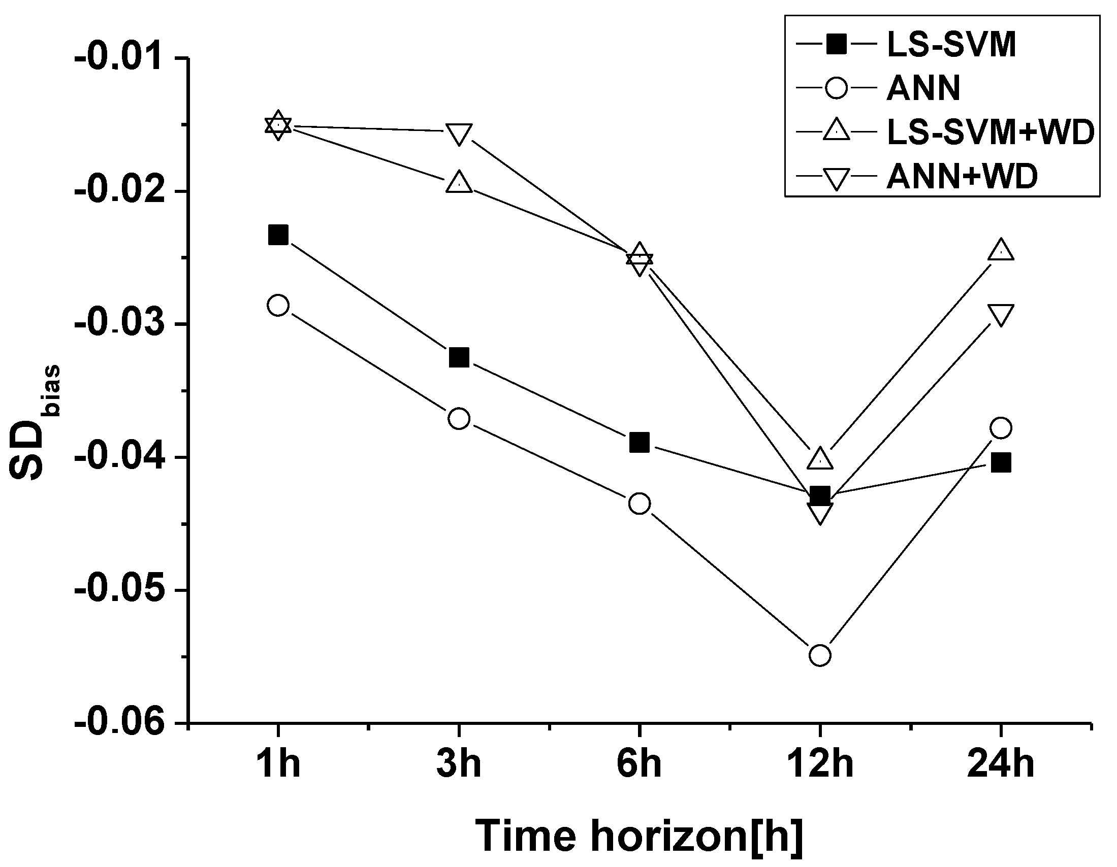
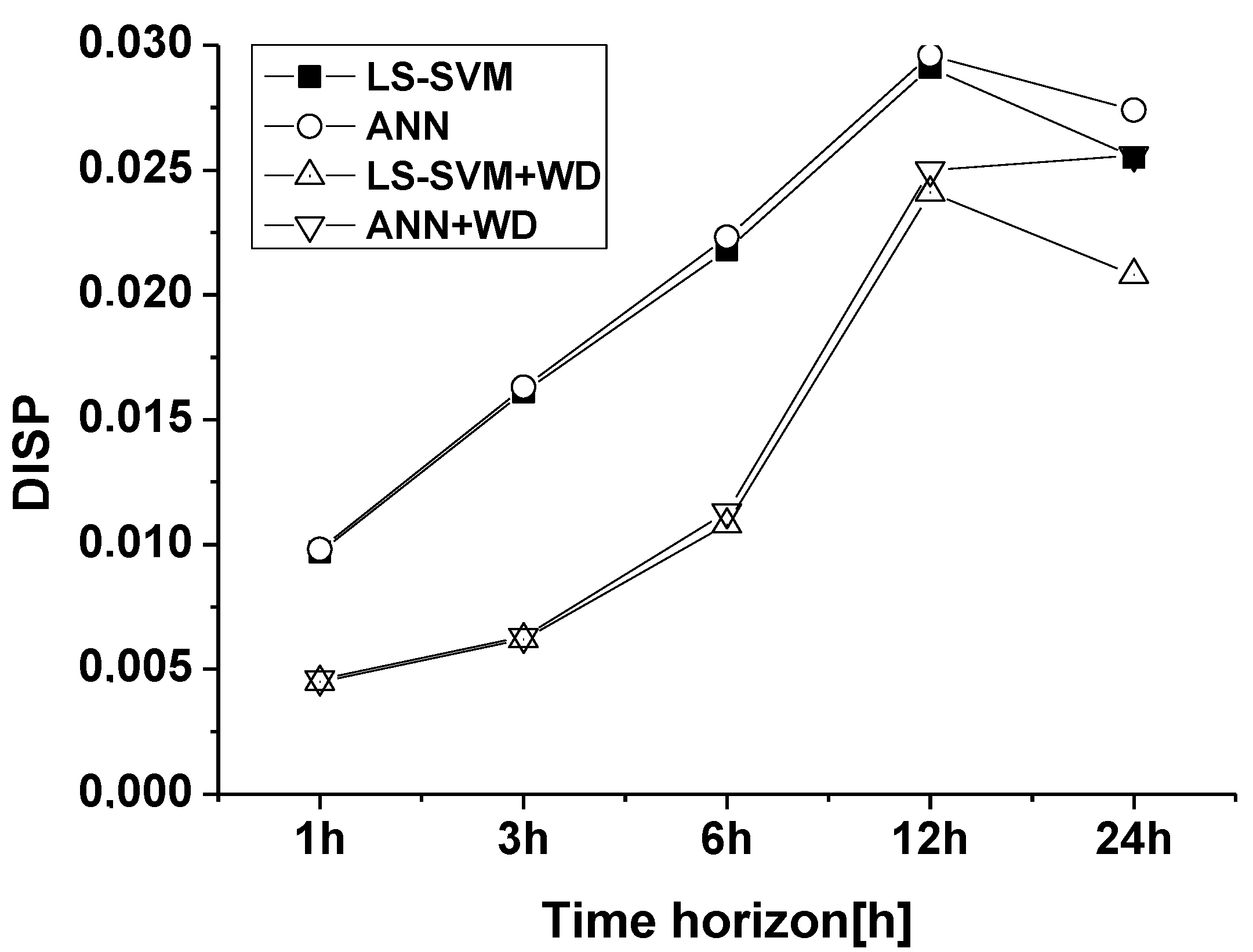
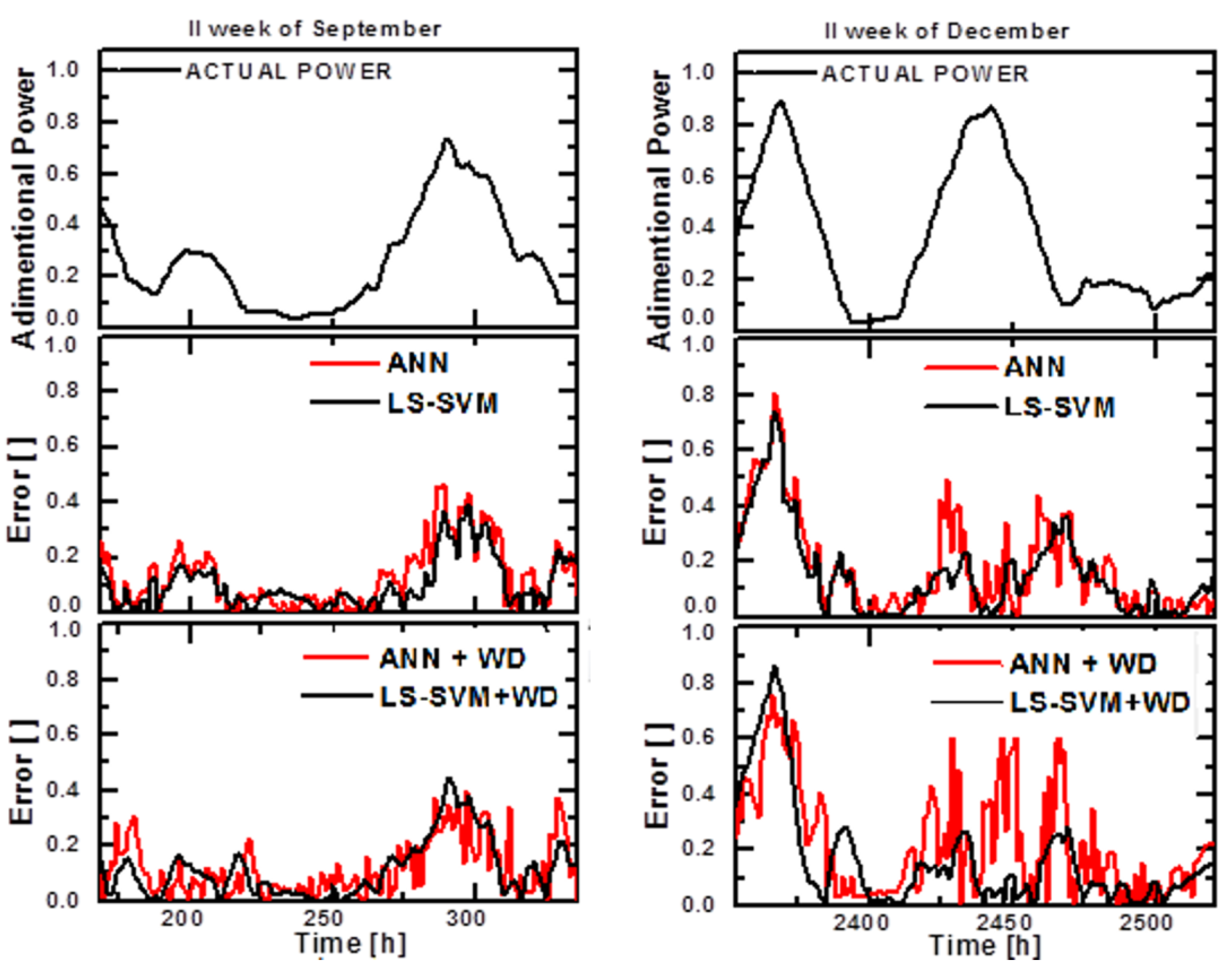
7.2. Wind Power Forecast by Wavelet Based Forecasting Methods

The proposed algorithm was applied to datasets of input vector Type II (Table 1). The hybridization of LS-SVM by WD was investigated and the results compared with similar results of the hybridized ANN. Focusing to the input vector Type II, the comparisons between NMAE values with and without WD are given in Table 5. In the same table the probability that an error E(i,l) occurs in the range ±10% or ±20% is reported. It’s evident the benefit due to WD at short-medium prediction horizons. However, the WD approach, essentially statistical, tends to be more computationally expensive, especially when the forecast time period becomes longer.

As shown in Figure 5 for short term prediction (from 1-h up to 6-h ahead forecasting) hybrid methods based on WD lead to better results for both ANN and LS-SVM, with slightly better accuracy for LS-SVM. LS-SVM approach without WD outperforms other approaches at long term (24-h).

This is also confirmed by the RMSE in Figure 6. RMSE gives more weight to large errors, whereas NMAE reveals the average magnitude of the error and bias (Figure 7) and it indicates whether there is a significant (and corrigible) tendency to systematically over-forecast or under-forecast.

Table 5. NMAE and Error Range Probability for input vector Type II by LS-SVM and ANN without and with WD.

Normalized Absolute Average Error NMAE
Time Horizon	Input Vector IIANN	Input Vector IILS-SVM	Input Vector IIANN with WD	Input Vector IILS-SVM with WD
1 h	7.04%	6.88%	5.67%	5.31%
3 h	9.17%	8.67%	6.83%	6.57%
6 h	9.99%	9.89%	8.56%	8.14%
12 h	10.70%	10.51%	10.92%	10.33%
24 h	11.27%	10.36%	15.50%	12.16%
Error Range Probability [−10%; +10%]
Time Horizon	Input vector IIANN	Input vector IILS-SVM	Input vector IIANN with WD	Input vector IILS-SVM with WD
1 h	78.19%	78.29%	82.84%	83.56%
3 h	71.88%	70.50%	78.12%	78.15%
6 h	67.43%	64.94%	71.61%	71.62%
12 h	65.11%	63.27%	60.95%	64.02%
24 h	59.56%	63.34%	43.42%	56.65%
Error Range Probability [−20%; +20%]
Time Horizon	Input Vector IIANN	Input Vector IILS-SVM	Input Vector IIANN with WD	Input Vector IILS-SVM with WD
1 h	91.45%	91.76%	94.93%	95.07%
3 h	88.68%	88.51%	92.17%	92.18%
6 h	85.55%	85.65%	88.66%	89.63%
12 h	82.43%	84.40%	83.96%	84.80%
24 h	84.35%	86.65%	72.44%	81.36%

Table 5. NMAE and Error Range Probability for input vector Type II by LS-SVM and ANN without and with WD.

Normalized Absolute Average Error NMAE
Time Horizon	Input Vector IIANN	Input Vector IILS-SVM	Input Vector IIANN with WD	Input Vector IILS-SVM with WD
1 h	7.04%	6.88%	5.67%	5.31%
3 h	9.17%	8.67%	6.83%	6.57%
6 h	9.99%	9.89%	8.56%	8.14%
12 h	10.70%	10.51%	10.92%	10.33%
24 h	11.27%	10.36%	15.50%	12.16%
Error Range Probability [−10%; +10%]
Time Horizon	Input vector IIANN	Input vector IILS-SVM	Input vector IIANN with WD	Input vector IILS-SVM with WD
1 h	78.19%	78.29%	82.84%	83.56%
3 h	71.88%	70.50%	78.12%	78.15%
6 h	67.43%	64.94%	71.61%	71.62%
12 h	65.11%	63.27%	60.95%	64.02%
24 h	59.56%	63.34%	43.42%	56.65%
Error Range Probability [−20%; +20%]
Time Horizon	Input Vector IIANN	Input Vector IILS-SVM	Input Vector IIANN with WD	Input Vector IILS-SVM with WD
1 h	91.45%	91.76%	94.93%	95.07%
3 h	88.68%	88.51%	92.17%	92.18%
6 h	85.55%	85.65%	88.66%	89.63%
12 h	82.43%	84.40%	83.96%	84.80%
24 h	84.35%	86.65%	72.44%	81.36%

Figure 5. Histogram of NMAE for input vector Type II by LS-SVM and ANN without and with WD.

Figure 5. Histogram of NMAE for input vector Type II by LS-SVM and ANN without and with WD.

Figure 6. RMSE for input vector Type II by LS-SVM and ANN without and with WD.

Figure 6. RMSE for input vector Type II by LS-SVM and ANN without and with WD.

Figure 7. Bias error for input vector Type II by LS-SVM and ANN without and with WD.

Figure 7. Bias error for input vector Type II by LS-SVM and ANN without and with WD.

The decomposition of the RMSE into three contributions provides a better understanding of the origin of the differences between prediction and measurement. Furthermore, recent power forecasting systems typically take into account systematic errors by estimating the forecast bias (bias) and the SD_bias error and then applying statistical correction schemes prior to analysis. The bias can be subtracted and increasing or decreasing the standard deviation of the prediction, contrary to the phase error, can adjust the SD_bias. Phase deviations reflect the time accuracy of the prediction model and constitute the challenge for further improvements. The DISP provides a lower limit to the RMSE; therefore forecasting methods with low DISP allow for a better accuracy. As shown in Figure 8, the SD_bias assumes negative values. It is consistent with findings in [47], in which it is underlined that the sites in flat terrain present positive bias and small SD_bias, while the sites with complex terrain present negative bias and large SD_bias at almost all prediction times.

Figure 8. SD_bias for input vector Type II by LS-SVM and ANN without and with WD.

Figure 8. SD_bias for input vector Type II by LS-SVM and ANN without and with WD.

Regarding relative dispersion in Figure 9, the different methods ANN and LS-SVM are rather similar.

For the methods without WD, the DISP is in a rather narrow range of increasing linearly with the forecast horizon, from 1-h up to 12-h. A spread is evident among the methods without and with WD. The reduction in the phase error (DISP) is mainly due to the implementation of the Wavelet Decomposition rather than the choice of LS-SVM or ANN. Even if the use of LS-SVM allows a further decrease at the phase error 24-h.

Forecast accuracy depends on the particular month under examination. The difference of forecasting accuracy can be correlated with temporal variation of NWP data as wind speed, temperature and pressure; the variation is estimated for each variable as the ratio between the absolute difference of two consecutive hourly values and the mean of values in the test period.

Figure 9. DISP for input vector Type II by LS-SVM and ANN without and with WD.

Figure 9. DISP for input vector Type II by LS-SVM and ANN without and with WD.

Comparing forecast errors in Figure 10 and the temporal variability of NWP data shown in Figure 11, it is evident that temporal variability is generally higher in December than in September and the greater and more irregular the wind speed is, the worse the resulting forecasting precision, in particular for methods based on ANN. Prediction errors are more influenced by wind speed dynamic variation than absolute magnitude of wind speed or other NWP data.

Figure 10. Error Ei and actual wind power in two different weeks of year.

Figure 10. Error Ei and actual wind power in two different weeks of year.

Figure 11. Temporal variability of NWP data in two different weeks of year.

Figure 11. Temporal variability of NWP data in two different weeks of year.

A sensitivity analysis, for a deeper understanding of these results, was performed on each component of the WD decomposition to analyze the effect of the training parameters on the model predictions.

For this purpose, an effectiveness factor α_j was defined to show the influence of each input x_i(j) representing the q adopted input parameters on model output [31,32,33]. Given defined as:

Root mean square error

(13)

T(i,l) is the output of the neural network model with the input x(i) defined in Equation (3) and T_j(i,l) is the output of the neural network model with the input x(i,j) = [ ], where is the average of xj(i) over the total number of samples M and it is given by:

Root mean square error

(14)

The effectiveness factor αj is defined as:

Root mean square error

(15)

where q is the total number of inputs.

The results of the effectiveness factor for each variable, averaged for all five sites, are shown in Figure 12, Figure 13, Figure 14 and Figure 15. For the component a₃ all input variables show the same behavior, in accordance with its characteristic to hold a generic trend of the original signal. A negligible influence of the measured power produced on ANN training is evident for the detail components, while NWP time series assume higher significant values, compared to a₃ behavior, for short and very short prediction time lengths: in particular, the temperature for the component d₁ and the pressure for the component d₃, will exert a significant influence on the training of the ANN.

Figure 12. Histogram of the effectiveness factors for the approximation component a₃.

Figure 12. Histogram of the effectiveness factors for the approximation component a₃.

The analysis confirms the importance of the application of the wavelet decomposition that allows the input parameters with high frequency contents, such as the NWP temperature, to have a more significant influence on the training of ANN for the detail component d₁. While the input parameters with low frequency component, such as NWP pressure, will exert a more significant influence on the training of ANN for the detail component d₃. It is consistent with the findings that were reported by the authors in [6], the FFT amplitude of pressure data has a high contribution in the frequency band 0.0625–0.125 [1/h] that corresponds to the scale d₃ of the WD.

Figure 13. Histogram of the effectiveness factors for the detail component d₁.

Figure 13. Histogram of the effectiveness factors for the detail component d₁.

Figure 14. Histogram of the effectiveness factors for the detail component d₂.

Figure 14. Histogram of the effectiveness factors for the detail component d₂.

Figure 15. Histogram of the effectiveness factors for the detail component d₃.

Figure 15. Histogram of the effectiveness factors for the detail component d₃.

8. Discussion and Conclusions

In this study, a novel hybrid method based on LS-SVM algorithm and WD of input signals, was compared with hybrid methods based on ANN. It is found that methods based on LS-SVM perform better than ANN for all the horizons. In particular, at a short time horizon an improvement of LS SVM performances is due the application of WD, while the simple LS-SVM without WD outperforms other methods at 24-h head forecasting.

The decomposition of the root mean squared error into three contributions (bias, standard deviation bias and dispersion) provides a better understanding of the origin of the differences between prediction and measurement. The bias can be subtracted and increasing or decreasing the standard deviation of the prediction, contrary to the dispersion error, can adjust the standard deviation. Therefore, the reduction of the dispersion error constitutes the challenge for further improvements; hence forecasting methods with low DISP allows improvement in accuracy. The analysis showed that the reduction in the dispersion is mainly due to the implementation of the Wavelet Decomposition rather than the choice of the LS-SVM or ANN, even if the use of LS-SVM allows for a further decrease of the phase error at 24h.

Comparing forecast errors for all the non-linear statistical approaches and the temporal variability of NWP data it is evident that the greater and more irregular the wind speed is, the worse the resulting forecasting precision, in particular for methods based on ANN. Therefore prediction accuracy is influenced by wind speed dynamic variation more than by the absolute magnitude of NWP data. The LS-SVM model detects better the properties of the wind speed time series when used in the training process.

LS-SVM solves a set of only linear equations, which is much easier and computationally simpler than SVM or ANN. At the same time, over-fitting is hard to find in the case of LS-SVM, while it is a disadvantage of ANN. LS-SVM could be a good alternative to the well-known ANNs, since it achieves better precision, good generalization capability and smaller computational time for training.

Then LS-SVM presents less parameters to optimize (regularization parameter, RBF kernel parameter and the number of previous data) than ANN, which requires optimization of the number of hidden layers, hidden nodes, and transfer functions.

Finally, LS-SVM requires small sample size, because the determination of the decision function is only due to the supporting vectors that are a part of a training pattern whilst remaining patterns are not used. On the contrary, ANN uses all training data sets. This feature, together with the error minimization approach, leads to a higher generalization of the relationship between past data and future power values for LS-SVM and more suitable for long term prediction.

The study also underlines that the use of an input vector with all the parameters available doesn’t entail the minimum prediction error. A comparison between forecasting systems with different input datasets was also carried out. Firstly, a multiple regression analysis was used to estimate the influence of input datasets. The analysis shows a good correlation with wind power for the set inputs given by wind speed, pressure and temperature.

A further sensitivity analysis based on an effectiveness factor was performed for the hybrid ANN with WD. The sensitivity analysis applied to each component highlights the high frequency content of the temperature and pressure data.

The results show that the NWP time series assume higher values of effectiveness factor for short and very short prediction lengths: in particular temperature for the component d₁ that corresponds to high frequency 0.25–0.5 [1/h] and pressure for the component d₃, frequency band 0.0625–0.125 [l/h]. The analysis also confirms the importance of the decomposition, which provides the input parameter with high frequency content, such as temperature, to have more weight in the training of ANN based on d₁ detail component and the input parameter with low frequency component, such as pressure, to contribute more to the training of ANN based on detail component d₃.

References

1. Congedo, P.M.; Malvoni, M.; Mele, M.; de Giorgi, M.G. Performance measurements of monocrystalline silicon PV modules in South-eastern Italy. Energy Convers. Manag. 2013, 68, 1–10. [Google Scholar] [CrossRef]
2. Wu, J.; Wang, J.; Lu, H.; Dong, Y.; Lu, X. Short term load forecasting technique based on the seasonal exponential adjustment method and the regression model. Energy Convers. Manag. 2013, 70, 1–9. [Google Scholar] [CrossRef]
3. Xydis, G.; Koroneos, C.; Loizidou, M. Exergy analysis in a wind speed prognostic model as a wind farm sitting selection tool: A case study in Southern Greece. Appl. Energy 2009, 86, 2411–2420. [Google Scholar] [CrossRef]
4. Foley, A.M.; Leahy, P.G.; Marvuglia, A.; McKeogh, E.J. Current methods and advances in forecasting of wind power generation. Renew. Energy 2012, 37, 1–8. [Google Scholar] [CrossRef] [Green Version]
5. De Giorgi, M.G.; Ficarella, A.; Russo, M.G. Short-term wind forecasting using artificial neural networks (ANNs). WIT Trans. Ecol. Environ. 2009, 121, 197–208. [Google Scholar] [CrossRef]
6. De Giorgi, M.G.; Ficarella, A.; Tarantino, M. Assessment of the benefits of numerical weather predictions in wind power forecasting based on statistical methods. Energy 2011, 36, 3968–3978. [Google Scholar] [CrossRef]
7. De Giorgi, M.G.; Ficarella, A.; Tarantino, M. Error analysis of short term wind power prediction models. Appl. Energy 2011, 88, 1298–1311. [Google Scholar] [CrossRef]
8. De Giorgi, M.G.; Tarantino, M.; Ficarella, A. Comparisons of different wind power forecasting systems. In Proceedings of the ASME 2010 10th Biennial Conference on Engineering Systems Design and Analysis, Istanbul, Turkey, 12–14 July 2010; pp. 105–113.
9. Flores, A.T.; Tapia, G. Application of a control algorithm for wind speed prediction and active power generation. Renew. Energy 2005, 33, 523–536. [Google Scholar] [CrossRef]
10. Beccali, M.; Cirrincione, G.; Marvuglia, A.; Serporta, C. Estimation of wind velocity over a complex terrain using the Generalized Mapping Regressor. Appl. Energy 2010, 87, 884–893. [Google Scholar] [CrossRef] [Green Version]
11. Cadenas, E.; Rivera, W. Wind speed forecasting in the South Coast of Oaxaca, Mexico. Renew. Energy 2006, 32, 2116–2128. [Google Scholar] [CrossRef]
12. Li, G.; Shi, J. On comparing three artificial neural networks for wind speed forecasting. Appl. Energy 2010, 87, 2313–2320. [Google Scholar] [CrossRef]
13. Sfetsos, A. A novel approach for the forecasting of mean hourly wind speed time series. Renew. Energy 2002, 27, 163–174. [Google Scholar] [CrossRef]
14. Sideratos, G.; Hatziargyriou, N.D. Probabilistic wind power forecasting using radial basis function neural networks. IEEE Trans. Power Syst. 2012, 27, 1788–1796. [Google Scholar] [CrossRef]
15. Khosravi, A.; Nahavandi, S.; Creighton, D.; Atiya, A.F. Comprehensive review of neural network-based prediction intervals and new advances. IEEE Trans. Neural Netw. 2011, 22, 1341–1356. [Google Scholar] [CrossRef]
16. Taylor, J.W.; Buizza, R. Neural network load forecasting with weather ensemble predictions. IEEE Trans. Power Syst. 2002, 17, 626–632. [Google Scholar] [CrossRef]
17. Quan, H.; Srinivasan, D.; Khosravi, A. Short-term load and wind power forecasting using neural network-based prediction intervals. IEEE Trans. Neural Netw. Learn. Syst. 2014, 25, 303–315. [Google Scholar] [CrossRef]
18. Hippert, H.; Pedreira, C.; Souza, R. Neural networks for short-term load forecasting: A review and evaluation. IEEE Trans. Power Syst. 2001, 16, 44–55. [Google Scholar] [CrossRef]
19. Hong, Y.-Y.; Yu, T.-H.; Liu, C.-Y. Hour-ahead wind speed and power forecasting using empirical mode decomposition. Energies 2013, 6, 6137–6152. [Google Scholar] [CrossRef]
20. Sideratos, G.; Hatziargyriou, N.D. An advanced statistical method for wind power forecasting. IEEE Trans. Power Syst. 2007, 22, 258–265. [Google Scholar] [CrossRef]
21. Chang, W.-Y. Short-term wind power forecasting using the enhanced particle swarm optimization based hybrid method. Energies 2013, 6, 4879–4896. [Google Scholar] [CrossRef]
22. Guan, C.; Luh, P.; Michel, L.; Chi, Z. Hybrid Kalman filters for very short-term load forecasting and prediction interval estimation. IEEE Trans. Power Syst. 2013, 28, 3806–3817. [Google Scholar] [CrossRef]
23. De Giorgi, M.G.; Tarantino, M.; Ficarella, A. A new hybrid method for wind power forecasting based on wavelet decomposition and artificial neural networks. In Proceedings of the ASME Turbo Expo, Turbine Technical Conference and Exposition, GT2011, Vancouver, BC, Canada, 6–10 June 2011; pp. 889–900.
24. Mallat, S. A theory for multiresolution signal decomposition and wavelet representation. IEEE Trans. Pattern Anal. Mach. Intell. 1989, 11, 674–693. [Google Scholar] [CrossRef]
25. An, X.; Jiang, D.; Liu, C.; Zhao, M. Wind farm power prediction based on wavelet decomposition and chaotic time series. Expert Syst. Appl. 2011, 38, 11280–11285. [Google Scholar] [CrossRef]
26. Amjady, N.; Keynia, F. Short-term load forecasting of power systems by combination of wavelet transform and neuro-evolutionary algorithm. Energy 2009, 34, 46–57. [Google Scholar] [CrossRef]
27. Vapnik, V.N. The Nature of Statiscal Learning Theory; Springer-Verlag: New York, NY, USA, 1999. [Google Scholar]
28. Suykens, J.A.K.; van Gestel, T.; Debrebanter, J.; de Moor, B.; Vandewalle, J. Least Squares Support Vector Machines; World Scientific Publishing Co.: Singapore, 2002. [Google Scholar]
29. Fan, G.F.; Qing, S.; Wang, H.; Hong, W.C.; Li, H.J. Support vector regression model based on empirical mode decomposition and auto regression for electric load forecasting. Energies 2013, 6, 1887–1901. [Google Scholar] [CrossRef]
30. Sreelakshmi, K.; Kumar, P.R. Performance evaluation of short term wind speed prediction techniques. Int. J. Comput. Sci. Netw. Secur. 2008, 8, 162–169. [Google Scholar]
31. Mohandes, M.; Halawani, T.O.; Rehman, S.; Hussain, A.A. Support vector machines for wind speed prediction. Renew. Energy 2004, 29, 939–947. [Google Scholar] [CrossRef]
32. Hu, J.; Wang, J.; Zeng, G. A hybrid forecasting approach applied to wind speed time series. Renew. Energy 2013, 60, 185–194. [Google Scholar] [CrossRef]
33. Li, H.Z.; Guo, S.; Zhao, H.R.; Su, C.B.; Wang, B. Annual electric load forecasting by a least squares support vector machine with a fruit fly optimization algorithm. Energies 2012, 5, 4430–4445. [Google Scholar] [CrossRef]
34. Zhou, J.; Shi, J.; Li, G. Fine tuning support vector machines for short-term wind speed forecasting. Energy Conversat. Manag. 2011, 52, 1990–1998. [Google Scholar] [CrossRef]
35. Zhang, Q.; Lai, K.K.; Niu, D.X.; Wang, Q.; Zhang, X.B. A fuzzy group forecasting model based on least squares support vector machine (LS-SVM) for short-term wind power. Energies 2012, 5, 3329–3346. [Google Scholar] [CrossRef]
36. Blum, A.; Langley, P. Selection of relevant features and examples in machine learning. Artif. Intell. 1997, 97, 245–271. [Google Scholar] [CrossRef]
37. Vladislavleva, E.; Friedrich, T.; Neumann, F.; Wagner, M. Predicting the energy output of wind farms based on weather data: Important variables and their correlation. Renew. Energy 2013, 50, 236–243. [Google Scholar] [CrossRef] [Green Version]
38. Shi, D.; Zhang, H.; Yang, L. Time-delay neural network for the prediction of carbonation tower’s temperature. IEEE Trans. Instrum. Meas. 2003, 52, 1125–1128. [Google Scholar] [CrossRef]
39. Sun, Z.; Zhang, H. Neural networks approach for prediction of gas-liquid two-phase flow pattern based on frequency domain analysis of vortex flowmeter signals. Meas. Sci. Technol. 2007, 19. [Google Scholar] [CrossRef]
40. De Giorgi, M.G.; Bello, D.; Ficarella, A. A neural network approach to analyze cavitating flow regime in an internal orifice. In Proceedings of Biennial Conference on Engineering Systems Design and Analysis, ESDA 2012, Nantes, France, 2–4 July 2012.
41. Bludszuweit, H.; Dominguez-Navarro, J.A.; Llombart, A. Statistical analysis of wind power forecast error. IEEE Trans. Power Syst. 2008, 23, 983–991. [Google Scholar] [CrossRef]
42. Hernández, L.; Baladrón, C.; Aguiar, J.M.; Calavia, L.; Carro, B.; Sánchez-Esguevillas, A.; García, P.; Lloret, J. Experimental Analysis of the input variables’ relevance to forecast next day’s aggregated electric demand using neural networks. Energies 2013, 6, 2927–2948. [Google Scholar] [CrossRef]
43. Palomares-Salas, J.C.; Agüera-Pérez, A.; Rosa, J.J.G.; Sierra-Fernández, J.M.; Moreno-Muñoz, A. Exogenous measurements from basic meteorological stations for wind speed forecasting. Energies 2013, 6, 5807–5825. [Google Scholar] [CrossRef]
44. Vogl, T.P.; Mangis, J.K.; Rigler, A.K.; Zink, W.T.; Alkon, D.L. Accelerating the convergence of the backpropagation method. Biol. Cybern. 1988, 59, 257–263. [Google Scholar] [CrossRef]
45. Demuth, H.; Beale, M.; Hagan, M. Neural Network Toolbox™ 6 User’s Guide; The MathWorks, Inc.: Natick, MA, USA, 2008. [Google Scholar]
46. Starzyk, J.; Pang, J. Evolvable binary artificial neural network for data classification. In Proceedings of the 2000 International Conference on Parallel and Distributed Processing Techniques and Applications (PDPTA’ 2000), Monte Carlo Resort, Las Vegas, NV, USA, 6–29 June 2000.
47. Lange, M. On the Uncertainty of wind power predictions—Analysis of the forecast accuracy and statistical distribution of errors. J. Sol. Energy Eng. 2005, 127, 177–184. [Google Scholar] [CrossRef]