3.1. Time and Road Network Utilisation
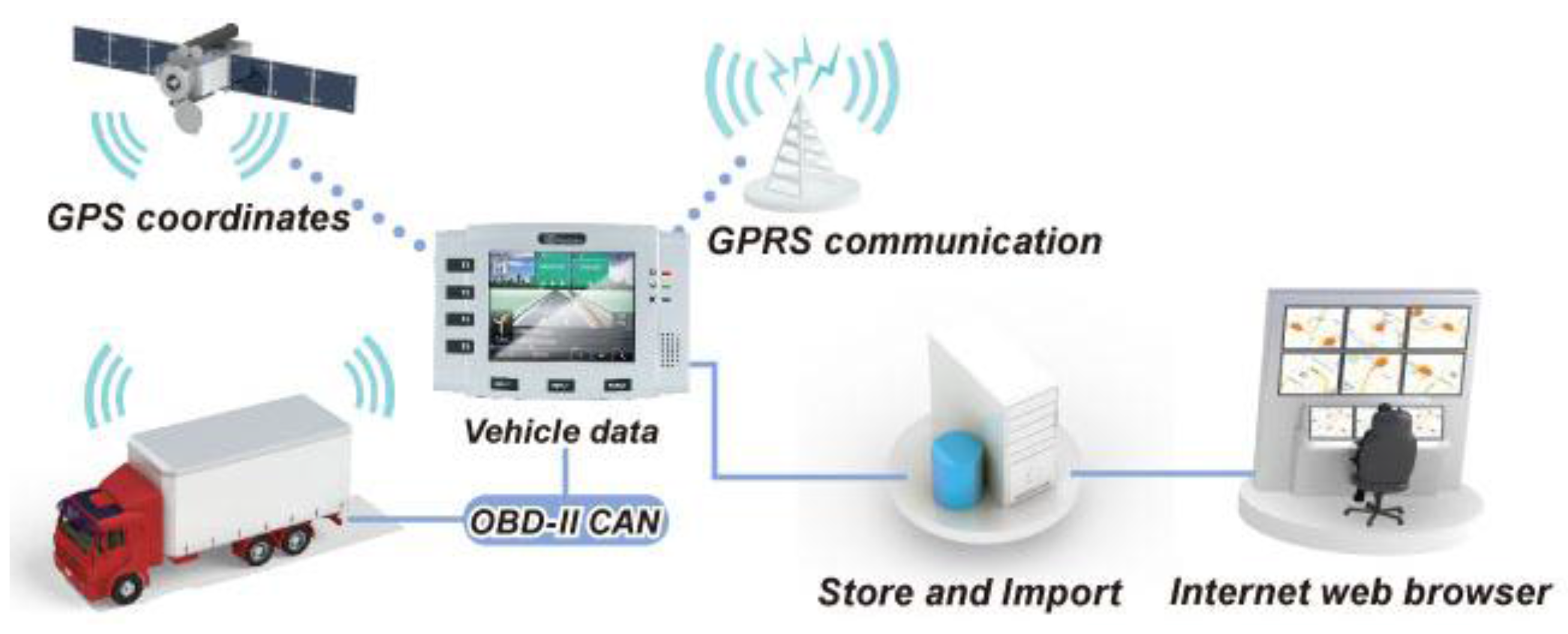
For a one working day, shift the tracking system installed in the truck provided approximately 760 GPS sampling points. In total, 152 trips were recorded, representing a total of 16,640 km travelled in total. Driving occupied on average 69.17% of the time per shift, an average 12.48% of the working shift corresponded to legal breaks, and refilling the truck’s fuel tank took 1.91%. Total loading and unloading times during the work shift constituted 9.55% and 6.88%, respectively. Per trip, the productivity of loading and unloading an average truck volume capacity of 69 m3 was 2.55 m3/min loading and 1.97 m3/min unloading.
During a working shift, Nurminen and Heinonen [
26] found that driving occupied was approximately 59%, while in Holzleitner
et al. [
8] found it was 60%, based on an average trip distance of 50 km. The average driving time was 9 h and the total breaks taken by the driver added to an average of 1.5 h (
Table 3). These values complied with the EU road transport working time directive. This working time directive states that a driver can drive for a maximum of 9 h in one day. This can be increased to 10 h twice a week resulting in a total of 56 h in one week but only a total of 90 h in any two-week period. In terms of legal breaks, after 4.5 h driving, a driver must take a break of 45 min. This break can be replaced by breaks of at least 15 min each, distributed over the driving period [
27].
Table 3.
Time of different work operations.
Table 3.
Time of different work operations.
| Work Operations | Time (min) | % Time Used | Std. Dev. |
|---|
| Per shift | Driving | 543 | 69.17 | 90 |
| Legal breaks | 98 | 12.48 | 13 |
| Refuelling | 15 | 1.91 | 08 |
| Loading | 75 | 9.55 | 26 |
| Unloading | 54 | 6.88 | 14 |
| Per trip | Loading | 35 | 9.78 | 05 |
| Unloading | 27 | 7.54 | 07 |
| Driving loaded | 152 | 42.46 | 17 |
| Driving unloaded | 144 | 40.22 | 18 |
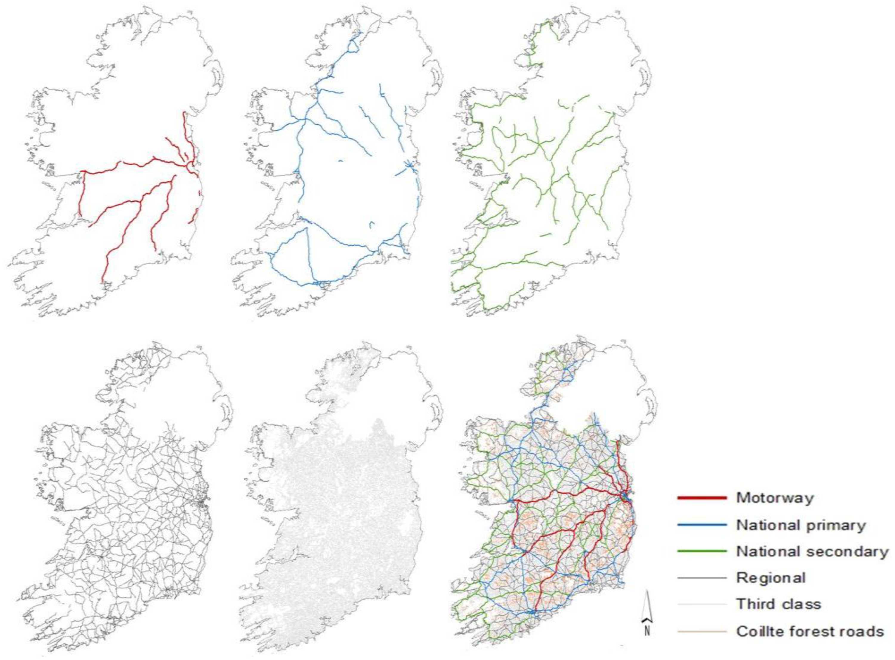
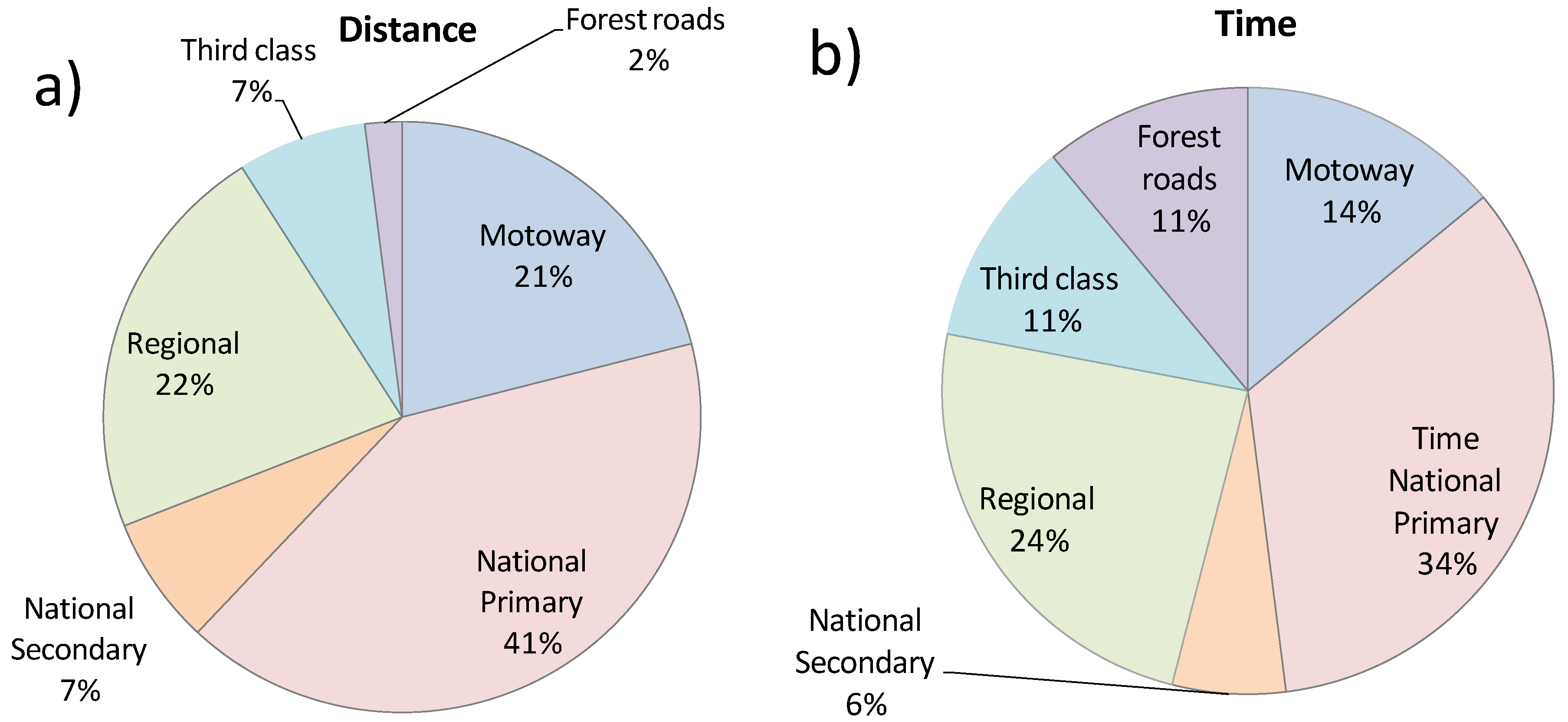
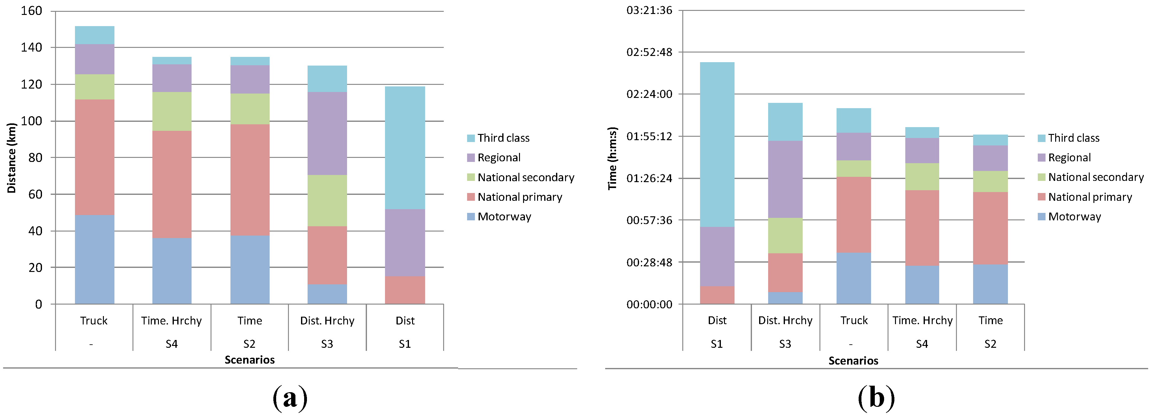
The travel distance per trip varied from 112 km to 197 km. The average loaded trip distance was 153 km, while for unloaded trips the average distance was 147 km—this represents 49% of back haulage. The road types in the road network were used in different proportions, with national primary and regional roads being the most used in terms of distance and time. The proportion of distance travelled on forest roads was an average of 2% or 4.38 km (
Figure 4). An Austrian study by Holzleitner
et al. [
8] presented an average distance travelled per trip on forest roads of 7.7 km. Transportation time is dependent on factors such as driver performance, truck engine, road and track conditions, weather,
etc. These factors were held constant throughout the analysis as in Dahal and Mehmood [
10].
Figure 4.
Average (a) distance and (b) time per road type.
Figure 4.
Average (a) distance and (b) time per road type.
3.3. Determination of Best Routes for Biomass Haulage
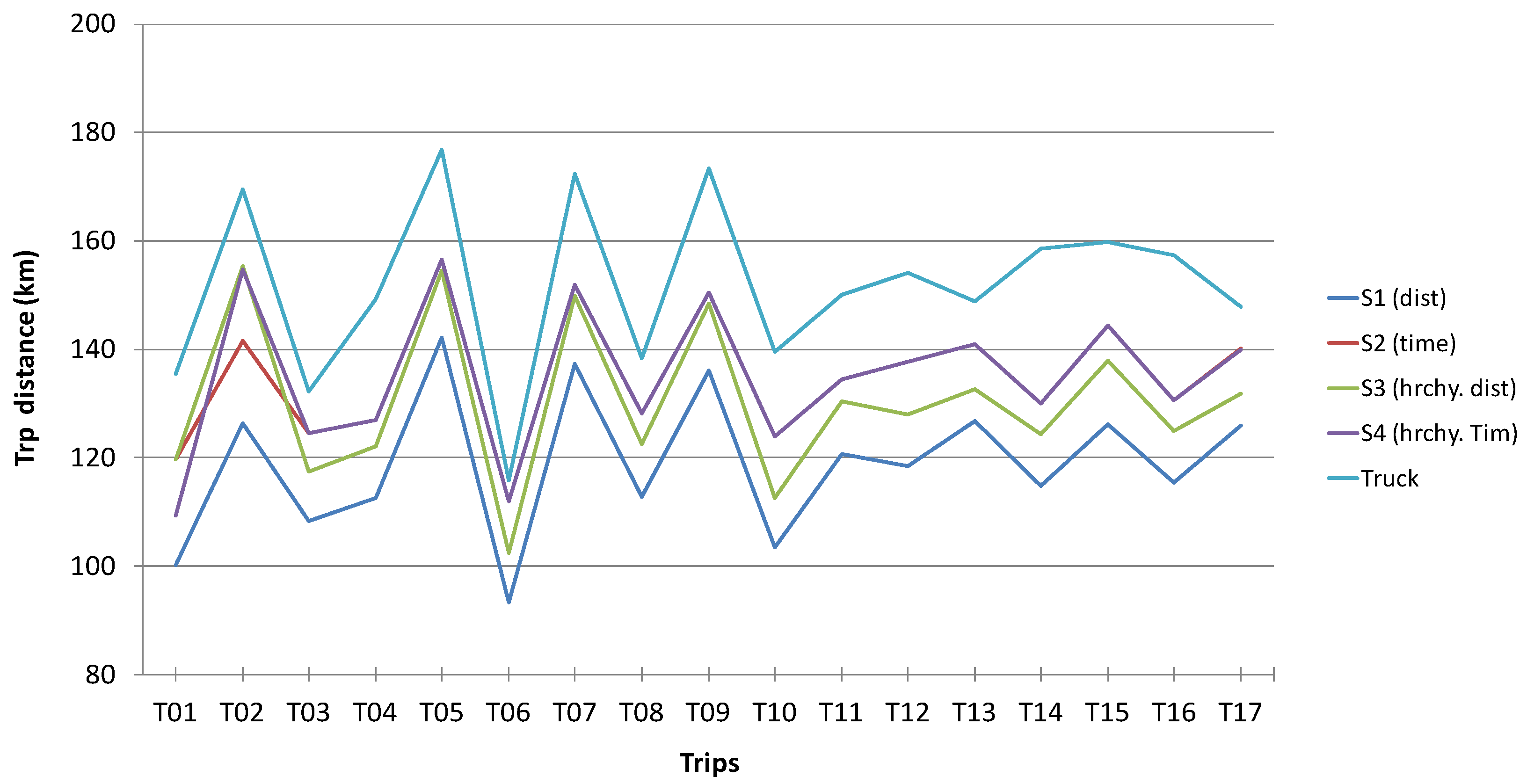
Trips taken by the truck from 17 different harvest areas to the mill were identified and analysed, a total of 68 routes resulted from the four scenarios evaluated with NA. The transport distances from all these routes are presented in
Figure 5. All the routes chosen by the truck driver were the longest in term of distance with an average 151.72 km, followed by scenarios S2 and S4 (134.91 km and 135.06 km, respectively). On the other hand, the minimum distance resulted from routes in S1, with average routes of 118.21 km, followed by S3 with average distance of 130.27 km (
Table 5).
Figure 5.
Comparison of travelling distance per trip under five different routing scenarios: shortest distance (S1), shortest time (S2), hierarchical shortest distance (S3), hierarchical shortest time (S4), and routes taken by the truck (S5).
Figure 5.
Comparison of travelling distance per trip under five different routing scenarios: shortest distance (S1), shortest time (S2), hierarchical shortest distance (S3), hierarchical shortest time (S4), and routes taken by the truck (S5).
The routes originated based on shortest distance had the longest travelling time (S1 and S3), with routes in S1 having an average driving time of 2 h and 46 min, approximately 19% more time than the routes taken by the truck. Routes in scenarios S2 and S4 had approximately 30% less driving time than S1. The driving time of the routes selected by the truck driver were in the middle in terms of time with an average of 2 h and 14 min per trip (
Table 5).
Table 5.
Summary of average distances and time per route under different scenarios.
Table 5.
Summary of average distances and time per route under different scenarios.
| Road class | (S1) Distance | (S2) Time | (S3) Distance (hierarchy) | (S4) Time (hierarchy) | Truck |
|---|
| Distance (km) | Motorway | 0 | 37.63 | 11.03 | 36.21 | 48.86 |
| National primary | 15.11 | 60.80 | 31.38 | 58.50 | 63.05 |
| National secondary | 0.2 | 16.65 | 28.07 | 21.35 | 13.54 |
| Regional | 36.44 | 15.56 | 45.33 | 14.97 | 16.57 |
| Third class | 67.11 | 4.29 | 14.46 | 4.04 | 9.70 |
| Total | 118.21 | 134.91 | 130.27 | 135.06 | 151.72 |
| Time (h:m:s) | Motorway | 0 | 00:27:12 | 00:08:12 | 00:26:31 | 00:35:19 |
| National primary | 00:12:13 | 00:49:58 | 00:26:33 | 00:48:44 | 00:51:49 |
| National secondary | 00:00:10 | 00:14:16 | 00:24:46 | 00:18:33 | 00:11:36 |
| Regional | 00:40:35 | 00:17:37 | 00:52:50 | 00:17:10 | 00:18:45 |
| Third class | 01:53:11 | 00:07:21 | 00:25:32 | 00:07:01 | 00:16:38 |
| Total | 02:46:10 | 01:56:24 | 02:17:54 | 01:57:59 | 02:14:08 |
Shortest path routes determined by S1 and S3 did not replicate the actual routes taken by the truck. Routes selected based on shortest driving time S2 and S4 agreed 99% on the driving directions, while the routes taken by the truck coincided 77% with the driving directions of routes from scenario S2 and S4. An example of the geographical representation of the routes under different scenarios can be seen in
Figure 6. The routes selected by the truck drivers demonstrate that the shortest distance routes are not necessarily the best routes for the truck drivers. Truck drivers have preferences on the types of roads they take; these preferences can be described by road features such as road length, quality, width, slope, speed limits,
etc. [
18].
Different proportions of road types were chosen in each scenario, when the objective was to find the shortest distances, routes presented a higher proportion of third class and regional roads (S1 and S3). When the objective was to find the routes based on shortest time (S2 and S4), the routes presented a higher proportion of national primary roads and motorways (
Figure 7).
Figure 6.
Geographical representation of routes under different scenarios and selected by the truck driver.
Figure 6.
Geographical representation of routes under different scenarios and selected by the truck driver.
Figure 7.
Different proportions of road types by routes under different scenarios: (a) by distance; (b) by time.
Figure 7.
Different proportions of road types by routes under different scenarios: (a) by distance; (b) by time.
The lower the kilometres travelled per litre of diesel, the higher the fuel consumption, resulting in increased cost per kilometre and thus decreased revenue per kilometre. Low km per litre also implies more kilograms of CO
2 emitted into the atmosphere. Fuel consumption by trucks is one of the largest contributors of greenhouse gases (GHGs) [
5]. Carbon dioxide emissions are directly related to the amount of diesel burned and one litre corresponds to 2.67 kg of CO
2 [
29]. Based on the average distances per trip presented in
Table 5 (
Section 3.3) and taken into consideration that the driver delivered two loads per workday, choosing the shortest distance routes (S1) implied a reduction in CO
2 emissions of 12% in comparison to S2 and S4.
Dockets from the weighbridge at the mill recorded the weight of the loads supplies during the study. The average truck payload was 28,300 kg (±1500 kg) and complied with the Irish vehicle regulations, as the truck weighed less than the legal maximum gross vehicle weight of 44,000 kg. Average fuel consumption per unit of production (ton) was 19.63 L/ton (±1.02 L).
The cost calculation of truck transportation was divided into those that are independent of the transportation distance and costs that depend on distance (
Table 6). With approximately 55,920 truckloads carrying the round wood harvested in 2013, and an average running cost of 0.83 €/km, choosing routes based on shortest distance instead of the ones chosen by the ones the truck used could translate into 1.5 million euro savings per year. However, these shortest distance routes are composed mostly of low class roads (third class), increasing road maintenance costs for Local Authorities and problems with public safety. Choosing routes with shortest distance but that prioritises higher road classes can produce approximately 0.8 million euro savings per year in comparison with the routes selected by the truck driver.
Table 6.
Truck and trailer standing and running costs for six axle articulated truck [
30].
Table 6.
Truck and trailer standing and running costs for six axle articulated truck [30].
| Description | Truck | Trailer |
|---|
| Cost basis | Vehicle cost (€) | 86,000 | 33,000 |
| Depreciation years | 6 | 10 |
| Average km annually | 120,000 | 40,000 |
| Working days annually | 240 | 240 |
| Average tyre life km | 100,000 | 50,000 |
| Standing costs per annum | Wages (€) | 38,000 | 0 |
| Depreciation (€) | 14,333 | 3300 |
| Road tax (€) | 2600 | 0 |
| Insurance (€) | 5300 | 400 |
| Interest (€) | 4300 | 1500 |
| Overhead per vehicle (€) | 14,497 | 0 |
| Standing cost per annum (€) | 79,337 | 5200 |
| Standing cost per day (€) | 330.6 | 22 |
| Running cost per km | Cost of 1 litre of fuel (net of vat) (€) | 0.97 | 0 |
| Litres per 100 km’s | 64 | 0 |
| Km’s per litre | 1.56 | 0 |
| Fuel cost per km (€) | 0.62 | 0 |
| Tyres (€) | 0.06 | 0.06 |
| Maintenance/Repairs (€) | 0.04 | 0.05 |
| Running cost per km (€) | 0.72 | 0.11 |
Transportation cost per ton was sensitive to the transportation distance. Fuel consumption per unit of production in general is affected by the hauling distance; the greater is the hauling distance, the higher is the fuel consumption per unit of production [
5]. Nurminen and Heinonen [
26] analysed different types of truck configurations and concluded that the use of semi-trailer trucks were more competitive due to a bigger load size, increasing productivity per hour and when transportation distances increased.
An important problem in forest operations is how to organise daily trips for a truck or fleet of trucks from different stands to different demand plants [
31]. The aim of truck scheduling is to maximise the utilisation of the truck’s capacity during a day. Therefore, when selecting the routes, travel time can be a much more crucial parameter to analyse rather than distance in terms of transportation costs. Choosing the routes generated in scenario S2 and S4 over S1 and S3 implied an increase in distance by 12%, but a decrease in time of 30%. This decrease in time allow trucks to be within the legal maximum driving time, while being able to deliver two loads, which it could not be possible following the routes in S1 and S3. Less driving time translates into better driving conditions across higher classes or roads, less wear and tear of trucks, less diesel and overall less expense for hauliers.


