Article

A Novel, Stable, and Economic Power Sharing Scheme for an Autonomous Microgrid in the Energy Internet

1
School of Electrical Engineering, Wuhan University, Wuhan 430072, China
2
Department of Electrical Engineering and Computer Science, the University of Tennessee, Knoxville, TN 37996, USA
*
Author to whom correspondence should be addressed.
Energies 2015, 8(11), 12741-12764; https://doi.org/10.3390/en81112338
Submission received: 16 September 2015 / Revised: 2 November 2015 / Accepted: 4 November 2015 / Published: 11 November 2015
(This article belongs to the Special Issue Decentralized Management of Energy Streams in Smart Grids)

Abstract

:
With a higher penetration of distributed generation in the power system, the application of microgrids is expected to increase dramatically in the future. This paper proposes a novel method to design optimal droop coefficients of dispatchable distributed energy resources for a microgrid in the Energy Internet considering the volatility of renewable energy generation, such as wind and photovoltaics. The uncertainties of renewable energy generation are modeled by a limited number of scenarios with high probabilities. In order to achieve stable and economical operation of a microgrid that is also suitable for plug-and-play distributed renewable energy and distributed energy storage devices, a multi-objective optimization model of droop coefficients compromising between operational cost and the integral of time-weighted absolute error criterion is developed. The optimization is solved by using a differential evolution algorithm. Case studies demonstrate that the economy and transient behavior of microgrids in the Energy Internet can both be improved significantly using the proposed method.

1. Introduction

Due to the environmental and geopolitical costs of fossil fuels, a federal program was created to stimulate essential innovation in energy technologies, such as wind and solar power [1,2,3,4]. In China, the cumulative installed capacity of wind power will reach 100 GW by 2015 and will easily meet the target of 200 GW by 2020 [5,6]. However, renewable energy sources have a fluctuating and unpredictable nature. Due to these characteristic uncertainties, the ever-increasing level of renewable energy sources in the power system makes system operation a challenging task and can introduce higher operational costs and stricter network constraints [7,8,9,10,11].
Recently, the concept of an “Energy Internet,” has been proposed by the Industrial Internet Consortium (IIC) and it is thought that microgrids in the Energy Internet can provide promising solutions [12]. The advantages of microgrids in the Energy Internet include supplying more reliable power to loads, integrating more renewable energy into power system, increasing energy utilization efficiency, and offering plug-and-play capabilities of distributed energy resources (DERs) and distributed energy storage devices.
To realize proportional power-sharing among distributed generations (DGs), some theoretical optimization methods and control schemes for Energy Internet microgrids have been proposed. Liu et al. [13] presented a model of multi-objective economic dispatch of the microgrid system, including Vehicle-to-Grid using the judgment matrix method for converting the multi-objective functions to a single objective function. In [14], Hawkes et al. developed a linear programming-based annual cost minimization model for unit commitment of generators and storage in a microgrid. A new distributed real-time electricity allocation scheme for the smart grid/microgrids energy management system (EMS) was proposed in [15]; its objectives are to reduce the electricity bills of residential customers, to increase the overall social benefit of the smart grid/microgrids community, and to increase the energy efficiency and reliability of the microgrids to rely on locally-generated electricity. Mohamed et al. [16] created a cost optimization scheme for a microgrid taking into account the costs of fuel, operation, maintenance, start-up, and emission. However, the implementation of the optimum economic solutions derived by [13,14,15,16] requires a centralized control system and additional communications infrastructure, which would result in a rise of investment cost and also limit the expansion of microgrids. The power sharing schemes addressed in these papers do not include any stability-related analysis and, thus, there is no guarantee the stability of microgrids could be maintained in the stated economic supporting operation conditions. In fact, the economic justifications may sometimes collide with the stability requirements.
Several control methods have been proposed to improve the stability of an autonomous microgrid. Nguyen et al. [17] proposed a new flywheel energy storage system based on a doubly-fed induction machine and a battery for use in microgrids that can control its power to compensate for fluctuations in wind power in grid-connected mode, in addition to controlling the frequency and voltage of the microgrid in islanded mode. Su et al. [3] proposed an adaptive robust total sliding-mode control system for the microgrid stability controller. It is proven that the adaptive, robust total sliding-mode control system is insensitive to parametric uncertainties and external disturbances. An improved dynamic model for the energy storage system in the context of grid-connected microgrids is proposed in [18]. Based on the model, a Proportional-Integral-Resonant DC link voltage controller is introduced to maintain the DC link voltage through the charging-discharging control of ultracapacitors and is capable of working properly under all operating conditions. However, these papers focus on advanced control methods to improve the stability of the microgrid and most of these rely on the centralized and communicated power-sharing schemes.
Compared to the centralized and communicated power sharing schemes mentioned above, a droop control is more desirable due to its reliability and robustness [19,20,21]. Under this circumstance, dispatchable distributed energy resources (DDERs) are controlled based on the droop characteristics to share the unbalanced power between outputs of non-dispatchable distributed energy resources (NDERs) and loads using local measured information. Inspired by the aforementioned consideration, this paper presents a multi-objective optimization model of droop coefficients compromising between the operational cost and the integral of time-weighted absolute error (ITAE) criterion. The detailed ITAE criterion is defined in [22] and has the advantage of producing smaller overshoots and oscillations. The model improves the dynamic behavior of the microgrid and is suitable for plug-and-play of distributed renewable energy and distributed energy storage devices. The proposed power sharing scheme can preserve not only the economic dispatch among DDERs, but also the stability of microgrids at all possible operating conditions. Due to the nonlinearity and complexity of the proposed optimization problem, the differential evolution (DE) algorithm is applied to solve the problem. The effectiveness of the proposed method has been demonstrated via numerical simulations on MATLAB R2013a/Simulink (The MathWorks, Natick, Massachusetts, MA, USA).
The original contribution of this paper is to provide an insight as to how to manage a decentralized droop control-based microgrid, from both an economic- and a stability-based viewpoint, via simply scheduling the droop coefficients. The remainder of this paper is organized as follows. In Section 2, description of the microgrid in the Energy Internet is presented. In Section 3, the multi-objective optimization model of droop coefficients considering the volatility of wind and solar power generation is proposed. Simulation results are provided to demonstrate the proposed method in Section 4. Conclusions are drawn in Section 5.

2. Microgrid in the Energy Internet Description

Figure 1 shows the structure of the microgrid in the Energy Internet used in this study. It is a cluster of distributed resource units and loads, serviced by a distribution system, and can operate in (1) grid-connected mode; (2) islanded (autonomous) mode; (3) ride-through between the two modes. Under normal circumstances, the microgrid shown in Figure 1 operates in autonomous mode. However, when it is subjected to large disturbances, such as loss of generating units or major lines, the system must operate in grid-connected mode. As a benefit of the droop control strategy, the plug-and-play of distributed renewable energy, distributed energy storage devices, and added loads can be easily realized. Therefore, there are two parts of the studied structure: the exited part and the extended part. In the exited part, three DDERs, a wind turbine generator (WTG), a photovoltaic plant (PV), an energy storage system (EES) and the commercial loads are installed at the main bus. For achieving a more refined load management, the commercial loads are divided into two groups: interrupted loads (IL) and non-interrupted loads (NL). The inverter controllers of WTG and PV employ the maximum power point tracking (MPPT) concept to output the captured wind and solar power to the system. All of the inverter controllers of DDERs employ the droop control concept to automatically undertake the unbalance power when the wind and solar power and the commercial loads change. The inverter controller of the EES employs V/f droop control to support the voltage and frequency of the system in the transient process through adjusting the output power by testing the change of terminal voltage and frequency. The extended part can include one or more DGs or other added commercial loads. The important note is that the microgrid must operate in grid-connected mode when a new unit has been interfaced into the system. Appendix A shows the detailed configuration of the microgrid.
Figure 1. Structure of a microgrid in the Energy Internet.
Energies 08 12338 g001

3. The Economic and Stable Power Sharing Scheme

3.1. Modeling of Wind and Solar Power Uncertainties

3.1.1. Wind Power Forecast

Wind is a fluctuating power source. Therefore, it is necessary to predict the power output of wind generators for the next few hours to days ahead as accurately as possible. As wind power cannot be predicted with 100% accuracy, it is possible that the actual wind power could be different from the forecasted one. In this paper, we assume that the wind power forecast is available and the wind power forecast error is simulated based on the Auto-Regressive and Moving Average Model (1, 1) (ARMA) model, which was originally proposed in Wind Power Integration in Liberalised Electricity Markets (WILMAR) project [20,21,22,23,24].
It is assumed in the ARMA (1, 1) model that the wind power forecast error is subject to a normal distribution N ( 0 , σ t 2 ) in each time interval t. The variance series of wind power forecast error can be calculated as:
V 0 = 0 V 1 = σ z 2 V t = μ 2 V t 1 + ( 1 + ν 2 + 2 μ ν ) σ z 2
Correspondingly, the standard deviation series σ t is calculated as:
σ t = V t
The parameters σ Z , μ, and ν in ARMA (1, 1) model can be identified by fitting the forecast error series as close as possible to available historical data.
In Figure 2, the time series of the forecasted wind power with its 95.4% probability interval ( ± 2 σ t ) are shown.
Figure 2. Forecasted wind power and its 95.4% probability interval.
Energies 08 12338 g002

3.1.2. Scenario Generation

The wind power scenarios representing the future realization of uncertainties are generated using the Latin hypercube sampling (LHS) technique in this paper. LHS is a stratified sampling method which is very efficient at extracting samples from the entire distribution of random variables [25]. Compared to the traditional Monte Carlo Simulation which randomly samples the cumulative distributions to obtain variable inputs, LHS uniformly samples the cumulative distributions and approximates the required normal distribution much better [26]. The procedure for LHS can be divided into two main steps; sampling and permutation. The objective of sampling is to generate representative samples to cover probabilistic distributions of each input random variable (wind power at different time stage). The permutation aims at reducing the correlations between samples of different input random variables using the Cholesky decomposition method [27].
In our experiment, a scenario set with 3000 scenarios is generated. To alleviate the computational burden this scenario set must be reduced to contain only a finite number of scenarios which represent the original process as closely as possible.

3.1.3. Scenario Reduction

A scenario reduction technology is employed to determine a set with the requested number of scenarios and assign optimal probability to the preserved scenarios. The scenarios with very low probability will be eliminated and the close scenarios will be aggregated by measuring the distance of probability distribution between every pair of scenarios [28]. The initial scenario set with 3000 scenarios is ultimately reduced to 10 scenarios, as shown in Figure 3.
The modeling of solar power uncertainties is congruent to wind power and will not be repeated here. A scenario tree for stochastic solar power is shown in Figure 4 and the numerical results of scenario generation and reduction are shown in Appendix B.
Figure 3. Scenario tree for stochastic wind power.
Energies 08 12338 g003
Figure 4. Scenario tree for stochastic solar power.
Energies 08 12338 g004

3.2. Dynamic Power Sharing Scheme

The assignment of a droop coefficient to each DDER in the traditional method is usually based on an equitable load share in the form of mp1P1 = mp2P2 = … =mpnPn = constant, nq1Q1 = nq2Q2 = … = nqnQn = constant, where Pi and Qi are the rated active and reactive power output of DDER i [19]. It is remarkable that neither the economic nor the stability content is considered therein; the droop coefficients of the DDERs are scheduled based on rated power only. In fact, the operational cost and the stability of the microgrid are all closely related to the assignation of droop coefficients.
In this paper, a droop-based power sharing scheme uses the frequency and voltage of the microgrid as a common signal among the DDERs to balance the active and reactive power mismatch between generation and demand. The power injected from DDER i is mainly determined by its droop coefficient mpi and nqi, which has been proposed in the preliminary work published in [29]. It is shown in Appendix C.

3.3. Multi-Objective Optimization Model of Droop Coefficients

3.3.1. Pareto-Optimality Concept and Multi-Objective Optimization

A multi-objective optimization problem can be described using the following formulation:
min y = F ( x ) = { f 1 ( x ) , f 2 ( x ) , ... , f n ( x ) } x R m , y R n
while fp(·) is the pth objective function (for 1 ≤ pn).
In most cases, there does not exist a global optimal solution to such a problem. However, the Pareto-optimality concept has been intensively used and solutions included in the Pareto-optimal set are those that cannot be improved along any dimension without simultaneously deteriorating along another dimension(s) [30].

3.3.2. Mathematical Formulation of the Proposed Problem

To minimize the total operational cost, the droop coefficient of each DDER should be selected carefully so that the DDERs with high and low fuel cost can be forced to share a relatively small and large portion of unbalanced power between generation and demand. On the other hand, the stability of a microgrid is also largely affected by the selection of droop coefficients. With inappropriate settings, a large overshoot or oscillation would appear in the transient process of the microgrid with the variation of renewable energy generation and load. In order to achieve both the economic dispatch among multiple DDERs in steady state and the satisfactory dynamic behavior of the microgrid in transient with the variation of operating conditions, a multi-objective optimization model of droop coefficients compromising between the operational cost and the ITAE criterion is proposed, which indicates the dynamic behavior of the microgrid. The multi-objective function is defined as:
min C = ω 1 × f 1 + ω 2 × S C × f 2
where f1 is the operational cost and f2 is the ITAE criterion. SC is the scaling factor, blending f2 with f1, and ω1 and ω2 are the weighting factor whose value varies between [0, 1].
The operational cost f1 is formulated as:
f 1 = [ t = 1 N t i = 1 N i F C i t ( P i , n e w t ) + t = 1 N t i = 1 N i k = 1 N k α k E F i , k P i , n e w t + C n e t × E n e t ] t N t , i N i , k N k
where P i , n e w t is the steady state power output of DDER i at time stage t; F C i t ( P i , n e w t ) is the fuel cost of DDER i at time stage t; αk is the externality cost of emission type k (such as nitrogen oxides (NOx), sulfur oxides (SO2), carbon oxides (CO2), and so on); EFi,k is the emission factor of DDER i, emission type k; Nt, Ni, and Nk are the numbers of time stages, DDERs, and emission types, respectively; Enet is the planned exchange electric quantity between the microgrid and the main grid during the scheduling period and indicates that the microgrid purchases electricity from the main grid when the value is positive, and vice versa; and Cnet is the purchase or sale of electricity price for microgrid, which can be descripted as piecewise function:
C n e t = { C b , E n e t > 0 C s , E n e t < 0
where Cb and Cs are the purchase or sale of electricity price for the microgrid, respectively.
The planned exchange electric quantity between the microgrid and the main grid during the scheduling period T can be calculated by Equation (7):
E n e t = 0 T P n e t d t
where Pnet is the constant exchange power between the microgrid and the main grid during the scheduling period T, which indicates that the power flows from main grid to the microgrid when the value is positive, and vice versa.
It can be seen in Equation (5) that f1 is composed of fuel costs and environmental externality costs over the scheduled horizon. The operational costs of WTG and PV are assumed to be zero.
The fuel cost of DDER i at time stage t is modeled as a quadratic function of steady state power output of DDER i, as:
F C i t ( P i , n e w t ) = a F i + b F i P i , n e w t + c F i ( P i , n e w t ) 2 t N t
where aFi, bFi, and cFi are the cost coefficients of DDER i.
The ITAE criterion f2 is formulated as:
f 2 = k = k 0 T 0 ( k k 0 ) W E a b s ( k )
where k is the current sample time; k0 is the starting time of wind generation and load change; T0 is ending time of calculation; W is the weighting matrix which is an identity matrix in this paper; and Eabs(k) is the absolute error vector and it is defined as:
E a b s ( k ) = [ t = 1 N t | f n e w t f t ( k ) | , t = 1 N t j = 1 N j | V j , n e w t V j t ( k ) | , t = 1 N t i = 1 N i | P i , n e w t P i t ( k ) | , t = 1 N t i = 1 N i | Q i , n e w t Q i t ( k ) | ] T t N t
where f n e w t is the steady state frequency of the microgrid at time stage t; V j , n e w t is the magnitude of steady state voltage of bus j; Nj is the number of buses; Q i , n e w t is the steady state reactive power output of DDER i at time stage t; and f t ( k ) , V j t ( k ) , P i t ( k ) and Q i t ( k ) are the measured frequency, voltage magnitude of bus j, power, and reactive output of DDER i at time stage t, respectively.
The objective function Equation (4) is subject to a set of operational constraints including the frequency and voltage regulation constraints and DDER capacity constraints. All these constraints are summarized as:
f min f t ( k ) f max V j min V j t ( k ) V j max ( P i t ( k ) ) 2 + ( Q i t ( k ) ) 2 S i max
where fmin and fmax are the allowed minimum and maximum frequency, V j min and V j max are the lower and upper limits of bus j voltage magnitude, and S i max is the inverter capacity of DDER i.
The objective function Equation (4) is subjected to a set of system constraints, including the power balance constraints, generating constraints, EES constraints, operational reserve constraints, frequency, and voltage regulation constraints and scenario constraints. All the constraints are summarized as follows.
(1) Power balance constraints
i = 1 N i P i t + P W t + P P t + P E t + P n e t = P N L t + P I L t t N t , i N i
where P W t and P P t are the forecasted wind and solar power generation at time t; P E t is the exchange power of EES at time t; P N L t and P I L t are the non-interrupted and interrupted loads at time t. Notice that the network loss is not considered here.
(2) Generation constraints
P i , min P i t P i , max i N i , t N t
where P i , min and P i , max are the lower and upper operating limits on generation of DDER i, respectively.
(3) EES constraints
The charge or discharge electric quantity of EES during period T is as:
E E t = 0 T P E t d t t N t
The residual electric quantity of EES at the end of period T is as:
E r t = E i n t + t = 1 T E E ( T ) t N t
where E i n t is the initial electric quantity of EES.
The electric quantity and power constraints of EES are as:
E E , min E r t E E , max t N t
P E , m i n P E S S t P E , max t N t
where E E , min , E E , max , P E , m i n and P E , max are the lower and upper operating limits of the electric quantity and exchange power of EES, respectively.
(4) Operational reserve constraints:
In order to ensure the non-interrupted loads maintain continuous operation, all the power output of the microsources must be greater than the power demand of non-interrupted loads, considering the microgrid is likely to disconnect from the main grid at any time.
i = 1 N i P i , max + P E , max + P W t + P P t P N L ( k ) t N t , i N i
Meanwhile, in order to ensure the non-interrupted loads keep continuous operation for a period T at the end of time t, the whole electric quantity of the microgrid must be greater than the electric quantity demand of non-interrupted loads, as the energy storage constraints of EES.
E r t + i = 1 N i 0 T P i , m a x d t + 0 T P P t d t + 0 T P W t d t 0 T P N L t d t t N t , i N i
(5) Frequency and voltage regulation constraints
f min f t f max t N t
V min V t V max t N t
where f min , f max , V min and V max are the allowed minimum and maximum frequency and voltage, respectively, which are chosen as 49 Hz, 51 Hz, 0.95 p.u. and 1.05 p.u., respectively.
(6) Scenario constraints
For the sake of considering uncertainties of wind and solar power generation, the scenario constraints have been added to the model for the system power balance.
{ i = 1 N i P i t , s + P W t , s + P P t , s + P E t , s + P n e t = P N L t + P I L t P i , min P i t , s P i , max E E , min E r t , s E E , max P E , m i n P E S S t , s P E , max i = 1 N i P i , max + P E , max + P W t , s + P P t , s P N L ( k ) E r t , s + i = 1 N i 0 T P i , max d t + 0 T P P t , s d t + 0 T P W t , s d t 0 T P N L t , s d t f min f t , s f max V min V t , s V max t N t , i N i , s N s

3.3.3. Fuzzy Logic Theory Involving to the Differential Evolution (DE) Algorithm

The proposed optimization problem shown above is a constrained nonlinear optimization problem. DE is used because of its characteristic of being derivative-free and, thus, effective in capturing the optimal results. It is to be mentioned that in the optimization process, after calculating the objective function, all the constraints are checked and a penalty term is added if any constraint is violated. The algorithm stops if there is no improvement in the objective function.
The values of objective functions can usually belong to different intervals with variable lengths and some objective functions may be always dominated by the others. For example, if f i [ 10 2 , 10 3 ] and f j [ 0 , 1 ] ( i j , 1 i , j n ) , it is easy to find that the objective function f i is in a dominant position. In order to make the evaluation more efficient, fuzzy logic theory is used in the normalization of each objective function based on the following steps:
(1) Divide the interval of ω1 and ω2 into 10 subintervals and implement the optimization repeat from 0 to 1 with a step increment of 0.1. Two groups of non-dominated objective function f1,i and f2,i can be obtained and are presented in Table 1.
Table 1. Divisions of w and the objective function.
VariablesScenarios
i1234567891011
ω100.10.20.30.40.50.60.70.80.91
ω210.90.80.70.60.50.40.30.20.10
f1,if1,1f1,2f1,3f1,4f1,5f1,6f1,7f1,8f1,9f1,10f1,11
f2,if2,1f2,2f2,3f2,4f2,5f2,6f2,7f2,8f2,9f2,10f2,11
(2) Calculate the lower-bounds f1,min, f2,min and upper-bounds f1,max, f2,max of each objective function based on [30].
(3) For the two groups of non-dominated objective function f1,i and f2,i, a fuzzy membership function can be assigned as:
μ ( f 1 , i ) = { 1 , f 1 , i f 1 , min f 1 , max f 1 , i f 1 , max f 1 , min , f 1 , min f 1 , i f 1 , max 0 , f 1 , i f 1 , max μ ( f 2 , i ) = { 1 , f 2 , i f 2 , min f 2 , max f 2 , i f 2 , max f 2 , min , f 2 , min f 2 , i f 2 , max 0 , f 2 , i f 2 , max
(4) By choosing an appropriate ω, we can now reduce the multi-objective optimization to the minimization of the following fitness function:
F i t n e s s i = ω 1 μ ( f 1 , i ) + ω 2 μ ( f 2 , i )
(5) The best compromise solution can be found when the normalized sum of the membership function Equation (23) is highest:
C i = F i t n e s s i i = 1 11 ( F i t n e s s i )

4. Experimental Verification of Proposed Method

The exited part of the microgrid system depicted in Figure 1 is used to demonstrate the proposed approach for finding the optimal droop coefficients. The rated frequency and voltage of the microgrid is 50 Hz and 380 V, respectively. The inverter capacity of each DDER is 300 kVA. The passive filter of each microsource is rf = 0.1 Ω, Lf = 1.35 mH, Cf = 50 μF; the coupling resistance and inductance of each microsource is rc = 0.01 Ω, Lc = 0.02 mH. The fuel cost coefficients, output power limits and externality cost coefficients of three DDERs are listed in Table 2 and Table 3. The capacity and other coefficients of the EES are listed in Table 4.
The total load demand of the microgrid is shown in Table 5, with 50% non-interruptible load.
This paper solves the optimization model presented in Equations (1)–(21) using DE and determines the best compromise solution according to the fuzzy logic theory. The value of the objective function Equation (2) is 0.0375 and the corresponding optimal droop coefficients of DDERs are shown in Table 6. The convergence characteristic of the objective function using the DE algorithm is shown in Figure 5. It can be seen that the convergence of the objective function is fast and the DE algorithm is capable of finding the optimum of the proposed nonlinear optimization problem.
Table 2. Fuel cost coefficients of dispatchable distributed energy resources (DDERs).
Fuel Cost CoefficientsDDER 1DDER 2DDER 3
aFi ($)1.1505.71710.193
bFi ($/kWh)57.783100.937105.180
cFi ($/kW2h)−133.0915062.560
Pi,min(kW)101520
Pi,max(kW)200300400
Table 3. Externality costs and emission factors for NOx, SO2 and CO2.
Emission Type kαk ($/lb)EF1,k (lb/kWh)EF2,k (lb/kWh)
NOx4.2000.4400.400
SO20.9900.0080.006
CO20.0141.5961.378
Table 4. The coefficients of energy storage system (EES).
P E S S m a x (kW) E i n i (kWh) E E S S m a x (kWh) E E S S m i n (kWh)
1001020010
Table 5. Total load demand.
Time StageTotal Active Load (kW)Total Reactive Load (kVar)Time StageTotal Active Load (kW)Total Reactive Load (kVar)
1535175.813789259.3
2575189.014783257.4
3574188.615790259.7
4579190.316696228.8
5585192.317630207.1
6598196.618599196.9
7667219.219621204.1
8707232.420577189.7
9689226.521591194.3
10683224.522687225.8
11796261.623688226.1
12794261.024606199.2
Table 6. The optimal droop coefficients.
mp1 (rad/(s·W))mp2 (rad/(s·W))mp3 (rad/(s·W))nq1 (V/Var)nq2 (V/Var)nq3 (V/Var)
2.596 × 10−63.845 × 10−64.811 × 10−68.152 × 10−75.493 × 10−69.885 × 106
Figure 5. Convergence curve of objective function.
Energies 08 12338 g005
As shown in Table 7, under the control of these optimal droop coefficients, the system operation cost f1 is $1483.3 and the ITAE criterion f2 is 0.0229, respectively. If considering only the minimization of operational cost, which is ω1 = 1 and is utilized in Equation (2), f1 will be $1276.60, which is lower than $1483.3. However, f2 will be 0.3452, which is much larger than 0.0229. The system will have a poor dynamic response characteristic. On the other hand, if only considering the minimization of ITAE criterion, which is ω1 = 0 and is utilized in Equation (2), f2 will be 0.0124, which is lower than 0.0229. Here f1 will be $1846.10, which is much larger than $1483.3. The system will operate in an uneconomical power-sharing scheme. The above comparison further validates the necessity to take into account both economic and stability considerations in the design process of optimal droop coefficients.
Table 7. The optimal results of the power sharing scheme.
Weighing Factor ω1Weighing Factor ω2Operation Cost f1 ($)ITAE Criterion f2 ($)
0.50.51483.30.0229
101276.60.3452
011846.10.0124
To further demonstrate that the dynamic power sharing scheme will enhance the transient and dynamic stability of the system, a comparison of numerical simulations between operation curves is presented below. Figure 6, Figure 7, Figure 8 and Figure 9 shows the responses of system frequency, voltage amplitude of the main bus, active power of DDER2, and reactive power of DDER1 with the optimal droop coefficients (ω1 = 0.5, ω2 = 0.5) and the economy-based optimal droop coefficients (ω1 = 1, ω2 = 0). As shown in Table A1, scenario 6 has the largest occurrence probability for wind power and is used as an example. To mimic the variation of operating conditions in a day, the wind generation and load change every 10 s according to Table 5, Table A1 and Table A2.
Figure 6. (a) The system frequency response with the optimal droop coefficients (ω1 = 0.5, ω2 = 0.5); (b) The system frequency response with the economy-based optimal droop coefficients (ω1 = 1, ω2 = 0).
Energies 08 12338 g006
Figure 7. (a) The voltage amplitude response of bus3 with the optimal droop coefficients (ω1 = 0.5, ω2 = 0.5); (b) The voltage amplitude response of bus3 with the economy-based optimal droop coefficients (ω1 = 1, ω2 = 0).
Energies 08 12338 g007
Figure 8. (a) The response of DDER2 output active power with the optimal droop coefficients (ω1 = 0.5, ω2 = 0.5); (b) The response of DDER2 output active power with the economy-based optimal droop coefficients (ω1 = 1, ω2 = 0).
Energies 08 12338 g008
Figure 9. (a) The response of DDER1 output reactive power with the optimal droop coefficients (ω1 = 0.5, ω2 = 0.5); (b) The response of DDER1 output reactive power with the economy-based optimal droop coefficients (ω1 = 1, ω2 = 0).
Energies 08 12338 g009
It can be observed in group (a) of Figure 6, Figure 7, Figure 8 and Figure 9 that the microgrid has excellent dynamic performance with the optimal droop coefficients. When the wind generation and load change, the transient process exhibits a small overshoot, little regulation time, and rapid oscillation decay. All the operational constraints are maintained in the allowable range (the maximum frequency deviation is −0.16 Hz, the maximum voltage amplitude deviation is +0.5 V, and the maximum apparent power of DDERs is 241.1 kVA).
If only considering the minimization of operation cost, which is ω1 = 1, ω2 = 0, and is utilized in Equation (4), the system would probably have very poor dynamic performance with the variation of operating conditions. The system response with the economy-based optimal droop coefficients is shown in group (b) of Figure 6, Figure 7, Figure 8 and Figure 9. It can be observed that the transient process exhibits very large oscillations and the system will lose stability at time stage 19, 20 and 21.

5. Conclusions

This paper proposes a method for scheduling droop coefficients to simultaneously improve the economy and stability of a microgrid, considering the volatility of wind power generation. A multi-objective optimization model of droop coefficients compromising between the operational cost and the ITAE criterion is presented. The simulation result validates the effectiveness of the proposed method. It is emphasized in this paper that both the economy and the stability of microgrids should be taken into consideration in the design process of droop coefficients. If not, the autonomous microgrid may suffer economic hardship or stability degradation with the variation of wind generation or load demand.

Acknowledgments

The authors are grateful for the projects (51207113 and 51477121), supported by the National Natural Science Foundation of China.

Author Contributions

Bingke Yan and Bo Wang designed the main parts of the study, including microgrid modelling, droop control scheme design, optimization model formulating, and the implementation of algorithms, simulation, and experiments. Lin Zhu and Hesen Liu mainly contributed to the writing the paper. Yilu Liu was responsible for guidance, a number of key suggestions, and manuscript editing. Xingpei Ji and Dichen Liu were also responsible for some constructive suggestions.

Conflicts of Interest

The authors declare no conflict of interest.

Appendix

A. The Detailed Configuration of the Microgrid

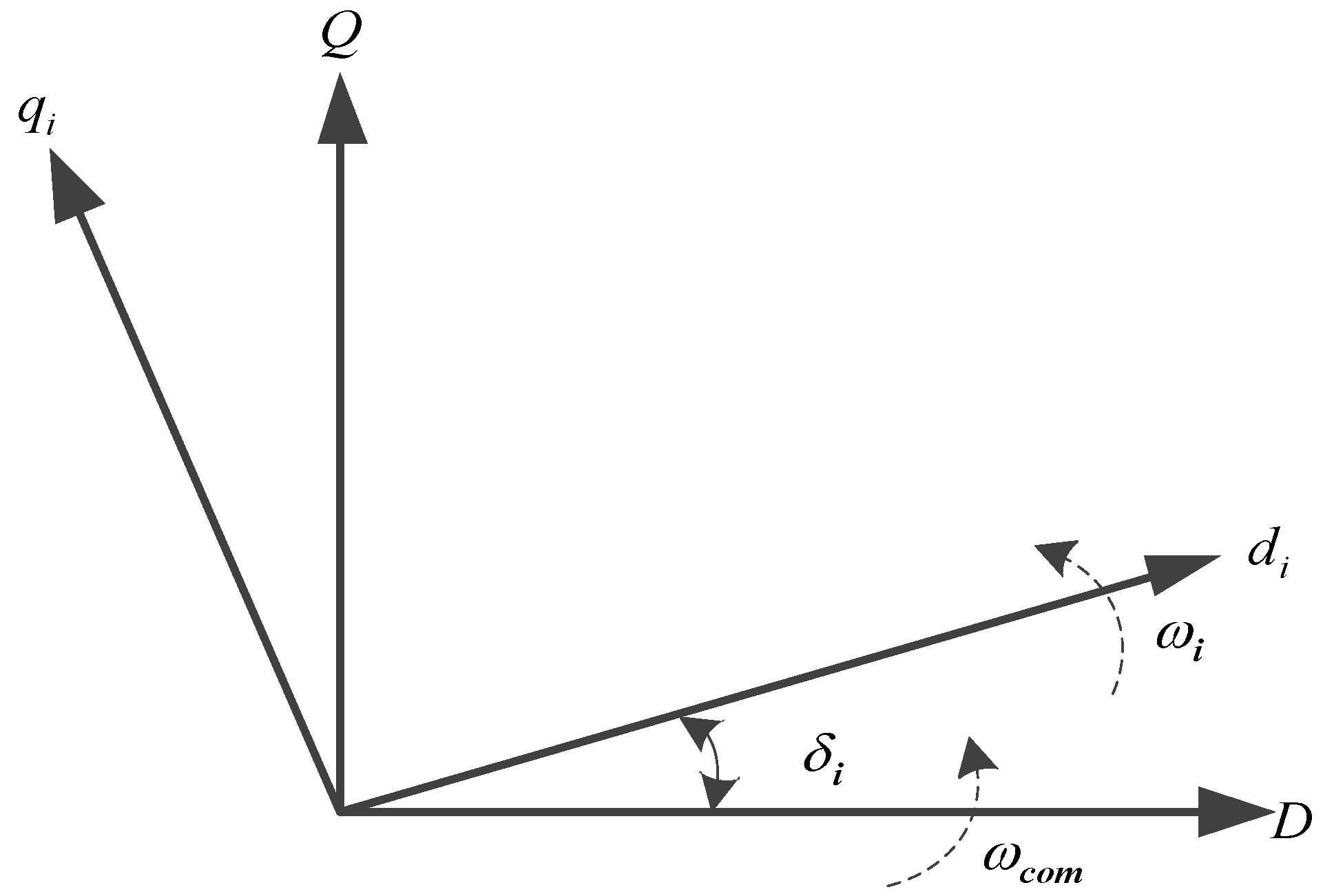
The model of each inverter is built on the individual reference frame di-qi rotating synchronously with the inverter output voltage angular speed ωi. To build the whole model of the system, the reference frame of one of the DDER interfaced inverters is chosen as the common reference frame D-Q rotating at the frequency ωcom, and all the other inverters are translated to this common reference frame using angle δi, which is defined as the angle between an individual reference frame and the common reference frame, as shown in Figure A1. δi is given as:
δ i = ( ω i ω c o m ) d t = θ i θ c o m
where θi and θcom are the rotating angle of individual reference frame and common reference frame, respectively.
Noted that in the following sections the three phase voltages and currents of each inverter model are represented as vectors in its individual di-qi frame and the network and loads are represented as vectors in the common D-Q frame.
Figure A1. Reference frame transformation.
Energies 08 12338 g010
(1) DDER Interfaced Inverter
Figure A2 shows the power circuit and control block diagram of the DDER interfaced inverter. The inverter model includes power controller, voltage and current controller, LC filter and coupling inductor.
Figure A2. Power circuit and control block diagram of DDER interfaced inverter.
Energies 08 12338 g011
(a) Power Controller
The power controller is used to generate the frequency and magnitude of the fundamental output voltage according to the droop characteristics set for the real and reactive powers. The block diagram of power controller is shown in Figure A3.
Figure A3. Block diagram of power controller.
Energies 08 12338 g012
First, the instantaneous active and reactive power components p and q are calculated from the measured output voltage and current as:
p = v o d i o d + v o q i o q q = v o d i o q v o q i o d
Second, the average active and reactive powers corresponding to the fundamental components are subjected to control actions, and they are obtained by means of a low-pass filter as:
P = ω c s + ω c p Q = ω c s + ω c q
where ωc represents the cut-off frequency of the filter.
Finally, the fundamental voltage frequency ω and d-axis voltage magnitude reference v o d are set according to the droop characteristics and q-axis voltage magnitude reference v o q is set to zero, as:
ω = ω n m p ( P P n ) d δ d t = ω ω c o m v o d = V n n q ( Q Q n ) v o q = 0
where ω n , V n , P n and Q n are the nominal frequency, voltage, active and reactive powers, respectively, m p and n q are the droop coefficients.
(b) Voltage Controller
The voltage controller is used to synthesize the reference filter-inductor current vector by employing standard proportional-integral (PI) regulators with feedback and forward terms. Figure A4 shows the block diagram of voltage controller. The corresponding state equations are given as:
d ϕ d d t = v o d v o d d ϕ q d t = v o q v o q
Along with the algebraic equations:
i l d = F i o d ω n C f v o q + K p v ( v o d v o d ) + K i v ϕ d i l q = F i o q + ω n C f v o d + K p v ( v o q v o q ) + K i v ϕ q
where K p v , K i v are the proportional and integral gains, respectively, and F is the feed forward gain.
Figure A4. Block diagram of voltage controller.
Energies 08 12338 g013
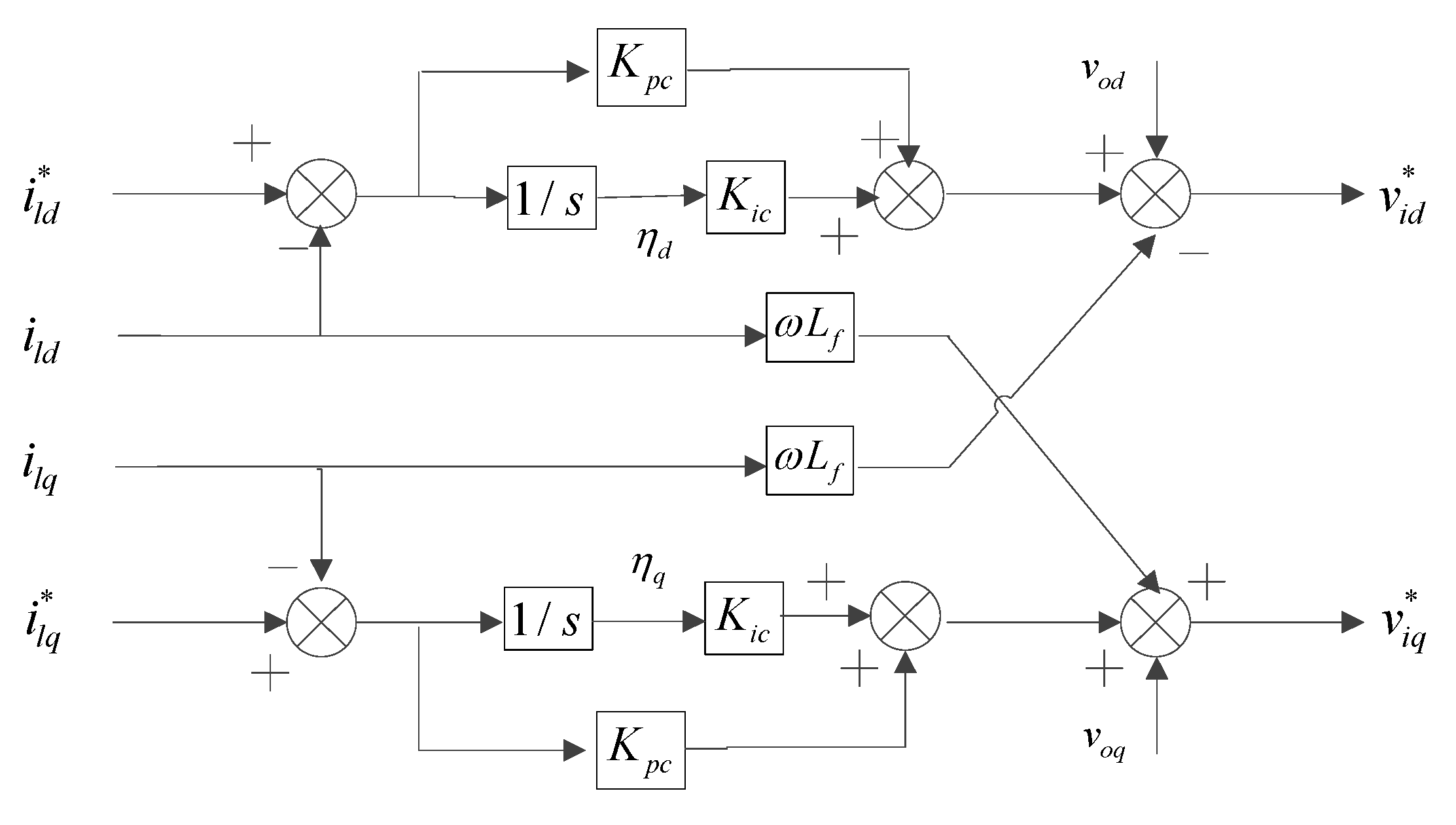
(c) Current Controller
The current controller is used to generate the command voltage vector which will be synthesized by a pulse-width-modulation (PWM) module of inverter. The structure of the PI current controller with feedback and forward control loops is shown in Figure A5. The corresponding state equations are given as:
d γ d d t = i l d i l d d γ q d t = i l q i l q
Along with the algebraic equations:
v i d = ω n L f i l q + K p c ( i l d i l d ) + K i c γ d v i q = ω n L f i l d + K p c ( i l q i l q ) + K i c γ q
where K p c , K i c are the current controller parameters.
Both the voltage and current controllers are designed to reject high frequency disturbance and damp the output of the LC filter to avoid any resonance with the external network.
Figure A5. Block diagram of current controller.
Energies 08 12338 g014
(d) LC Filter and Coupling Inductance
The LC filter and coupling inductance dynamics can be represented by the following equations, assuming that the inverter produces the demand voltage v i = v i .
d i l d d t = r f L f i l d + ω i l q + 1 L f v i d 1 L f v o d d i l q d t = r f L f i l q ω i l d + 1 L f v i q 1 L f v o q d v o d d t = ω v o q + 1 C f i l d 1 C f i o d d v o q d t = ω v o d + 1 C f i l q 1 C f i o q d i o d d t = r c L c i o d + ω i o q + 1 L c v o d 1 L c v b d d i o q d t = r c L c i o q ω i o d + 1 L c v o q 1 L c v b q
where r f , L f and C f are the resistance, inductance, and capacitance of the LC filter, r c and L c are the coupling resistance and inductance.
(2) WTG Interfaced Inverter
Figure A6 shows the power circuit and control block diagram of the wind turbine generator interfaced inverter. The inverter model includes phase-locked loop (PLL), DC bus capacitor, reactive power calculation, DC bus voltage and reactive power controller, current controller, LC filter and coupling inductor.
(a) PLL
The PLL form, shown in Figure A7, is adopted to provide the rotation frequency ω and reference angle θ for the rotating frame of inverter output voltage. θ is used to transfer the voltage and currents from abc to dq and vice versa. The PLL model can be written as:
d φ p l l d t = v o q d δ d t = ω ω c o m ω = K i p l l φ p l l + K p p l l v o q
Figure A6. Power circuit and control block diagram of wind turbine generator interfaced inverter.
Energies 08 12338 g015
Figure A7. Block diagram of PLL.
Energies 08 12338 g016
(b) DC Bus Capacitor
The DC power p w i n d coming from the rectifier will be instantaneously transferred to the inverter DC terminal through a capacitor, and then to the grid through inverter. Assuming the inverter is lossless, the voltage of DC bus capacitor can be expressed as:
C u D C d u D C d t = p w i n d ( v i d i l d + v i q i l q )
where C is the DC bus capacitance.
(c) Reactive Power Calculation
The average reactive power Q can be calculated as:
Q = ω c s + ω c ( v o d i o q v o q i o d )
(d) DC Bus Voltage and Reactive Power Controller
The DC bus voltage and reactive power controllers are used to set the d- and q-axis current reference to the inner current control loops, respectively. Figure A8 shows the block diagram of this controller. The corresponding state equations are given as:
d ε d d t = u D C u D C d ε q d t = Q * Q
Along with the algebraic equations:
i l d = K p D C ( u D C u D C ) + K i D C ε d i l q = K p Q ( Q * Q ) + K i Q ε q
where K p D C , K i D C , K p Q and K i Q are the proportional and integral gains of DC bus voltage and reactive power controller, u D C and Q * are the references of DC bus voltage and output reactive power of inverter ( Q * is usually set to zero).
Figure A8. Block diagram of DC bus voltage and reactive power controller.
Energies 08 12338 g017
(e) Current Controller
The current controller which is essential for power quality improvement is utilized to provide the voltage reference of the inverter. The structure of the PI current controller with feedback and forward control loops is shown in Figure A9. The corresponding state equations are given as:
d η d d t = i l d i l d d η q d t = i l q i l q
Figure A9. Block diagram of current controller.
Energies 08 12338 g018
Along with the algebraic equations:
v i d = ω L f i l q + K p c ( i l d i l d ) + K i c η d + v o d v i q = ω L f i l d + K p c ( i l q i l q ) + K i c η q + v o q
where K p c , K i c are the current controller parameters.
(f) LC Filter and Coupling Inductance
The differential equations describing the LC filter and coupling inductance are unanimous to Equation (A9) and will not be repeated here.
(3) PV and ESS Interfaced Inverters
The configuration of PV and ESS interfaced inverters are analogous to WTG and will not be repeated here.
(4) Coordinate Transformation
To link the inverters with the network, the output current i o d and i o q of each inverter expressed on the individual reference frame should be transformed to the common reference frame using the following transformation:
[ i o D i o Q ] = [ cos δ sin δ sin δ cos δ ] [ i o d i o q ]
Similarly, the input voltage v b D and v b Q of each inverter expressed on the common reference frame should be conversely transformed to individual reference frame using the following transformation:
[ v b d v b q ] = [ cos δ sin δ sin δ cos δ ] [ v b D v b Q ]
(5) Network Model
On the common reference frame, the state equations of line current of line i connected between node j and k can be expressed as:
d i l i n e D i d t = r l i n e i L l i n e i i l i n e D i + ω i l i n e Q i + 1 L l i n e i ( v b D j v b D k ) d i l i n e Q i d t = r l i n e i L l i n e i i l i n e Q i ω i l i n e D i + 1 L l i n e i ( v b Q j v b Q k )
where r l i n e i and L l i n e i are the resistance and inductance of line i.
(6) Load Model
The state equations of a RL load connected at node i can be expressed as:
d i l o a d D i d t = R l o a d i L l o a d i i l o a d D i + ω i l o a d Q i + 1 L l o a d i V b D i d i l o a d Q i d t = R l o a d i L l o a d i i l o a d Q i ω i l o a d D i + 1 L l o a d i V b Q i
where R l o a d i and L l o a d i are the resistance and inductance of load i.

B. The Results of Scenario Generation and Reduction

In our experiment, 3000 scenarios of wind power generation are generated and finally reduced to 10 scenarios which can represent the original process as close as possible. The wind and solar power generation in 10 scenarios and the probability of each scenario are listed in Table A1 and Table A2.
Table A1. Wind power generation in 10 scenarios and the probability of each scenario.
Time StageWind Power Generation in 10 Scenarios (kW) and the Probability of Each Scenario
12345678910
1132132132132132132132132132132
2212216205224207211204213204217
3233235225230210228210232222230
4241258241221229246256275237244
5270251250253256252268265253265
6226254261258250252229262255241
7303295292253344300280307304330
8307335283282292300295302350299
9263209244221246234231232236250
10186215207204186192216189174205
11317283291305302300292338256296
12243269289243270276274299266312
13228241263251269252241264251261
14200236259267212240230227241251
15250223221237223234196246226237
16938694948896931079792
1742404041394237424943
1855534860435461535244
1956606655636066526156
2045444543414544504046
2157494442554848504455
22144170146177174168173195167161
23235242252256259246270216255210
24148124130166156156147144134142
Probability0.0780.1510.0670.1080.0480.1880.1130.1050.0900.052
Table A2. Solar power generation in 10 scenarios and the probability of each scenario.
Time StageSolar Power Generation in 10 Scenarios (kW) and the Probability of Each Scenario
12345678910
10.00.00.00.00.00.00.00.00.00.0
20.00.00.00.00.00.00.00.00.00.0
30.00.00.00.00.00.00.00.00.00.0
40.00.00.00.00.00.00.00.00.00.0
50.00.00.00.00.00.00.00.00.00.0
60.00.00.00.00.00.00.00.00.00.0
710.410.69.910.710.310.29.611.610.510.9
819.719.320.020.617.620.719.921.418.718.9
919.419.218.519.122.120.319.519.918.018.7
1038.039.537.934.738.437.040.438.737.542.3
1175.972.674.379.276.778.773.577.585.475.4
1297.090.594.999.293.4100.196.7104.898.091.7
1398.590.3104.994.294.599.2101.398.2103.996.8
1477.276.485.679.072.876.280.577.879.866.6
15100102.190.8105.996.897.8102.994.699.6100.4
1678.086.279.273.978.080.273.081.676.875.7
1748.046.647.547.346.048.549.255.744.150.0
1818.818.618.718.919.419.119.818.021.817.4
198.18.97.57.68.48.08.18.27.88.4
200.00.00.00.00.00.00.00.00.00.0
210.00.00.00.00.00.00.00.00.00.0
220.00.00.00.00.00.00.00.00.00.0
230.00.00.00.00.00.00.00.00.00.0
240.00.00.00.00.00.00.00.00.00.0
Probability0.0630.1330.1360.1980.1070.0610.0530.0820.060.107

C. The Particular Dynamic Power Sharing Scheme

Figure A10 illustrates how a dynamic power sharing scheme works. Suppose the system frequency in scenario s at time stage t − 1 is ω t 1 , s and the power output of DDER i is P i t 1 , s . Considering the variation of operating condition at next time stage t, mpi should be properly scheduled as m p i t 1 , s to yield a suitable operating frequency ω t , s and the optimal power output P i t , s at time stage t. When the time stage rolls forward, m p i t 1 should be rescheduled as m p i t to yield a desired operating condition characterized by m p i t + 1 , s and P i t + 1 , s at time stage t + 1. The relationship between the frequency and the power output of DDER i in a specific scenario s at two consecutive time stages t and t − 1 can be written as:
P i t , s = ω t , s ω t 1 , s m p i t 1 + P i t 1 , s     t N t , i N i , s N s
where N t , N i and N s are the time stages, scenarios and total number of DDERs, respectively.
Figure A10. Dynamic power sharing scheme with variable droop coefficients mpi.
Energies 08 12338 g019
Assuming that the system frequency and power output of DDER i at initial time stage are given as ω 0 and P t 0 , then P i t , s can be determined by a successive calculation of (A21), as:
{ P i 1 , s = ω 1 , s ω 0 m p i 0 + P i 0 P i 2 , s = ω 2 , s ω 1 , s m p i 1 + P i 1 , s     P i N t , s = ω N t , s ω N t 1 , s m p i N t 1 + P i N t 1 , s t N t , i N i , s N s
As in the above case, the relationship between Q i t , s , nqi and V i t , s has the same droop characteristics. Due to space limitations, it is not possible to discuss the details.

References

  1. Weiss, C.; Bonvillian, W.B. Structuring an Energy Technology Revolution; Massachusetts Institute of Technology (MIT) Press: Cambridge, MA, USA, 2009. [Google Scholar]
  2. Xavier, G.A.; Oliveira, D.; Martins, J.H.; Monteiro, P.M.D.; Diniz, A.S.A.C. Simulation of distributed generation with photovoltaic microgrids-case study in Brazil. Energies 2015, 8, 4003–4023. [Google Scholar] [CrossRef]
  3. Su, X.L.; Han, M.X.; Guerrero, J.M.; Sun, H. Microgrid stability controller based on adaptive robust total SMC. Energies 2015, 8, 1784–1801. [Google Scholar] [CrossRef]
  4. Bai, H.; Miao, S.H.; Zhang, P.P.; Bai, Z. Reliability evaluation of a distribution network with microgrid based on a combined power generation system. Energies 2015, 8, 1216–1241. [Google Scholar] [CrossRef]
  5. Li, J.F.; Cai, F.B.; Qiao, L.M.; Wang, J.X.; Gao, H. 2014 China Wind Power Outlook; Chinese Renewable Energy Industries Association: Beijing, China, 2014. [Google Scholar]
  6. Joanna, I.L.; Ryan, H.W. Fostering a renewable energy technology industry: An international comparison of wind industry policy support mechanisms. Energy Policy 2007, 35, 1844–1857. [Google Scholar] [CrossRef]
  7. Ji, B.; Yuan, X.; Chen, Z.; Tian, H. Improved gravitational search algorithm for unit commitment considering uncertainty of wind power. Energy 2014, 67, 52–62. [Google Scholar] [CrossRef]
  8. Atwa, Y.M.; El-Saadany, E.F.; Salama, M.M.A.; Seethapathy, R. Optimal renewable resources mix for distribution system energy loss minimization. IEEE Trans. Power Syst. 2010, 25, 360–370. [Google Scholar] [CrossRef]
  9. Cavallo, A. Controllable and affordable utility-scale electricity from intermittent wind resources and compressed air energy storage (CAES). Energy 2007, 32, 120–127. [Google Scholar] [CrossRef]
  10. Wang, L.F.; Singh, C. Multicriteria design of hybrid power generation systems based on a modified particle swarm optimization algorithm. IEEE Trans. Energy Convers. 2009, 24, 163–172. [Google Scholar] [CrossRef]
  11. Atwa, Y.M.; El-Saadany, E.F. Reliability evaluation for distribution system with renewable distributed generation during islanded mode of operation. IEEE Trans. Power Syst. 2009, 24, 572–581. [Google Scholar] [CrossRef]
  12. Huang, A.Q.; Crow, M.L.; Heydt, G.T.; Zheng, J.P.; Dale, S.J. The future renewable electric energy delivery and management system: The energy internet. Proc. IEEE 2011, 99, 133–148. [Google Scholar] [CrossRef]
  13. Liu, H.T.; Ji, Y.; Zhuang, H.; Wu, H. Multi-objective dynamic economic dispatch of microgrid systems including vehicle-to-grid. Energies 2015, 8, 4476–4495. [Google Scholar] [CrossRef]
  14. Hawkes, A.D.; Leach, M.A. Modelling high level system design and unit commitment for a microgrid. Appl. Energy 2009, 86, 1253–1265. [Google Scholar] [CrossRef]
  15. Tushar, M.H.K.; Assi, C.; Maier, M. Distributed real-time electricity allocation mechanism for large residential microgrid. IEEE Trans. Smart Grid 2015, 6, 1353–1363. [Google Scholar] [CrossRef]
  16. Mohamed, F.A.; Koivo, H.N. System modelling and online optimal management of microgrid using mesh adaptive direct search. Int. J. Electr. Power 2010, 32, 398–407. [Google Scholar] [CrossRef]
  17. Nguyen, T.T.; Yoo, H.J.; Kim, H.M. A flywheel energy storage system based on a doubly fed induction machine and battery for microgrid control. Energies 2015, 8, 5074–5089. [Google Scholar] [CrossRef]
  18. Dou, X.B.; Quan, X.J.; Wu, Z.J.; Hu, M.Q.; Sun, J.L.; Yang, K.; Xu, M.H. Improved control strategy for microgrid ultracapacitor energy storage systems. Energies 2014, 7, 8095–8115. [Google Scholar] [CrossRef]
  19. Díaz, G.; Gonzalez-Moran, C.; Gomez-Aleixandre, J.; Diez, A. Scheduling of droop coefficients for frequency and voltage regulation in isolated microgrids. IEEE Trans. Power Syst. 2010, 25, 489–496. [Google Scholar] [CrossRef]
  20. Wang, J.H.; Shahidehpour, M.; Li, Z.Y. Security-constrained unit commitment with volatile wind power generation. IEEE Trans. Power Syst. 2008, 23, 1319–1327. [Google Scholar] [CrossRef]
  21. Pappala, V.S.; Erlich, I.; Rohrig, K.; Dobschinski, J. A stochastic model for the optimal operation of a wind-thermal power system. IEEE Trans. Power Syst. 2009, 24, 940–950. [Google Scholar] [CrossRef]
  22. Deepyaman, M.; Ayan, A.; Mithun, C. Tuning PID and PIλDδ controllers using the integral time absolute error criteria. In Proceedings of the 4th International Conference on Information and Automation for Sustainability, Colombo, Sri Lanka, 12–14 December, 2008; pp. 457–462.
  23. Wu, L.; Shahidehpour, M.; Li, T. Stochastic security-constrained unit commitment. IEEE Trans. Power Syst. 2007, 22, 800–811. [Google Scholar] [CrossRef]
  24. Tuohy, A.; Meiborn, P.; Denny, E.; Mally, M.O. Unit commitment for systems with significant wind penetration. IEEE Trans. Power Syst. 2009, 24, 592–601. [Google Scholar] [CrossRef]
  25. Thakur, D.; Mithulananthan, N. Influence of constant speed wind turbine generator on power system oscillation. Elect. Power Compon. Syst. 2009, 37, 478–494. [Google Scholar] [CrossRef]
  26. Barth, R.; Soder, L.; Weber, C.; Brand, H.; Swider, D. Deliverable D6.2 (d) Documentation Methodology of the Scenario Tree Tool. Available online: http://www.wilmar.risoe.dk (accessed on 6 November 2015).
  27. Yu, H.; Chung, C.Y.; Wong, K.P.; Lee, H.W.; Zhang, J.H. Probabilistic load flow evaluation with hybrid latin hypercube sampling and cholesky decomposition. IEEE Trans. Power Syst. 2009, 24, 661–667. [Google Scholar] [CrossRef]
  28. Sharma, K.C.; Jain, P.; Bhakar, R. Wind power scenario generation and reduction in stochastic programming framework. Elect. Power Compon. Syst. 2013, 41, 271–285. [Google Scholar] [CrossRef]
  29. Yan, B.K.; Wang, B.; Tang, F.; Liu, D.C.; Ma, Z.H.; Shao, Y.N. Development of economic and stable power-sharing scheme in an autonomous microgrid with volatile wind power generation. Elect. Power Compon. Syst. 2014, 42, 1313–1323. [Google Scholar] [CrossRef]
  30. Kacem, I.; Hammadi, S.; Borne, P. Pareto-optimality approach for flexible job-shop scheduling problems: Hybridization of evolutionary algorithms and fuzzy logic. Math Comput. Simulat. 2002, 60, 245–276. [Google Scholar] [CrossRef]

